Standardized and reproducible measurement of decision-making in mice
Figures
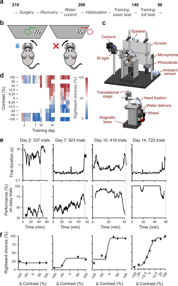
Standardized pipeline and apparatus, and training progression in the basic task.
(a) The pipeline for mouse surgeries and training. The number of animals at each stage of the pipeline is shown in bold. (b) Schematic of the task, showing the steering wheel and the visual stimulus moving to the center of the screen vs. the opposite direction, with resulting reward vs. timeout. (c) CAD model of the behavioral apparatus. Top: the entire apparatus, showing the back of the mouse. The screen is shown as transparent for illustration purposes. Bottom: side view of the detachable mouse holder, showing the steering wheel and water spout. A 3D rendered video of the CAD model can be found here. (d) Performance of an example mouse (KS014, from Lab 1) throughout training. Squares indicate choice performance for a given stimulus on a given day. Color indicates the percentage of right (red) and left (blue) choices. Empty squares indicate stimuli that were not presented. Negative contrasts denote stimuli on the left, positive contrasts denote stimuli on the right. (e) Example sessions from the same mouse. Vertical lines indicate when the mouse reached the session-ending criteria based on trial duration (top) and accuracy on high-contrast (>=50%) trials (bottom) averaged over a rolling window of 10 trials (Figure 1—figure supplement 1). (f) Psychometric curves for those sessions, showing the fraction of trials in which the stimulus on the right was chosen (rightward choices) as a function of stimulus position and contrast (difference between right and left, i.e. positive for right stimuli, negative for left stimuli). Circles show the mean and error bars show ±68% confidence intervals. The training history of this mouse can be explored at this interactive web page.

Task trial structure.
Trials began with an enforced quiescent period during which the wheel must be kept still for at least 200 ms, after which was the visual stimulus onset and an audio tone to indicate the start of the closed-loop period. The feedback period began when a response was given or 60 s had elapsed since stimulus onset. On correct trials a reward was given and the stimulus remained in the center of the screen for 1 s. On incorrect trials, there was a noise burst and a 2 s timeout before the next trial.
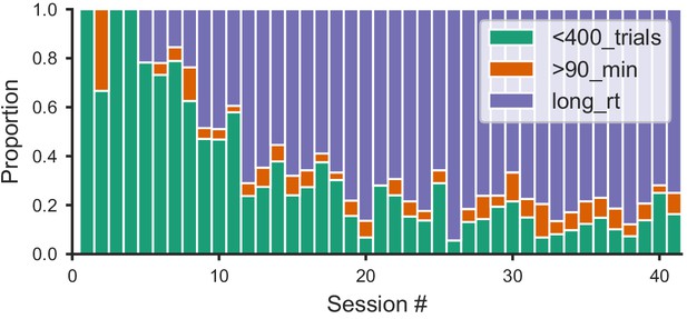
Distribution of within-session disengagement criteria.
The session ended if one of the three following criteria was met: either the mouse performed fewer than 400 trials in 45 min (not enough trials); or over 400 trials and the session length reached 90 min (session too long); or over 400 trials and its median reaction time (RT) over the last 20 trials was over 5x the median for the whole session (slow-down). Proportion of sessions that ended in each of the three criteria (colored in green; orange; blue, respectively) for all mice that learned the task.
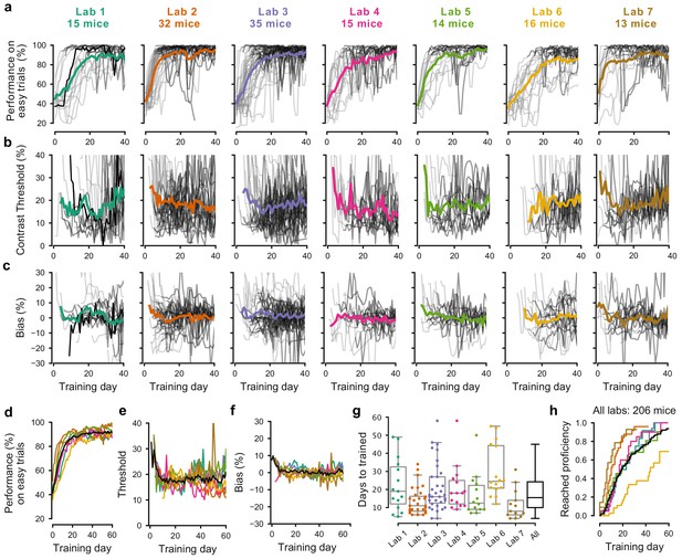
Learning rates differed across mice and laboratories.
(a) Performance for each mouse and laboratory throughout training. Performance was measured on easy trials (50% and 100% contrast). Each panel represents a different lab, and each thin curve represents a mouse. The transition from light gray to dark gray indicates when each mouse achieved proficiency in the basic task. Black, performance for example mouse in Figure 1. Thick colored lines show the lab average. Curves stop at day 40, when the automated training procedure suggests that mice be dropped from the study if they have not learned. (b) Same, for contrast threshold, calculated starting from the first session with a 12% contrast (i.e. first session with six or more different trial types), to ensure accurate psychometric curve fitting. Thick colored lines show the lab average from the moment there were three or more datapoints for a given training day. (c) Same, for choice bias. (d-f) Average performance, contrast threshold and choice bias of each laboratory across training days. Black curve denotes average across mice and laboratories (g) Training times for each mouse compared to the distribution across all laboratories (black). Boxplots show median and quartiles. (h) Cumulative proportion of mice to have reached proficiency as a function of training day (Kaplan-Meier estimate). Black curve denotes average across mice and laboratories. Data in (a-g) is for mice that reached proficiency (n = 140). Data in h is for all mice that started training (n = 206).
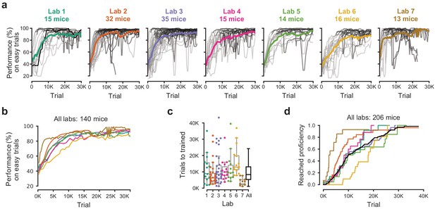
Learning rates measured by trial numbers.
(a) Performance curves for each mouse, for each laboratory. Performance was measured on easy trials (50% and 100% contrast). Each panel represents a lab, and each thin curve a mouse. The transition from light gray to dark gray indicates when each mouse achieved proficiency in the basic task. Black, performance for example mouse in Figure 1. Thick colored lines show the lab average. Curves stop at day 40, when the automated training procedure suggests that mice be dropped from the study if they have not learned. (b) Average performance curve of each laboratory across consecutive trials. (c) Number of trials to proficiency for each mouse compared to the distribution across all laboratories (black). Boxplots show median and quartiles. (d) Cumulative proportion of mice to have reached proficiency as a function of trials (Kaplan-Meier estimate). Black curve denotes average across mice and laboratories.
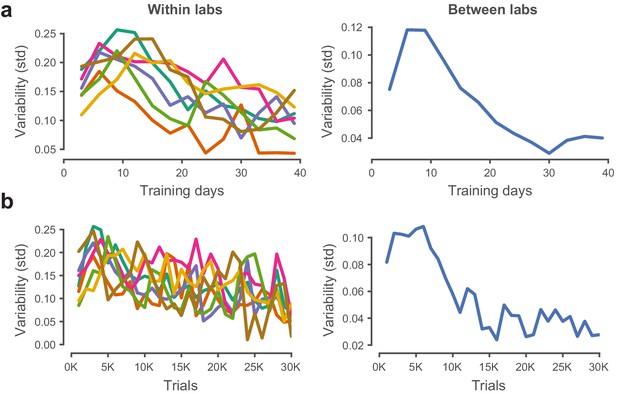
Performance variability within and across laboratories decreases with training.
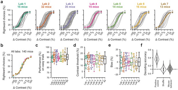
Performance in the basic task was indistinguishable across laboratories.
(a) Psychometric curves across mice and laboratories for the three sessions at which mice achieved proficiency on the basic task. Each curve represents a mouse (gray). Black curve represents the example mouse in Figure 1. Thick colored lines show the lab average. (b) Average psychometric curve for each laboratory. Circles show the mean and error bars ± 68% CI. (c) performance on easy trials (50% and 100% contrasts) for each mouse, plotted per lab and over all labs. Colored dots show individual mice and boxplots show the median and quartiles of the distribution. (d-e) Same, for contrast threshold and bias. (f) Performance of a Naive Bayes classifier trained to predict from which lab mice belonged, based on the measures in (c-e). We included the timezone of the laboratory as a positive control and generated a null-distribution by shuffling the lab labels. Dashed line represents chance-level classification performance. Violin plots: distribution of the 2000 random sub-samples of eight mice per laboratory. White dots: median. Thick lines: interquartile range.
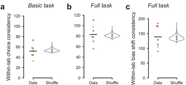
Mouse choices were no more consistent within labs than across labs.
To measure the similarity in choices across mice within a lab, we computed within-lab choice consistency. For each lab and each stimulus, we computed the variance across mice in the fraction of rightward choices. We then computed the inverse (consistency) and averaged the result across stimuli. (a) Within-lab choice consistency for the basic task (same data as in Figure 3) for each lab (dots) and averaged across labs (line). This averaged consistency was not significantly higher (p=0.73) than a null distribution generated by randomly shuffling lab assignments between mice and computing the average within-lab choice variability 10,000 times (violin plot). Therefore, choices were no more consistent within labs than across labs. (b) Same analysis, for the full task (same data as in Figure 4). Within-lab choice consistency on the full task was not higher than expected by chance, p=0.25. In this analysis we computed consistency separately for each stimulus and prior block before averaging across them. Choice consistency was higher on the full task than the basic task; this likely reflects both increased training on the task, and a stronger constraint on choice behavior through the full task’s block structure. (c) As in a, b, but measuring the within-lab consistency of ‘bias shift’ between the 20:80 and 80:20 blocks (as in Figure 4d,e). Within-lab consistency in bias shift was not higher than expected by chance (p=0.31).
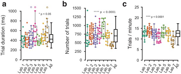
Behavioral metrics that were not explicitly harmonized showed small variation across labs.
(a) Average trial duration from stimulus onset to feedback, in the three sessions at which a mouse achieved proficiency in the basic task, shown for individual mice (dots) and as a distribution (box plots). (b) Same, for the average number of trials in each of the three sessions. (c) Same, for the number of trials per minute. Each dot represents a mouse, empty dots denote outliers outside the plotted y-axis range.
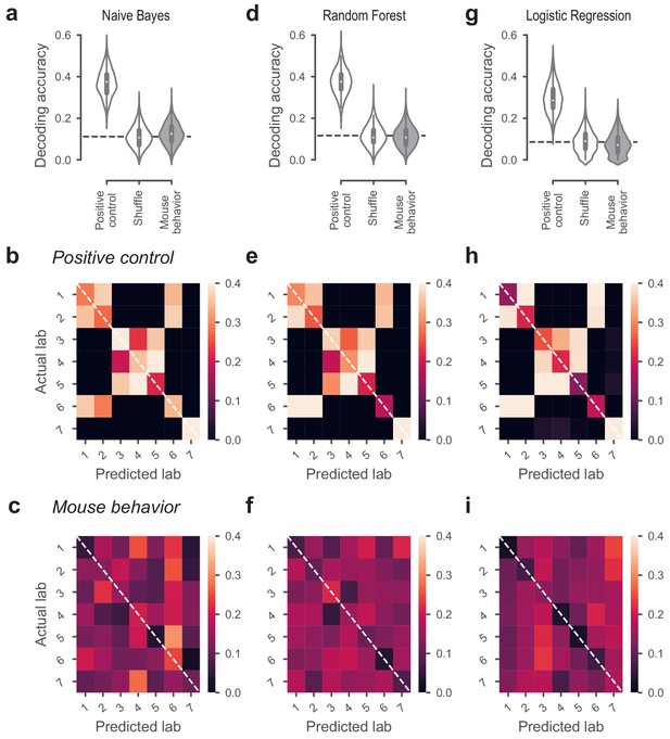
Classifiers could not predict lab membership from behavior.
(a) Classification performance of the Naive Bayes classifier that predicted lab membership based on behavioral metrics from Figure 3. In the positive control, the classifier had access to the time zone in which a mouse was trained. In the shuffle condition, the lab labels were randomly shuffled. (b) Confusion matrix for the positive control, showing the proportion of occurrences that a mouse from a given lab (y-axis) was classified to be in the predicted lab (x-axis). Labs in the same time zone from clear clusters, and Lab seven was always correctly predicted because it’s the only lab in its time zone. (c) Confusion matrix for the classifiers based on mouse behavior. The classifier was generally at chance and there was no particular structure to its mistakes. (d-f) Same, for the Random Forest classifier. (g–i) Same, for the Logistic Regression classifier.
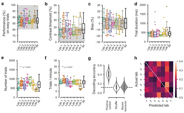
Comparable performance across institutions when using a reduced inclusion criterion (>=80% performance on easy trials).
(a) Performance on easy trials (50% and 100% contrasts) for each mouse, plotted over all labs (n = 150 mice). Colored dots show individual mice and boxplots show the median and quartiles of the distribution. (b–f) Same, for (b) contrast threshold, (c) bias, (d) trial duration and (e–f) trials completed per session. As it was the case with our standard inclusion criteria (Figure 3—figure supplement 2), there was a small but significant difference in the number of trials per session across laboratories. All other measured parameters were similar. (g) Performance of a Naive Bayes classifier trained to predict from which lab mice belonged, based on the measures in a-c. We included the timezone of the laboratory as a positive control and generated a null-distribution by shuffling the lab labels. Dashed line represents chance-level classification performance. Violin plots: distribution of the 2000 random sub-samples of 8 mice per laboratory. White dots: median. Thick lines: interquartile range. (h) Confusion matrix for the classifiers based on mouse behavior with reduced inclusion criteria. The classifier was at chance and there was no particular structure to its mistakes.
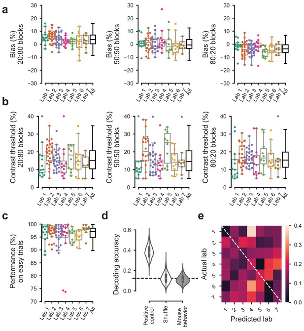
Behavior was indistinguishable across labs in the first 3 sessions of the full task.
For the first 3 sessions of performing the full task (triggered by achieving proficiency in the basic task, defined by a set of criteria, Figure 1—figure supplement 1d). (a) Bias for each block prior did not vary significantly over labs (Kruskal-Wallis test, 20:80 blocks; p=0.96, 50:50 block; p=0.96, 80:20 block; p=0.89). (b) The contrast thresholds also did not vary systematically over labs (Kruskal-Wallis test, 20:80 block; p=0.078, 50:50 block; p=0.12, 80:20 block; p=0.17). (c) Performance on 100% contrast trials neither (Kruskal-Wallis test, p=0.15). (d) The Naive Bayes classifier trained on the data in (a–c) did not perform above chance level when trying to predict the lab membership of mice. (e), Normalized confusion matrix for the classifier in (d).
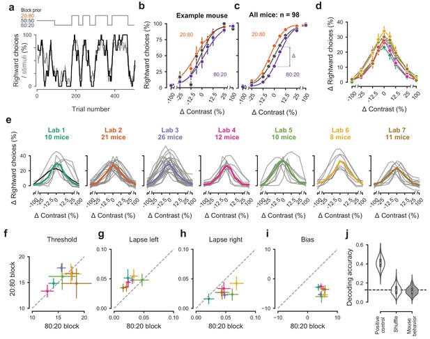
Mice successfully integrate priors into their decisions and task strategy.
(a) Block structure in an example session. Each session started with 90 trials of 50:50 prior probability, followed by alternating 20:80 and 80:20 blocks of varying length. Presented stimuli (gray, 10-trial running average) and the mouse’s choices (black, 10-trial running average) track the block structure. (b) Psychometric curves shift between blocks for the example mouse. (c) For each mouse that achieved proficiency on the full task (Figure 1—figure supplement 1d) and for each stimulus, we computed a ‘bias shift’ by reading out the difference in choice fraction between the 20:80 and 80:20 blocks (dashed lines). (d) Average shift in rightward choices between block types, as a function of contrast for each laboratory (colors as in 2 c, 3 c; error bars show mean ±68% CI). (e) Shift in rightward choices as a function of contrast, separately for each lab. Each line represents an individual mouse (gray), with the example mouse in black. Thick colored lines show the lab average. (f) Contrast threshold, (g) left lapses, (h) right lapses, and (i) bias separately for the 20:80 and 80:20 block types. Each lab is shown as mean +- s.e.m. (j) Classifier results as in 3 f, based on all data points in (f-i).
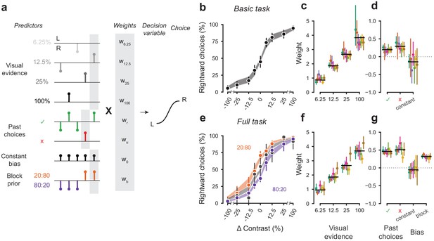
A probabilistic model reveals a common strategy across mice and laboratories.
(a) Schematic diagram of predictors included in the GLM. Each stimulus contrast (except for 0%) was included as a separate predictor. Past choices were included separately for rewarded and unrewarded trials. The block prior predictor was used only to model data obtained in the full task. (b) Psychometric curves from the example mouse across three sessions in the basic task. Shadow represents 95% confidence interval of the predicted choice fraction of the model. Points and error bars represent the mean and across-session confidence interval of the data. (c-d) Weights for GLM predictors across labs in the basic task, error bars represent the 95% confidence interval across mice. (e-g), as b-d but for the full task.
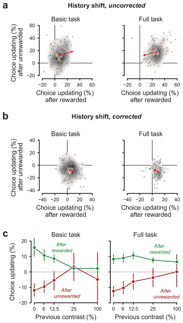
History-dependent choice updating.
(a) Representing each animal’s ‘history strategy’, defined as the bias shift in their psychometric function as a function of the choice made on the previous trial, separately for when this trial was rewarded or unrewarded. Each animal is shown as a dot, with lab-averages shown larger colored dots. Contours indicate a two-dimensional kernel density estimate across all animals. The red arrow shows the group average in the basic task at its origin, and in the full task at its end (replicated between the left and right panel). (b) as a, but with the strategy space corrected for slow fluctuations in decision bound (Lak et al., 2020a). When taking these slow state-changes into account, the majority of animals use a win-stay lose-switch strategy. (c) History-dependent choice updating, after removing the effect of slow fluctuations in decision bound, as a function of the previous trial’s reward and stimulus contrast. After rewarded trials, choice updating is largest when the visual stimulus was highly uncertain (i.e. had low contrast) but strongly diminished after more certain, rewarded trials. This is in line with predictions from Bayesian models, where an agent continually updates its beliefs about the upcoming stimuli with sensory evidence (Lak et al., 2020a; Mendonça et al., 2018). Appendices.
Parameters of the GLM model of choice across labs.
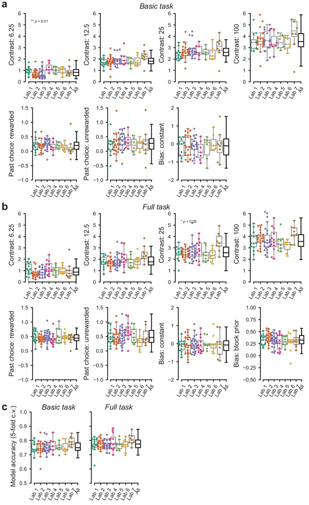
(a) Parameters of the GLM model for data obtained in the basic task. (b) Same, for the full task the additional panel shows the additional parameter, that is the bias shift in the two blocks. Each point represents the average accuracy for each mouse. (c) Cross validated accuracy of the GLM model across mice and laboratories. Predictions were considered accurate if the GLM predicted the actual choice with >50% chance.
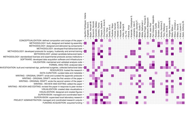
Contribution diagram.
The following diagram illustrates the contributions of each author, based on the CRediT taxonomy (Brand et al., 2015). For each type of contribution there are three levels indicated by color in the diagram: 'support’ (light), ‘equal’ (medium) and ‘lead’ (dark).
Tables
Standardization.
a, To facilitate reproducibility we standardized multiple aspects of the experiment. Some variables were kept strictly the same across mice, while others were kept within a range or simply recorded (see ‘Standardized’ column). b-c, The behavior training protocol was also standardized. Several task parameters adaptively changed within or across sessions contingent on various performance criteria being met, including number of trials completed, amount of water received and proportion of correct responses.
| A | ||||
|---|---|---|---|---|
| Category | Variable | Standardized | Standard | Recorded |
| Animal | Weight | Within a range | 18–30 g at headbar implant | Per session |
| Age | Within a range | 10–12 weeks at headbar implant | Per session | |
| Strain | Exactly | C57BL/6J | Once | |
| Sex | No | Both | Once | |
| Provider | Two options | Charles River (EU) Jax (US) | Once | |
| Training | Handling | One protocol | Protocol 2 | No |
| Hardware | Exactly | Protocol 3 | No | |
| Software | Exactly | Protocol 3 | Per session | |
| Fecal count | N/A | N/A | Per session | |
| Time of day | No | As constant as possible | Per session | |
| Housing | Enrichment | Minimum requirement | At least nesting and house | Once |
| Food | Within a range | Protein: 18–20%, Fat: 5–6.2% | Once | |
| Light cycle | Two options | 12 Hr inverted or non-inverted | Once | |
| Weekend water | Two options | Citric acid water or measured water | Per session | |
| Co housing status | No | Co-housing preferred, separate problem mice | Per change | |
| Surgery | Aseptic protocols | One protocol | Protocol 1 | No |
| Tools/Consumables | Required parts | Protocol 1 | No | |
| B | ||||
| Adaptive parameter | Initial value | |||
| Contrast set | [100, 50] | |||
| Reward volume | 3 μL | |||
| Wheel gain | 8 deg/mm | |||
| C | ||||
| Criterion | Outcome | |||
| >200 trials completed in previous session | Wheel gain decreased 4 deg/mm | |||
| >80% correct on each contrast | Contrast set = [100, 50, 25] | |||
| >80% correct on each contrast after above | Contrast set = [100, 50, 25, 12.5] | |||
| 200 trials after above | Contrast set = [100, 50, 25, 12.5, 6.25] | |||
| 200 trials after above | Contrast set = [100, 50, 25, 12.5, 6.25, 0] | |||
| 200 trials after above | Contrast set = [100, 25, 12.5, 6.25, 0] | |||
| 200 trials completed in previous session and reward volume > 1.5 μL | Decrease reward by 0.1 μL | |||
| Animal weight/25 > reward vol/1000 and reward volume < 3 μL | Next session increase reward by 0.1 μL | |||
| D | ||||
| Proficiency level | Outcome | |||
| ‘Basic task proficiency’ - Trained 1a/1b For each of the last three sessions: >200/400 trials completed, and >80%/90% correct on 100% contrast and all contrasts introduced and For the last three sessions combined: psychometric absolute bias < 16/10 and psychometric threshold < 19/20 and psychometric lapse rates < 0.2/0.1 For 1b only: median reaction time at 0% contrast < 2 s | Training in the basic task achieved: mouse is ready to proceed to training in the full task. In some mice, we continued training in the basic task to obtain even higher performance. (Guideline was to train mice for up to 40 days at Level 1, and drop mice from the study if they did not reach proficiency in this period). | |||
| ‘Full task proficiency’ For each of the last three sessions: >400 trials completed, and >90% correct on 100% contrast and For the last three sessions combined: all four lapse rates (left and right, 20:80 and 80:20 blocks)<0.1 and bias[80:20] - bias[20:80]>5 and median RT on 0% contrast < 2 s | Training in the full task achieved: mouse is ready for neural recordings. | |||


