Figures and data in Mathematical relationships between spinal motoneuron properties

Figures
Tables
Additional files

11 figures, 12 tables and 1 additional file

Figures

Figure 1

Download asset Open asset

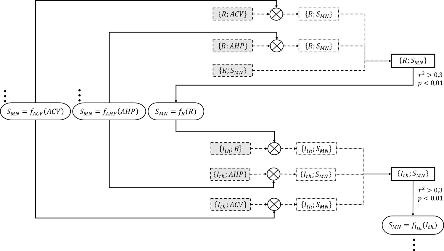
Detailed example for the process adopted to successively create the two final ${R; S_{M N}}$ and ${I_{t h}; S_{M N}}$ datasets (right-side thick-solid contour rectangular boxes).

These final datasets were obtained from respectively three and three normalized global datasets of experimental data obtained from the literature (dashed-contour grey-filled boxes) ${{R; A C V}, {R; A H P}, {R; S_{M N}}}$ and ${{I_{t h}; R}, {I_{t h}; A H P}, {I_{t h}; A C V}}$ . The ${R; A C V}$ and ${R; A H P}$ datasets were first transformed (⊗ symbol) into two intermediary ${R; S_{M N}}$ datasets (dotted-contour boxes) by converting the $A C V$ and $A H P$ values to equivalent $S_{M N}$ values with two ‘inverse’ $S_{M N} = f_{A C V} (A C V)$ and $S_{M N} = f_{A H P} (A H P)$ power relationships (oval boxes with triple dots), which had been previously obtained from two unshown steps that had yielded the final ${A C V; S_{M N}}$ and ${A H P; S_{M N}}$ datasets. The two intermediary ${R; S_{M N}}$ datasets were merged with the remaining global ${R; S_{M N}}$ dataset to yield the final ${R; S_{M N}}$ dataset, to which a power relationship of the form $R = k \cdot S_{M N}^{c}$ was fitted. If $r^{2} > 0.3$ and p<0.01, an ‘inverse’ power relationship $S_{M N} = f_{R} (R)$ (oval box) was further fitted to this final dataset. In a similar approach, the three normalized global datasets ${I_{t h}; R}, {I_{t h}; A H P}$ , and ${I_{t h}; A C V}$ were transformed with the three ‘inverse’ relationships into intermediary ${I_{t h}; S_{M N}}$ datasets, which were merged to yield the final ${I_{t h}; S_{M N}}$ dataset. An ‘inverse’ $S_{M N} = f_{I_{t h}} (I_{t h})$ power relationship was further derived to be used in the creation of the final ${C; S_{M N}}$ and ${τ; S_{M N}}$ datasets in the next taken steps.

Figure 2

Download asset Open asset

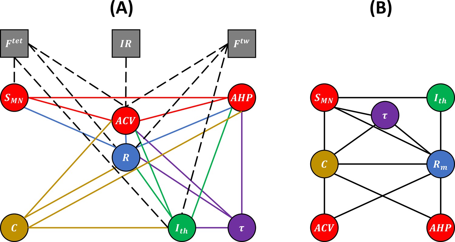
Experimental (A) and unknown (B) relations between motoneuron (MN) and muscle unit (mU) properties.

(A) Bubble diagram representing the pairs of MN and/or mU properties that could be investigated in this study from the results provided by the 40 studies identified in our web search. MN and mU properties are represented by circle and square bubbles, respectively. Relationships between MN properties are represented by coloured connecting lines; the colours red, blue, green, yellow, and purple are consistent with the order $A C V, A H P, R, I_{t h}, C, τ$ in which the pairs were investigated (see Table 3 for mathematical relationships). Relationships between one MN and one mU property are represented by black dashed lines. (B) Bubble diagram representing the mathematical relationships proposed in this study between pairs of MN properties for which no concurrent experimental data has been measured to date.

Figure 3

Download asset Open asset

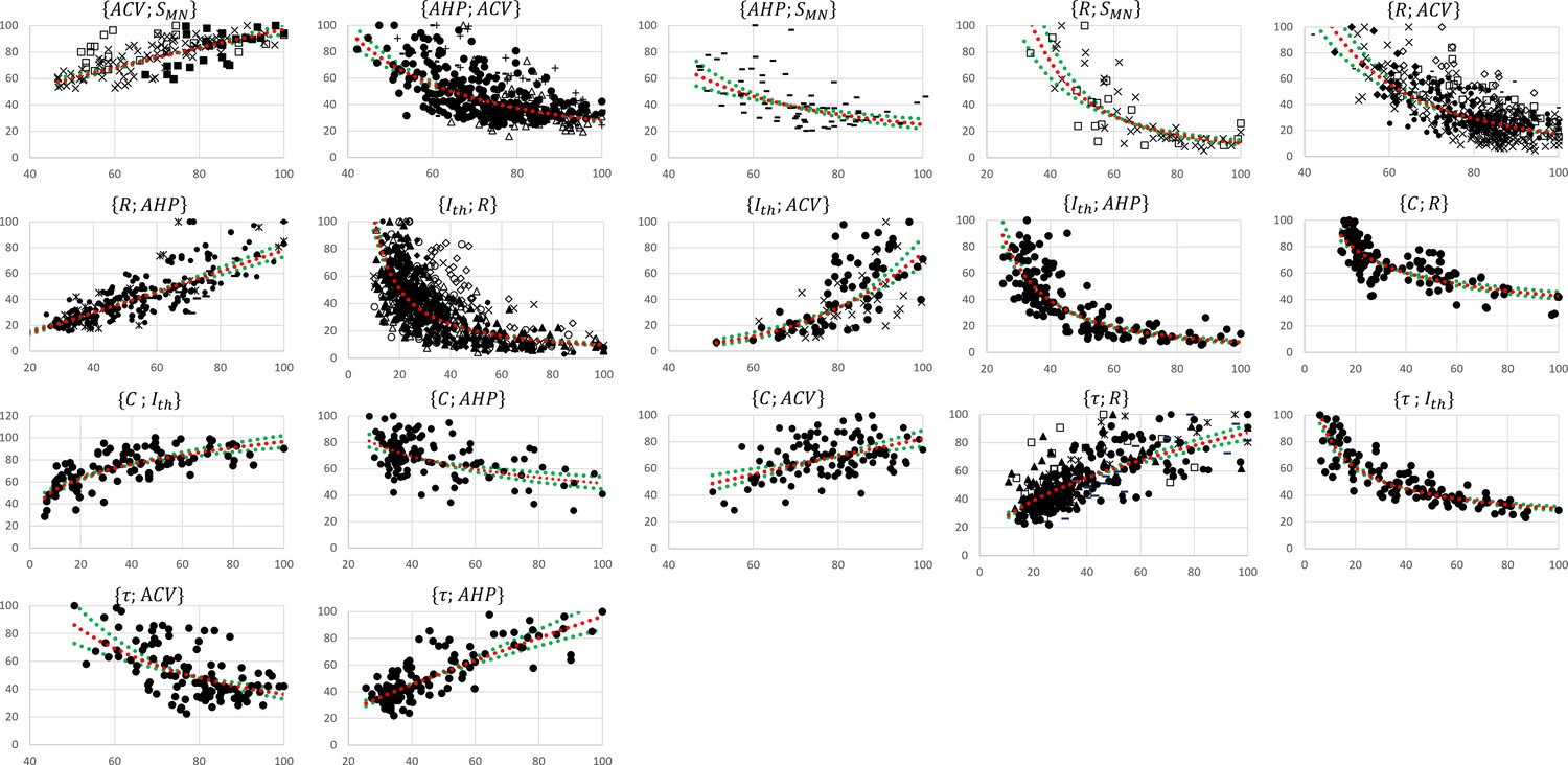
Normalized global datasets.

These were obtained from the 19 studies reporting cat data that measured and investigated the 17 pairs of motoneuron (MN) properties reported in Figure 2A. For each ${A; B}$ pair, the property $A$ is read on the y-axis and $B$ on the x-axis. For information, power trendlines $A = k \cdot B^{a}$ (red dotted curves) are fitted to the data of each dataset and reported in Table 3. The 95% confidence interval of the regression is also displayed for each dataset (green dotted lines). The studies are identified with the following symbols: • (Gustafsson, 1979; Gustafsson and Pinter, 1984a; Gustafsson and Pinter, 1984b), ○ (Munson et al., 1986), ▲ (Zengel et al., 1985), ∆ (Foehring et al., 1987), ■ (Cullheim, 1978), □ (Burke, 1968; Burke and ten Bruggencate, 1971; Burke et al., 1982), ◆(Krawitz et al., 2001), ◇ (Fleshman et al., 1981), + (Eccles et al., 1958b), ☓ (Kernell, 1966; Kernell and Zwaagstra, 1981; Kernell and Monster, 1981), - (Zwaagstra and Kernell, 1980), — (Sasaki, 1991), ✶ (Pinter and Vanden Noven, 1989). The axes are given in % of the maximum retrieved values in the studies consistently with ‘Methods’ section.

Figure 3—source data 1 All the cat datasets presented in Figure 3.: https://cdn.elifesciences.org/articles/76489/elife-76489-fig3-data1-v2.xlsx
Download elife-76489-fig3-data1-v2.xlsx

Figure 4

Download asset Open asset

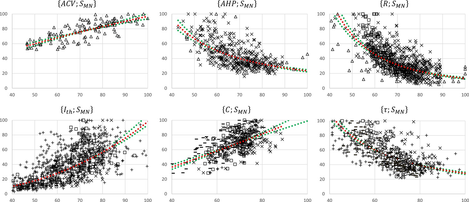
Normalized motoneuron (MN) size-related final datasets.

These were obtained from the 19 studies reporting cat data that concurrently measured at least two of the morphometric and electrophysiological properties listed in Table 1. For each ${A; S_{M N}}$ pair, the property $A$ is read on the y-axis and $S_{M N}$ on the x-axis. The power trendlines $A = k_{c} \cdot S_{M N}^{c}$ (red dotted curves) are fitted to each dataset and are reported in Table 3. The 95% confidence interval of the regression is also displayed for each dataset (green dotted lines). For each ${A; S_{M N}}$ plot, the constitutive sub-datasets ${A; S_{M N}}$ that were obtained from different global ${A; B}$ datasets are specified with the following symbols identifying the property $B$ : $S_{M N} \leftrightarrow Δ$ , $A C V \leftrightarrow \times$ , $A H P \leftrightarrow$ □, $R \leftrightarrow +$ , and $I_{t h} \leftrightarrow -$ .

Figure 5

Download asset Open asset

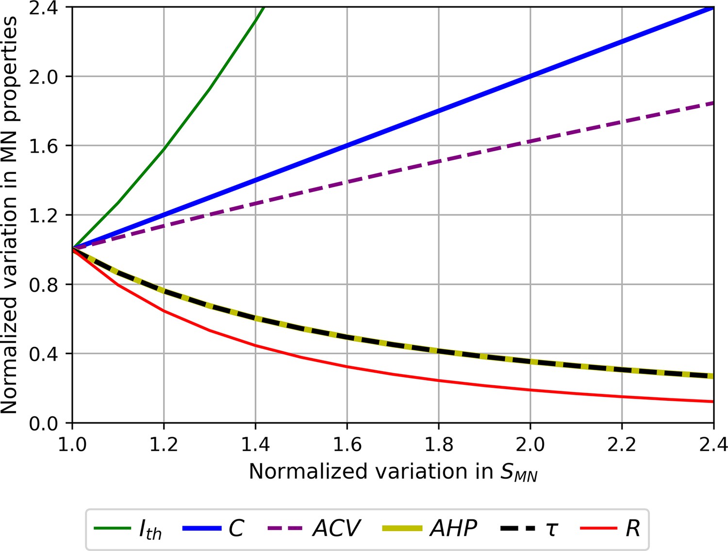
Normalized size-dependent behaviour of the motoneuron (MN) properties $A C V, A H P, R, I_{t h}, C$ , and $τ$ .

For displaying purposes, the MN properties are plotted in arbitrary units as power functions (intercept $k = 1$ ) of $S_{M N}$ : $A = S_{M N}^{c}$ according to Table 3. The larger the MN size, the larger $A C V$ , $C$ , and $I_{t h}$ in the order of increasing slopes, and the lower $A H P$ , $τ$ and $R$ in the order of increasing slopes.

Figure 6

Download asset Open asset

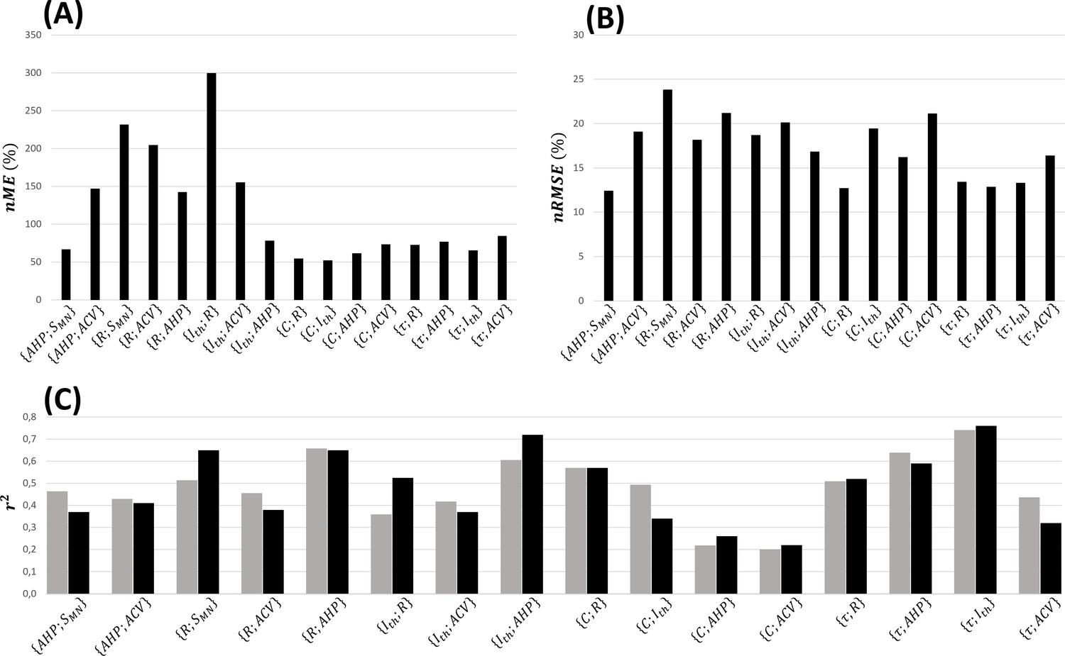
Fivefold cross-validation of the normalized mathematical relationships.

Here are reported for each dataset the average values across the five permutations of (A) the normalized maximum error ( $n M E$ ), (B) the normalized root mean square error ( $n R M S E$ ), and (C) coefficient of determination ( $r_{p r e d}^{2}$ , grey bars), which is compared with the coefficient of determination ( $r_{e x p}^{2}$ , black bars) of the power trendline fitted to the log–log transformation of global experimental datasets directly.

Figure 7

Download asset Open asset

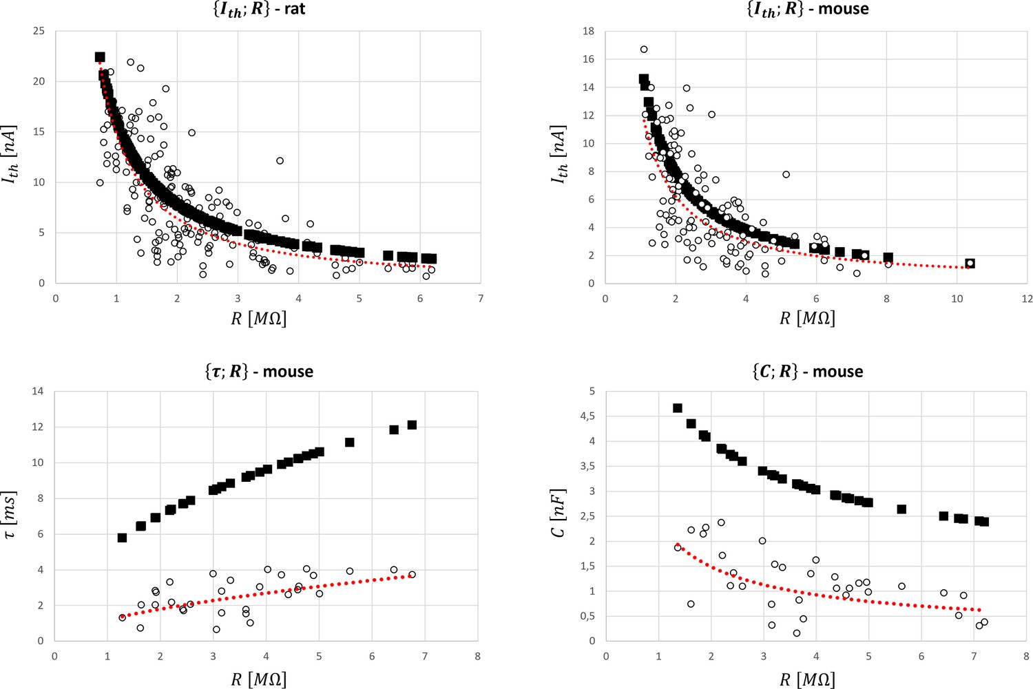
Global datasets for rat and mouse species and predictions of the motoneuron (MN) properties with the cat mathematical relationships (Table 4).

They were obtained from the five studies reporting data on rats and the four studies presenting data on mice reported in Appendix 1—table 5 that measured the ${I_{t h}; R}$ , ${τ; R}$ , and ${C; R}$ pairs of MN electrophysiological properties. $I_{t h}, R, τ, C$ are given in nA, MΩ, ms, and nF, respectively. The experimental data (○ symbol) is fitted with a power trendline (red dotted curve) and compared to the predicted quantities obtained with the scaled cat relationships in Table 4 (■ symbol).

Figure 7—source data 1 Datasets used in the rat plot.: https://cdn.elifesciences.org/articles/76489/elife-76489-fig7-data1-v2.xlsx
Download elife-76489-fig7-data1-v2.xlsx
Figure 7—source data 2 Datasets used in the mouse plots.: https://cdn.elifesciences.org/articles/76489/elife-76489-fig7-data2-v2.xlsx
Download elife-76489-fig7-data2-v2.xlsx

Appendix 1—figure 1

Download asset Open asset

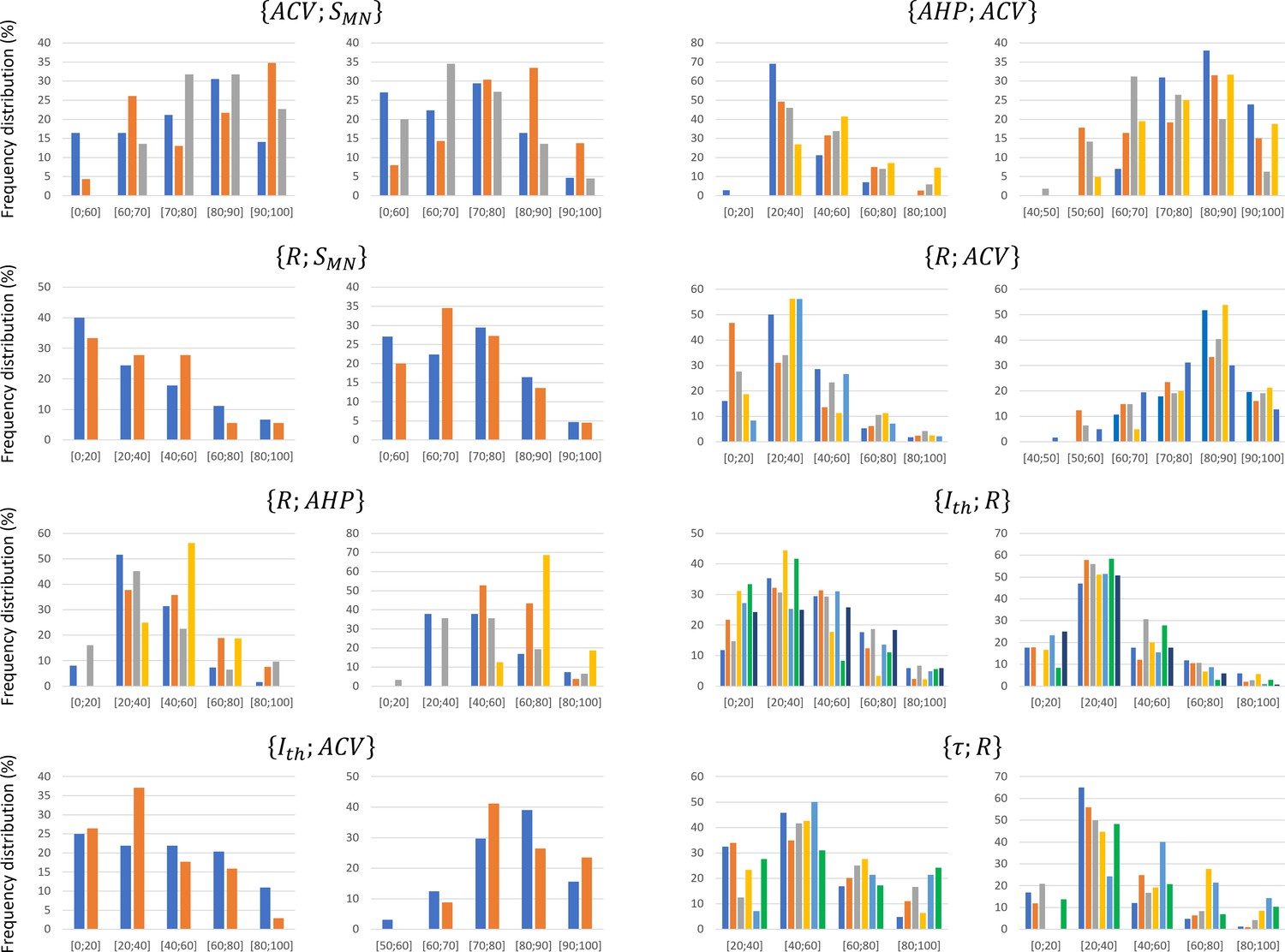
Density histograms of the data distributions reported in the experimental studies included in the global datasets.

Depending on the typical range over which each property spans, the distributions are divided in steps of 10 or 20%. The frequency distribution is provided in percentage of the total number of reported data points in a study. Different studies are displayed with different colours in each graph. For each dataset ${A; B}$ , the frequency distributions of property $A$ and $B$ are provided in the left and right plot, respectively.

Appendix 1—figure 2

Download asset Open asset

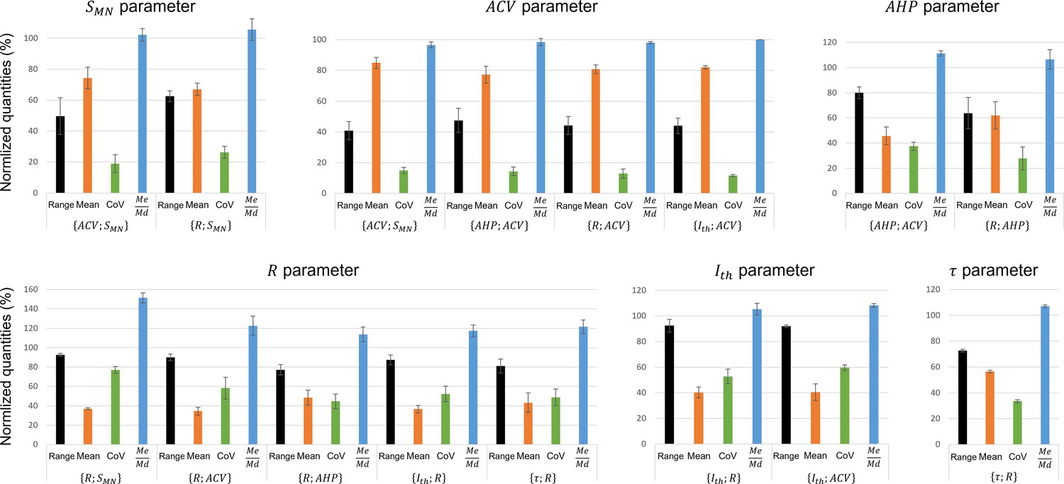
Assessment of data variability between the experimental studies that constitute the eight global datasets that include at least two experimental studies.

For each experimental study included in the global dataset ${A; B}$ , the range, mean, coefficient of variation $(C o V = \frac{s t a n d a r d d e v i a t i o n}{M e a n})$ , and the ratio $\frac{M e}{M d} = \frac{M e a n}{M e d i a n}$ of the experimental $A$ values measured in this study were computed. Then, the average (bars) and standard deviation (error bars) across experimental studies of these four metrics (range, mean, CoV, $\frac{M e}{M d}$ ) were calculated for each global dataset independently. For example, the first bar in the ‘ $S_{M N}$ parameter’ plot represents the average across three studies (Kernell and Zwaagstra, 1981; Cullheim, 1978; Burke et al., 1982) of the range of $S_{M N}$ values reported in these studies, for the global dataset ${A C V; S_{M N}}$ . The computed standard deviations (error bars) express for each global dataset the inter-study variability of (1) the length of the identified bandwidth of the motoneuron (MN) pool (range metric), (2) the spread of values around the mean (CoV metric), (3) the skewness of the distributions, and (4) whether the distributions from different studies are centred (mean metric). A global dataset ${A; B}$ reporting narrow error bars for parameter $A$ for the four metrics infers that the experimental studies constituting this dataset measured similar distributions of property $A$ .

Appendix 1—figure 3

Download asset Open asset

Distribution of the size of the experimental datasets constituting the global datasets for assessment of the variability in the input data.

The histogram is divided between global datasets (half vertical lines), grouped as final size-dependent datasets (full vertical lines). For each global dataset, the total number of data points is reported (label: ‘N’), while the size of the constitutive experimental studies is reported in decreasing order.

Appendix 1—figure 4

Download asset Open asset

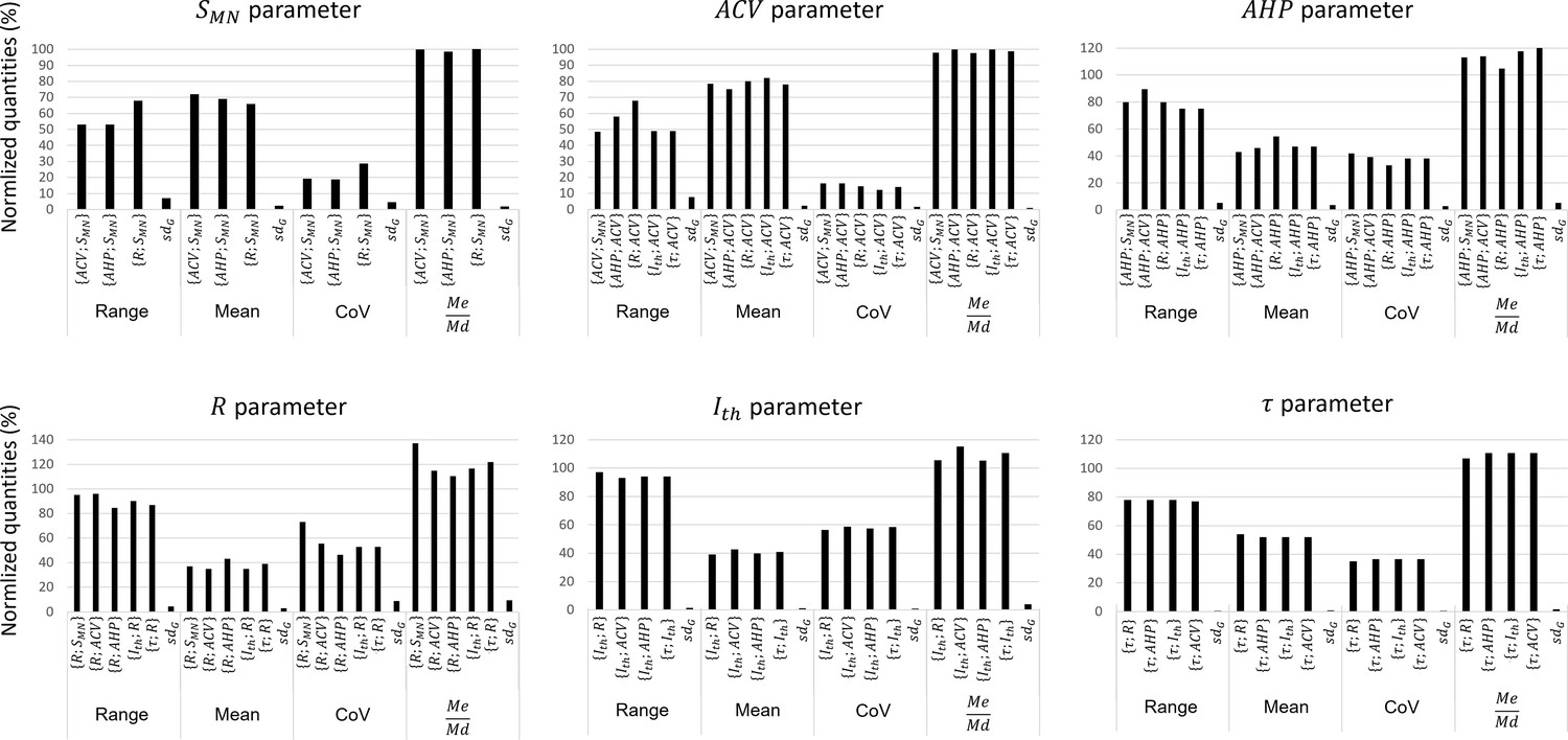
Assessment of data variability between the global datasets.

This figure compares the distributions of the $S_{M N}, A C V, A H P, R, I_{t h}$ , and $τ$ properties between the normalized global datasets built in this study. For each property, the range, mean, coefficient of variation $(o V = \frac{s t a n d a r d d e v i a t i o n}{M e a n})$ , and the ratio $\frac{M e}{M d} = \frac{M e a n}{M e d i a n}$ of its distribution in a global dataset is compared to the other global datasets it appears in. For each property, the standard deviation $s d_{G}$ between global datasets of these four metrics is computed. A low $s d_{G}$ value reflects the low variability of the property distribution between global datasets.

Tables

Table 1

The motoneuron (MN) and muscle unit (mU) properties investigated in this study with their notations and SI base units.

$S_{M N}$ is the size of the MN. As reproduced in Table 2, the MN size $S_{M N}$ is adequately described by measures of the MN surface area $S_{n e u r o n}$ and the soma diameter $D_{s o m a}$ . $R$ and $R_{m}$ define the MN-specific electrical resistance properties of the MN and set the value of the MN-specific current threshold $I_{t h}$ (Binder et al., 1996; Powers and Binder, 2001; Heckman and Enoka, 2012). C and $C_{m}$ (constant among the MN pool) define the capacitance properties of the MN and contribute to the definition of the MN membrane time constant τ (Gustafsson and Pinter, 1984a; Zengel et al., 1985). $∆ V_{t h}$ is the amplitude of the membrane voltage depolarization threshold relative to resting state required to elicit an action potential. $I_{t h}$ is the corresponding electrical current causing a membrane depolarization of $∆ V_{t h}$ . AHP duration is defined in most studies as the duration between the action potential onset and the time at which the MN membrane potential meets the resting state after being hyperpolarized. ACV is the axonal conduction velocity of the elicited action potentials on the MN membrane. $S_{m U}$ is the size of the mU. As indicated in Table 2, the mU size $S_{m U}$ is adequately described by measures of (1) the sum of the cross-sectional areas (CSAs) of the fibres composing the mU $C S A^{t o t}$ , (2) the mean fibre CSA $C S A^{m e a n}$ , (3) the innervation ratio IR, that is, the number of innervated fibres constituting the mU, and (4) the mU tetanic force $F^{t e t}$ . $F^{t w}$ is the MU twitch force.

	Properties	Notation	Unit
MN properties	Size: Neuron surface area Soma diameter	$S_{M N}$ $S_{n e u r o n}$ $D_{s o m a}$	$[m^{2}]$ $[m]$
	Resistance	$R$	$[Ω]$
	Specific resistance per unit area	$R_{m}$	$[Ω \cdot m^{2}]$
	Capacitance	$C$	$[F]$
	Specific capacitance per unit area	$C_{m}$	$[F \cdot m^{- 2}]$
	Time constant	$τ$	$[s]$
	Rheobase (current recruitment threshold)	$I_{t h}$	$[A]$
	Voltage threshold	$∆ V_{t h}$	$[V]$
	Afterhyperpolarization duration	$A H P$	$[s]$
	Axonal conduction velocity	$A C V$	$[m \cdot s^{- 1}]$
mU properties	Size:	$S_{m U}$
	Total fibre cross-sectional area	$C S A^{t o t}$	$[m^{2}]$
	Mean fibre cross-sectional area	$C S A^{m e a n}$	$[m^{2}]$
	Innervation ratio	$I R$	$[]$
	Tetanic force	$F^{t e t}$	$[N]$
	Twitch force	$F^{t w}$	$[N]$

Table 2

Measurable indices of motoneuron (MN) and muscle unit (mU) sizes in mammals.

$S_{M N}$ and $S_{m U}$ are conceptual parameters which are adequately described by the measurable and linearly inter-related quantities reported in this table.

MN size (S_MN)	mU size (S_mU)
$S_{n e u r o n}$	$F^{t e t}$
$D_{s o m a}$	$I R$
	$C S A^{m e a n}$
	$C S A^{t o t}$

Table 3

Fitted experimental data of pairs of motoneuron (MN) properties and subsequent normalized final size-related relationships.

For information, the $r^{2}$ , p-value, and the equation $A = k_{a} ∙ B^{a}$ are reported for each fitted global dataset. The normalized MN-size dependent relationships $A = k_{c} ∙ S_{M N}^{c}$ are mathematically derived from the transformation of the global datasets and from the power trendline fitting of the final datasets (N data points) as described in ‘Methods’. The minimum and maximum values of $k_{a}, k_{c}, a$ , and $c$ defining the 95% confidence interval of the regression are also reported in parenthesis for each global and final dataset. The $r^{2}$ values reported in this table are consistent with the $r^{2}$ values obtained when directly fitting the normalized experimental datasets with power regressions (see Appendix 1—table 1).

MN property	$A = k_{a} \cdot B^{a}$ (normalized global datasets)						$A = k_{c} \cdot S_{M N}^{c}$ (final MN-size dependent datasets)
$A$	Relationship	$k_{a}$	$a$	$r^{2}$	p-value	Reference studies	$k_{c}$	$c$	$r^{2}$	p-value	$N$ points
$A C V$	$A C V = k_{a} ∙ S_{M N}^{a}$	4.0 (2.5; 6.4)	0.7 (0.6; 0.8)	0.58	< 10^-5	Cullheim, 1978; Kernell and Zwaagstra, 1981; Burke et al., 1982	4.0 (2.5; 6.4)	0.7 (0.6; 0.8)	0.58	< 10^-5	109
$A H P$	$A H P = k_{a} ∙ S_{M N}^{a}$	6.1 · 10³ (1.2 · 10³; 3.2 · 10⁴)	−1.2 (−1.6; −0.8)	0.34	< 10^-5	Zwaagstra and Kernell, 1980	2.5 · 10⁴ (1.2 · 10⁴; 5.0 · 10⁴)	−1.5 (−1.7; −1.3)	0.41	< 10^-5	492
$A H P$	$A H P = k_{a} ∙ {A C V}^{a}$	1.5 · 10⁴ (7.4 · 10³; 2.9 · 10⁴)	−1.4 (−1.5; −1.2)	0.41	< 10^-5	Eccles et al., 1958a; Zwaagstra and Kernell, 1980; Gustafsson and Pinter, 1984b; Foehring et al., 1987	2.5 · 10⁴ (1.2 · 10⁴; 5.0 · 10⁴)	−1.5 (−1.7; −1.3)	0.41	< 10^-5	492
$R$	$R = k_{a} ∙ S_{M N}^{a}$	1.5 · 10⁵ (2.7 · 10⁴; 7.9 · 10⁵)	−2.1 (−2.5; −1.7)	0.61	< 10^-5	Kernell and Zwaagstra, 1981; Burke et al., 1982	9.6 · 10⁵ (4.1 · 10⁵; 2.3 · 10⁶)	−2.4 (−2.6; −2.2)	0.37	< 10^-5	745
	$R = k_{a} ∙ A C V^{a}$	6.3 · 10⁵ (1.9 · 10⁵; 2.1 · 10⁶)	−2.3 (−2.6; −2.0)	0.38	< 10^-5	Kernell, 1966; Burke, 1968; Barrett and Crill, 1974; Kernell and Zwaagstra, 1981; Fleshman et al., 1981; Gustafsson and Pinter, 1984b; Sasaki, 1991
	$R = k_{a} ∙ A H P^{a}$	6.2 · 10⁻¹ (4.1 · 10⁻¹; 9.2 · 10⁻¹)	1.1 (0.9; 1.2)	0.65	< 10^-5	Gustafsson, 1979; Gustafsson and Pinter, 1984b; Foehring et al., 1987; Pinter and Vanden Noven, 1989; Sasaki, 1991
$I_{t h}$	$I_{t h} = k_{a} ∙ R^{a}$	1.1 · 10³ (0.8 · 10³; 1.3 · 10³)	−1.0 (−1.1; −0.9)	0.37	< 10^-5	Kernell, 1966; Fleshman et al., 1981; Gustafsson and Pinter, 1984a; Zengel et al., 1985; Munson et al., 1986; Foehring et al., 1987; Krawitz et al., 2001	9.0 · 10⁻⁴ (4.7 · 10⁻⁴; 1.7 · 10⁻³)	2.5 (2.4; 2.7)	0.37	< 10^-5	722
	$I_{t h} = k_{a} ∙ A C V^{a}$	3.2 · 10⁻⁶ (1.3 · 10⁻⁷; 8.2 · 10⁻⁵)	3.7 (3.0; 4.4)	0.37	< 10^-5	Kernell and Monster, 1981; Gustafsson and Pinter, 1984a
	$I_{t h} = k_{a} ∙ A H P^{a}$	2.5 · 10⁴ (1.3 · 10⁴; 4.8· 10⁴)	−1.7 (−1.9; −1.6)	0.60	< 10^-5	Gustafsson and Pinter, 1984a
$C$	$C = k_{a} ∙ R^{a}$	2.4 · 10² (2.0 · 10²; 3.9 · 10²)	−0.4 (−0.4; −0.3)	0.57	< 10^-5	Gustafsson and Pinter, 1984b	1.2 (0.7; 2.0)	1.0 (0.9; 1.2)	0.28	< 10^-5	444
	$C = k_{a} ∙ I_{t h}^{a}$	2.9 · 10¹ (2.4 · 10¹; 3.5 · 10¹)	0.3 (0.2; 0.3)	0.51	< 10^-5	Gustafsson and Pinter, 1984a
	$C = k_{a} ∙ A H P^{a}$	2.8 · 10² (1.8 · 10²; 4.4 · 10²)	−0.4 (−0.5; −0.3)	0.24	< 10^-5	Gustafsson and Pinter, 1984b
	$C = k_{a} ∙ A C V^{a}$	2.5 (0.7; 8.4)	0.8 (0.5; 1.0)	0.17	< 10^-5	Gustafsson and Pinter, 1984b
$τ$	$τ = k_{a} ∙ R^{a}$	8.7 (7.2; 10.6)	0.5 (0.4; 0.6)	0.52	< 10^-5	Burke and ten Bruggencate, 1971; Barrett and Crill, 1974; Gustafsson, 1979; Gustafsson and Pinter, 1984b; Zengel et al., 1985; Pinter and Vanden Noven, 1989; Sasaki, 1991	2.6 · 10⁴ (1.5 · 10⁴; 4.5 · 10⁴)	−1.5 (−1.6; −1.4)	0.46	< 10^-5	649
	$τ = k_{a} ∙ A H P^{a}$	2.2 (1.3; 3.5)	0.8 (0.7; 1.0)	0.63	< 10^-5	Gustafsson and Pinter, 1984b
	$τ = k_{a} ∙ I_{t h}^{a}$	2.3 · 10² (1.9 · 10²; 2.7 · 10²)	−0.4 (−0.5; −0.3)	0.72	< 10^-5	Gustafsson and Pinter, 1984a
	$τ = k_{a} ∙ A C V^{a}$	1.2 · 10⁴ (2.2 · 10³; 6.6 · 10⁴)	−1.3 (−1.7; −0.9)	0.30	< 10^-5	Gustafsson and Pinter, 1984b

Table 4

Mathematical empirical cat relationships between the motoneuron (MN) properties $S_{n e u r o n}, D_{s o m a}, R, R_{m}, C, τ, I_{t h},$ $A H P$ , and $A C V$ .

Each column provides the relationships between one and the eight other MN properties. If one property is known, the complete MN profile can be reconstructed by using the pertinent line in this table. All constants and properties are provided in SI base units (metres, seconds, ohms, farads, and amperes). The relationships involving $R_{m}$ were obtained from theoretical relationships involved in Rall’s cable theory (see ‘Discussion’).

	$S_{n e u r o n} [m^{2}]$	$D_{s o m a} [m]$	$R [Ω]$	$R_{m} [Ω \cdot m^{2}]$	$C [F]$	$τ [s]$	$I_{t h} [A]$	$A H P [s]$	$A C V [m \cdot s^{- 1}]$
$S_{n e u r o n} [m^{2}]$		$D_{s o m a} = 1.8 \cdot 10^{2} \cdot S_{n e u r o n}$	$R = \frac{1.7 \cdot 10^{- 10}}{S_{n e u r o n}^{2.43}}$	$R_{m} = \frac{1.0 \cdot 10^{- 10}}{S_{n e u r o n}^{1.43}}$	$C = 1.3 \cdot 10^{- 2} \cdot S_{n e u r o n}$	$τ = \frac{1.0 \cdot 10^{- 12}}{S_{n e u r o n}^{1.48}}$	$I_{t h} = 3.8 \cdot 10^{8} \cdot S_{n e u r o n}^{2.52}$	$A H P = \frac{1.0 \cdot 10^{- 11}}{S_{n e u r o n}^{1.51}}$	$A C V = 3.0 \cdot 10^{6} \cdot S_{n e u r o n}^{0.69}$
$D_{s o m a} [m]$	$S_{n e u r o n} = 5.5 \cdot 10^{- 3} \cdot D_{s o m a}$		$R = \frac{5.1 \cdot 10^{- 5}}{D_{s o m a}^{2.43}}$	$R_{m} = \frac{1.7 \cdot 10^{- 7}}{D_{s o m a}^{1.43}}$	$C = 7.9 \cdot 10^{- 5} \cdot D_{s o m a}$	$τ = \frac{2.3 \cdot 10^{- 9}}{D_{s o m a}^{1.48}}$	$I_{t h} = 7.8 \cdot 10^{2} \cdot D_{s o m a}^{2.52}$	$A H P = \frac{2.7 \cdot 10^{- 8}}{D_{s o m a}^{1.51}}$	$A C V = 8.1 \cdot 10^{4} \cdot D_{s o m a}^{0.69}$
$R [Ω]$	$S_{n e u r o n} = \frac{9.5 \cdot 10^{- 5}}{R^{0.41}}$	$D_{s o m a} = \frac{1.7 \cdot 10^{- 2}}{R^{0.41}}$		$R_{m} = 5.7 \cdot 10^{- 5} \cdot R^{0.59}$	$C = \frac{1.5 \cdot 10^{- 6}}{R^{0.40}}$	$τ = 9.6 \cdot 10^{- 7} \cdot R^{0.61}$	$I_{t h} = \frac{2.7 \cdot 10^{- 2}}{R^{1.04}}$	$A H P = 1.3 \cdot 10^{- 5} \cdot R^{0.62}$	$A C V = \frac{4.9 \cdot 10^{3}}{R^{0.29}}$
$R_{m} [Ω \cdot m^{2}]$	$S_{n e u r o n} = \frac{1.5 \cdot 10^{- 7}}{R_{m}^{0.70}}$	$D_{s o m a} = \frac{2.6 \cdot 10^{- 5}}{R_{m}^{0.70}}$	$R = 6.8 \cdot 10^{6} \cdot R_{m}^{1.70}$		$C = \frac{1.8 \cdot 10^{- 9}}{R_{m}^{0.69}}$	$τ = 1.4 \cdot 10^{- 2} \cdot R_{m}^{1.04}$	$I_{t h} = \frac{2.2 \cdot 10^{- 9}}{R_{m}^{1.76}}$	$A H P = 2.2 \cdot 10^{- 1} \cdot R_{m}^{1.06}$	$A C V = \frac{5.4 \cdot 10^{1}}{R_{m}^{0.48}}$
$C [F]$	$S_{n e u r o n} = 1.2 \cdot 10^{2} \cdot C$	$D_{s o m a} = 2.1 \cdot 10^{4} \cdot C$	$R = \frac{1.5 \cdot 10^{- 15}}{C^{2.48}}$	$R_{m} = \frac{1.7 \cdot 10^{- 13}}{C^{1.46}}$		$τ = \frac{8.6 \cdot 10^{- 16}}{C^{1.51}}$	$I_{t h} = 6.5 \cdot 10^{13} \cdot C^{2.57}$	$A H P = \frac{7.7 \cdot 10^{- 15}}{C^{1.54}}$	$A C V = 8.2 \cdot 10^{7} \cdot C^{0.71}$
$τ [s]$	$S_{n e u r o n} = \frac{8.4 \cdot 10^{- 9}}{τ^{0.67}}$	$D_{s o m a} = \frac{1.5 \cdot 10^{- 6}}{τ^{0.67}}$	$R = 7.1 \cdot 10^{9} \cdot τ^{1.64}$	$R_{m} = 3.6 \cdot 10^{1} \cdot τ^{0.96}$	$C = \frac{1.6 \cdot 10^{- 10}}{τ^{0.66}}$		$I_{t h} = \frac{1.6 \cdot 10^{- 12}}{τ^{1.70}}$	$A H P = 1.7 \cdot 10^{1} \cdot τ^{1.02}$	$A C V = \frac{7.5}{τ^{0.47}}$
$I_{t h} [A]$	$S_{n e u r o n} = 4.0 \cdot 10^{- 4} \cdot I_{t h}^{0.40}$	$D_{s o m a} = 7.1 \cdot 10^{- 2} \cdot I_{t h}^{0.40}$	$R = \frac{3.1 \cdot 10^{- 2}}{I_{t h}^{0.96}}$	$R_{m} = \frac{7.4 \cdot 10^{- 6}}{I_{t h}^{0.57}}$	$C = 5.9 \cdot 10^{- 6} \cdot I_{t h}^{0.39}$	$τ = \frac{1.2 \cdot 10^{- 7}}{I_{t h}^{0.59}}$		$A H P = \frac{1.5 \cdot 10^{- 6}}{I_{t h}^{0.60}}$	$A C V = 1.3 \cdot 10^{4} \cdot I_{t h}^{0.27}$
$A H P [s]$	$S_{n e u r o n} = \frac{5.5 \cdot 10^{- 8}}{A H P^{0.66}}$	$D_{s o m a} = \frac{9.8 \cdot 10^{- 6}}{A H P^{0.66}}$	$R = 7.5 \cdot 10^{7} \cdot A H P^{1.61}$	$R_{m} = 2.5 \cdot A H P^{0.95}$	$C = \frac{9.7 \cdot 10^{- 10}}{A H P^{0.65}}$	$τ = 6.2 \cdot 10^{- 2} \cdot A H P^{0.98}$	$I_{t h} = \frac{1.8 \cdot 10^{- 10}}{A H P^{1.67}}$		$A C V = \frac{2.7 \cdot 10^{1}}{A H P^{0.46}}$
$A C V [m \cdot s^{- 1}]$	$S_{n e u r o n} = 4.6 \cdot 10^{- 10} \cdot A C V^{1.44}$	$D_{s o m a} = 8.3 \cdot 10^{- 8} \cdot A C V^{1.44}$	$R = \frac{8.3 \cdot 10^{12}}{A C V^{3.50}}$	$R_{m} = \frac{2.3 \cdot 10^{3}}{A C V^{2.06}}$	$C = 9.0 \cdot 10^{- 12} \cdot A C V^{1.41}$	$τ = \frac{7.4 \cdot 10^{1}}{A C V^{2.14}}$	$I_{t h} = 1.1 \cdot 10^{- 15} \cdot A C V^{3.64}$	$A H P = \frac{1.4 \cdot 10^{3}}{A C V^{2.18}}$

Table 5

Fitted experimental data of pairs of one muscle unit (mU) and one motoneuron (MN) property and subsequent $S_{m U} \propto S_{M N}^{c}$ relationships.

Species	$A = k ∙ B^{c}$ (fitted relationships)					(final relationships)
Species	Relationship	$c$	$r^{2}$	p-value	Reference studies	c
Rat	$I R = k \cdot A C V^{c}$	3.4	0.45	6.10^-3	Kanda and Hashizume, 1992	2.4
Cat	$F^{t w} = k \cdot A C V^{c}$	9.4	0.43	<10^-5	Knott et al., 1971	6.6
	$F^{t e t} = k \cdot A C V^{c}$	7.2	0.37	<10^-5	Mcphedran et al., 1965; Wuerker et al., 1965; Appelberg and Emonet-Dénand, 1967; Proske and Waite, 1974; Bagust, 1974; Jami and Petit, 1975; Stephens and Stuart, 1975; Burke et al., 1982; Emonet-Dénand et al., 1988	5.0
	$F^{t e t} = k ∙ R^{c}$	-1.3	0.27	6.10^-5	Dum and Kennedy, 1980	3.2
	$F^{t e t} = k ∙ S_{M N}^{c}$	2.0	0.21	2.10^-2	Burke et al., 1982	2.0
Mouse	$F^{t w} = k ∙ R^{c}$	-2.1	0.42	<10^-5	Manuel and Heckman, 2011; Martínez-Silva et al., 2018	5.1
	$F^{t w} = k ∙ I_{t h}^{c}$	1.3	0.64	2.10^-4	Manuel and Heckman, 2011	3.3
	$F^{t e t} = k ∙ I_{t h}^{c}$	1.0	0.80	6.10^-2	Manuel and Heckman, 2011	2.5
Mean ± sd						3.8 ± 1.5

Table 5—source data 1 Numerical data used to derive the relationships presented in Table 5.: https://cdn.elifesciences.org/articles/76489/elife-76489-table5-data1-v2.xlsx
Download elife-76489-table5-data1-v2.xlsx

Appendix 1—table 1

$r^{2}$ values obtained for each experimental dataset ${A; B}$ when performing a linear regression analysis on ${A; B}$ directly (‘Linear’) and on the $l n (A) - l n (B)$ (‘Power’) and $l n (A) - B$ (‘Exponential’) transformations of ${A; B}$ .

The $r^{2}$ values returned by the three types of regression cannot be directly compared to estimate the best model. However, the power fit returned $r^{2} > 0.5$ for relatively more experimental datasets than the linear and exponential fits.

	Studies	Linear	Power	Exponential
${A C V; S_{M N}}$	Cullheim, 1978	0.42	0.45	0.43
	Kernell and Zwaagstra, 1981	0.62	0.63	0.6
	Burke et al., 1982	0.23	0.26	0.24
${A H P; S_{M N}}$	Zwaagstra and Kernell, 1980	0.33	0.37	0.35
${A H P; A C V}$	Eccles et al., 1958b	0.53	0.54	0.54
	Zwaagstra and Kernell, 1980	0.42	0.44	0.42
	Gustafsson and Pinter, 1984a	0.71	0.68	0.7
	Foehring et al., 1987	0.15	0.14	0.14
${R; S_{M N}}$	Kernell and Zwaagstra, 1981	0.68	0.71	0.7
${R; S_{M N}}$	Burke et al., 1982	0.41	0.5	0.46
${R; A C V}$	Kernell, 1966	0.70	0.65	0.64
	Burke, 1968	0.28	0.31	0.31
	Kernell and Zwaagstra, 1981	0.68	0.71	0.71
	Fleshman et al., 1981	0.3	0.21	0.2
	Gustafsson and Pinter, 1984a	0.45	0.44	0.42
	Sasaki, 1991	0.68	0.68	0.66
${R; A H P}$	Gustafsson, 1979	0.43	0.41	0.42
	Gustafsson and Pinter, 1984a	0.71	0.68	0.67
	Foehring et al., 1987	0.33	0.32	0.33
	Pinter and Vanden Noven, 1989	0.66	0.53	0.59
	Sasaki, 1991	0.57	0.49	0.52
${I_{t h}; R}$	Kernell, 1966	0.52	0.52	0.68
	Fleshman et al., 1981	0.28	0.34	0.38
	Gustafsson and Pinter, 1984b	0.63	0.83	0.83
	Zengel et al., 1985	0.49	0.6	0.62
	Munson et al., 1986	0.34	0.42	0.47
	Foehring et al., 1987	0.34	0.47	0.47
	Krawitz et al., 2001	0.32	0.49	0.44
${I_{t h}; A C V}$	Kernell and Zwaagstra, 1981	0.23	0.24	0.24
${I_{t h}; A C V}$	Gustafsson and Pinter, 1984b	0.4	0.52	0.5
${I_{t h}; A H P}$	Gustafsson and Pinter, 1984b	0.55	0.72	0.69
${C; R}$	Gustafsson and Pinter, 1984a	0.55	0.57	0.57
${C; I_{t h}}$	Gustafsson and Pinter, 1984a	0.23	0.34	0.24
${C; A H P}$	Gustafsson and Pinter, 1984a	0.25	0.26	0.26
${C; A C V}$	Gustafsson and Pinter, 1984a	0.17	0.22	0.19
${τ; R}$	Burke and ten Bruggencate, 1971	0.04	0.07	0.03
	Gustafsson, 1979	0.6	0.63	0.61
	Gustafsson and Pinter, 1984a	0.63	0.69	0.59
	Zengel et al., 1985	0.39	0.33	0.36
	Pinter and Vanden Noven, 1989	0.65	0.69	0.62
	Sasaki, 1991	0.68	0.72	0.64
${τ; I_{t h}}$	Gustafsson and Pinter, 1984b	0.63	0.59	0.57
${τ; A C V}$	Gustafsson and Pinter, 1984a	0.69	0.76	0.76
${τ; A H P}$	Gustafsson and Pinter, 1984a	0.34	0.32	0.31

Appendix 1—table 2

Mathematical empirical normalized relationships between the motoneuron (MN) properties $D_{s o m a}, R, C, τ, I_{t h},$ $A H P$ , and $A C V$ .

Each column provides the relationships between one and the six other MN properties. All constants and properties are normalized up to a theoretical 100% maximum value. To scale the normalized relationships $A = k \cdot B^{c}$ for a specific mammalian species, the normalized intercept $k$ must be scaled with a pair of values for properties $A$ and $B$ obtained from the same motoneuron in that species.

	$D_{s o m a}$	$R$	$C$	$τ$	$I_{t h}$	$A H P$	$A C V$
$D_{s o m a}$		$R = \frac{9.6 \cdot 10^{5}}{D_{s o m a}^{2.4}}$	$C = 1.2 \cdot D_{s o m a}$	$τ = \frac{2.6 \cdot 10^{4}}{D_{s o m a}^{1.5}}$	$I_{t h} = 9.0 \cdot 10^{- 4} \cdot D_{s o m a}^{2.5}$	$A H P = \frac{2.5 \cdot 10^{4}}{D_{s o m a}^{1.5}}$	$A C V = 4.0 \cdot D_{s o m a}^{0.7}$
$R$	$D_{s o m a} = \frac{2.9 \cdot 10^{2}}{R^{0.4}}$		$C = \frac{2.7 \cdot 10^{2}}{R^{0.4}}$	$τ = 5.8 \cdot R^{0.6}$	$I_{t h} = \frac{1.5 \cdot 10^{3}}{R}$	$A H P = 4.7 \cdot R^{0.6}$	$A C V = \frac{2.0 \cdot 10^{2}}{R^{0.3}}$
$C$	$D_{s o m a} = 8.6 \cdot 10^{- 1} \cdot C$	$R = \frac{1.4 \cdot 10^{6}}{C^{2.5}}$		$τ = \frac{3.3 \cdot 10^{4}}{C^{1.5}}$	$I_{t h} = 6.2 \cdot 10^{- 4} \cdot C^{2.6}$	$A H P = \frac{3.1 \cdot 10^{4}}{C^{1.6}}$	$A C V = 3.6 \cdot C^{0.7}$
$τ$	$D_{s o m a} = \frac{9.5 \cdot 10^{2}}{τ^{0.7}}$	$R = 5.6 \cdot 10^{- 2} \cdot τ^{1.6}$	$C = \frac{8.5 \cdot 10^{2}}{τ^{0.7}}$		$I_{t h} = \frac{2.9 \cdot 10^{4}}{τ^{1.7}}$	$A H P = 7.8 \cdot 10^{- 1} \cdot τ$	$A C V = \frac{4.6 \cdot 10^{2}}{τ^{0.5}}$
$I_{t h}$	$D_{s o m a} = 1.6 \cdot 10^{1} \cdot I_{t h}^{0.4}$	$R = \frac{1.1 \cdot 10^{3}}{I_{t h}}$	$C = 1.7 \cdot 10^{1} \cdot I_{t h}^{0.4}$	$τ = \frac{4.2 \cdot 10^{2}}{I_{t h}^{0.6}}$		$A H P = \frac{3.7 \cdot 10^{2}}{I_{t h}^{0.6}}$	$A C V = 2.7 \cdot 10^{1} \cdot I_{t h}^{0.3}$
$A H P$	$D_{s o m a} = \frac{8.1 \cdot 10^{2}}{A H P^{0.7}}$	$R = 8.4 \cdot 10^{- 2} \cdot A H P^{1.6}$	$C = \frac{7.3 * 10^{2}}{A H P^{0.6}}$	$τ = 1.3 \cdot A H P$	$I_{t h} = \frac{1.9 * 10^{4}}{A H P^{1.7}}$		$A C V = \frac{4.1 \cdot 10^{2}}{A H P^{0.5}}$
$A C V$	$D_{s o m a} = 1.4 \cdot 10^{- 1} \cdot A C V^{1.4}$	$R = \frac{1.2 \cdot 10^{8}}{A C V^{3.5}}$	$C = 1.7 \cdot 10^{- 1} \cdot A C V^{1.4}$	$τ = \frac{5.0 \cdot 10^{5}}{A C V^{2.1}}$	$I_{t h} = 5.9 \cdot 10^{- 6} \cdot A C V^{3.6}$	$A H P = \frac{5.0 \cdot 10^{5}}{A C V^{2.2}}$

Appendix 1—table 3

Typical ranges of physiological values for $D_{s o m a}$ and $S_{n e u r o n}$ in cat rat and mouse species.

S_MN is found to vary over an average $q_{S}^{E} = 2.4$ -fold range, which sets the amplitude of the theoretical ranges. Absolute {min; max} reports the minimum and maximum values retrieved in the reference studies for $D_{s o m a}$ and $S_{n e u r o n}$ , while average {min; max} is obtained as the average across reference studies of minimum and maximum values retrieved per study.

	Property	Unit	Absolute{min;max}	Average{min; max}	$q_{S}^{E}$	Reference studies	Theoretical range
Cat	$D_{s o m a}$	[µm]	${25.0; 90.0}$	${36.7; 75.5}$	2.2	Kernell, 1966; Cullheim, 1978; Zwaagstra and Kernell, 1980; Kernell and Zwaagstra, 1981; Ulfhake and Kellerth, 1981; Zwaagstra and Kernell, 1981; Burke et al., 1982; Donselaar et al., 1986; Destombes et al., 1992	[33; 79]
Cat	$S_{n e u r o n}$	[mm²]	${0.08; 0.64}$	${0.17; 0.45}$	2.7	Barrett and Crill, 1974; Ulfhake and Kellerth, 1981; Burke et al., 1982; Ulfhake and Kellerth, 1984; Ulfhake and Cullheim, 1988; Moschovakis et al., 1991	[0.18; 0.44]
Rat	$D_{s o m a}$	[µm]	${17.5; 66.0}$	${23.9; 55.7}$	2.4	Swett et al., 1986; Vult von Steyern et al., 1999; Copray and Kernell, 2000; Ishihara et al., 2001; Deardorff et al., 2013; Mierzejewska-Krzyżowska et al., 2014
Mouse	$D_{s o m a}$	[µm]	${14.0; 35.0}$	${14.0; 35.0}$	2.5	Vult von Steyern et al., 1999
Mouse	$S_{n e u r o n}$	[mm²]	${0.01; 0.08}$	${0.01; 0.06}$	4.4	Amendola and Durand, 2008; Brandenburg et al., 2020

Appendix 1—table 4

Typical ranges of physiological values for the motoneuron (MN) properties $R, R_{m}, C, τ, I_{t h}, A H P$ , and $A C V$ .

As described in ‘Methods’, $q_{A}^{E}$ is the average among reference studies of the ratios of minimum and maximum values; the properties experimentally vary over a $q_{A}^{E}$ -fold range. This ratio compares with the theoretical ratio $q_{A}^{T} = {(q_{S}^{E})}^{|c|}$ (with $c$ taken from Table 3), which sets the amplitude of the theoretical ranges. Absolute and average {min; max} are obtained as described in the main sections.

MN property	Unit	Absolute exp {min;max}	Average exp {min; max}	$q_{A}^{E}$	Reference studies	$q_{A}^{T}$	$\frac{q_{A}^{E}}{q_{A}^{T}}$	Theoretical range
$R$	[MΩ]	${0.2; 8.1}$	${0.4; 4.0}$	10.9	Kernell, 1966; Burke, 1968; Burke and ten Bruggencate, 1971; Barrett and Crill, 1974; Gustafsson, 1979; Kernell and Zwaagstra, 1981; Fleshman et al., 1981; Burke et al., 1982; Ulfhake and Kellerth, 1984; Gustafsson and Pinter, 1984a; Zengel et al., 1985; Foehring et al., 1986; Munson et al., 1986; Foehring et al., 1987; Sasaki, 1991; Krawitz et al., 2001	8.4	1.3	$[0.5; 4.0]$
$C$	[nF]	${2.2; 8.5}$	${2.2; 8.5}$	3.9	Gustafsson and Pinter, 1984a; Gustafsson and Pinter, 1985	2.3	1.6	$[3.2; 7.5]$
$τ$	[ms]	${2.0; 14.2}$	${2.9; 10.2}$	3.5	Burke and ten Bruggencate, 1971; Barrett and Crill, 1974; Gustafsson, 1979; Ulfhake and Kellerth, 1984; Gustafsson and Pinter, 1984a; Gustafsson and Pinter, 1985; Sasaki, 1991	3.7	0.9	$[2.8; 10.3]$
$I_{t h}$	[nA]	${1.7; 52.7}$	${2.3; 36.6}$	16.3	Fleshman et al., 1981; Kernell and Monster, 1981; Ulfhake and Kellerth, 1984; Gustafsson and Pinter, 1984b; Zengel et al., 1985; Foehring et al., 1986; Munson et al., 1986; Foehring et al., 1987; Krawitz et al., 2001	9.1	1.8	$[3.9; 35.0]$
$A H P$	[ms]	${10.6; 266.6}$	${44.2; 158.7}$	4.1	Eccles et al., 1957; Gustafsson, 1979; Dum and Kennedy, 1980; Zwaagstra and Kernell, 1980; Ulfhake and Kellerth, 1984; Gustafsson and Pinter, 1984a; Zengel et al., 1985; Foehring et al., 1987; Sasaki, 1991	3.8	1.1	$[42.6; 160.2]$
$A C V$	[m·s^-1]	${51.1; 127.2}$	${65.3; 114.8}$	1.8	Eccles et al., 1957; Mcphedran et al., 1965; Kernell, 1966; Appelberg and Emonet-Dénand, 1967; Burke, 1968; Barrett and Crill, 1974; Proske and Waite, 1974; Bagust, 1974; Stephens and Stuart, 1975; Cullheim, 1978; Dum and Kennedy, 1980; Zwaagstra and Kernell, 1980; Kernell and Zwaagstra, 1981; Fleshman et al., 1981; Glenn and Dement, 1981; Burke et al., 1982; Gustafsson and Pinter, 1984a; Zengel et al., 1985; Foehring et al., 1986; Foehring et al., 1987	2.3	0.8	$[63.5; 116.6]$

Appendix 1—table 5

Validation of the cat relationships (Table 4) against rat and mouse data.

nME, normalized maximum error; nRMSE, normalized root mean square error; $r_{p r e d}^{2}$ , coefficient of determination between experimental and predicted quantities; $r_{e x p}^{2}$ , coefficient of determination of the power trendline directly fitted to the experimental data.

Animal	Dataset	Reference studies	$n M E (%)$	$n R M S E (%)$	$r_{p r e d}^{2}$	$r_{e x p}^{2}$
Rat	$\{I_{t h}; R\}$	Gardiner, 1993; Bakels and Kernell, 1993; Lee and Heckman, 1998; Button et al., 2008; Turkin et al., 2010; Krutki et al., 2015	352	16	0.53	0.54
Mouse	$\{I_{t h}; R\}$	Delestrée et al., 2014; Martínez-Silva et al., 2018; Huh et al., 2021	385	16	0.46	0.46
	$\{τ; R\}$	Manuel et al., 2009	1219	168	0.35	0.40
	$\{C; R\}$	Manuel et al., 2009	1915	98	0.38	0.38

Author response table 1

For one {A; B} global dataset	Training set	Test set
Permutation 1	p₁, p₂, p₃, p₄	p₅
Permutation 2	p₂, p₃, p₄, p₅	p₁
Permutation 3	p₁, p₃, p₄, p₅	p₂
Permutation 4	p₁, p₂, p₄, p₅	p₃
Permutation 5	p₁, p₂, p₃, p₅	p₄

Author response table 2

Datasets	Previous validation	New validation
Datasets	nME	nRMSE	R2	nME	nRMSE	R2
AHP = k_a ∙ S_MN^a	70	14	0,40	67	12	0,46
AHP = k_a ∙ ACV^a	158	20	0,43	147	19	0,43
R = ka ∙ SMNa	255	20	0,56	312	31	0,51
R = k_a ∙ ACV^a	246	23	0,43	205	18	0,46
R = k_a ∙ AHP^a	153	21	0,63	143	21	0,66
Ith = ka ∙ Ra	410	19	0,37	300	19	0,36
I_th = k_a ∙ ACV^a	171	26	0,34	155	20	0,42
I_th = k_a ∙ AHP^a	84	15	0,59	78	17	0,61
C = k_a ∙ R^a	61	12	0,58	55	13	0,57
C = ka ∙ ITaℎ	47	17	0,53	52	19	0,49
C = k_a ∙ AHP^a	75	16	0,26	62	16	0,22
C = k_a ∙ ACV^a	82	21	0,16	74	21	0,20
τ = k_a ∙ R^a	86	13	0,54	73	13	0,51
τ = k_a ∙ AHP^a	88	14	0,62	77	13	0,64
τ = ka ∙ ITaℎ	83	15	0,68	65	13	0,74
τ = k_a ∙ ACV^a	81	17	0,38	84	16	0,44

Additional files

Transparent reporting form: https://cdn.elifesciences.org/articles/76489/elife-76489-transrepform1-v2.docx
Download elife-76489-transrepform1-v2.docx

Download links

A two-part list of links to download the article, or parts of the article, in various formats.

Downloads (link to download the article as PDF)

Article PDF

Open citations (links to open the citations from this article in various online reference manager services)

Mendeley

Cite this article (links to download the citations from this article in formats compatible with various reference manager tools)

Arnault H Caillet
Andrew TM Phillips
Dario Farina
Luca Modenese

(2022)

Mathematical relationships between spinal motoneuron properties

eLife 11:e76489.

https://doi.org/10.7554/eLife.76489

Share this article

Cite this article

Detailed example for the process adopted to successively create the two final {R;SMN} and {Ith;SMN} datasets (right-side thick-solid contour rectangular boxes).

Experimental (A) and unknown (B) relations between motoneuron (MN) and muscle unit (mU) properties.

Normalized global datasets.

Figure 3—source data 1

Normalized motoneuron (MN) size-related final datasets.

Normalized size-dependent behaviour of the motoneuron (MN) properties ACV, AHP, R, Ith,C, and τ.

Fivefold cross-validation of the normalized mathematical relationships.

Global datasets for rat and mouse species and predictions of the motoneuron (MN) properties with the cat mathematical relationships (Table 4).

Figure 7—source data 1

Figure 7—source data 2

Density histograms of the data distributions reported in the experimental studies included in the global datasets.

Assessment of data variability between the experimental studies that constitute the eight global datasets that include at least two experimental studies.

Distribution of the size of the experimental datasets constituting the global datasets for assessment of the variability in the input data.

Assessment of data variability between the global datasets.

The motoneuron (MN) and muscle unit (mU) properties investigated in this study with their notations and SI base units.

Measurable indices of motoneuron (MN) and muscle unit (mU) sizes in mammals.

Fitted experimental data of pairs of motoneuron (MN) properties and subsequent normalized final size-related relationships.

Mathematical empirical cat relationships between the motoneuron (MN) properties Sneuron, Dsoma, R, Rm, C, τ, Ith,AHP, and ACV.

Fitted experimental data of pairs of one muscle unit (mU) and one motoneuron (MN) property and subsequent SmU∝SMNc relationships.

Table 5—source data 1

r2 values obtained for each experimental dataset {A;B} when performing a linear regression analysis on {A;B} directly (‘Linear’) and on the ln(A)−ln(B) (‘Power’) and ln(A)−B (‘Exponential’) transformations of {A;B}.

Mathematical empirical normalized relationships between the motoneuron (MN) properties Dsoma, R, C, τ,Ith,AHP, and ACV.

Typical ranges of physiological values for Dsoma and Sneuron in cat rat and mouse species.

Typical ranges of physiological values for the motoneuron (MN) properties R, Rm, C, τ, Ith, AHP, and ACV.

Validation of the cat relationships (Table 4) against rat and mouse data.

Transparent reporting form

Downloads (link to download the article as PDF)

Open citations (links to open the citations from this article in various online reference manager services)

Cite this article (links to download the citations from this article in formats compatible with various reference manager tools)

Detailed example for the process adopted to successively create the two final ${R; S_{M N}}$ and ${I_{t h}; S_{M N}}$ datasets (right-side thick-solid contour rectangular boxes).

Normalized size-dependent behaviour of the motoneuron (MN) properties $A C V, A H P, R, I_{t h}, C$ , and $τ$ .

Mathematical empirical cat relationships between the motoneuron (MN) properties $S_{n e u r o n}, D_{s o m a}, R, R_{m}, C, τ, I_{t h},$ $A H P$ , and $A C V$ .

Fitted experimental data of pairs of one muscle unit (mU) and one motoneuron (MN) property and subsequent $S_{m U} \propto S_{M N}^{c}$ relationships.

$r^{2}$ values obtained for each experimental dataset ${A; B}$ when performing a linear regression analysis on ${A; B}$ directly (‘Linear’) and on the $l n (A) - l n (B)$ (‘Power’) and $l n (A) - B$ (‘Exponential’) transformations of ${A; B}$ .

Mathematical empirical normalized relationships between the motoneuron (MN) properties $D_{s o m a}, R, C, τ, I_{t h},$ $A H P$ , and $A C V$ .

Typical ranges of physiological values for $D_{s o m a}$ and $S_{n e u r o n}$ in cat rat and mouse species.

Typical ranges of physiological values for the motoneuron (MN) properties $R, R_{m}, C, τ, I_{t h}, A H P$ , and $A C V$ .