Predictably manipulating photoreceptor light responses to reveal their role in downstream visual responses
Figures
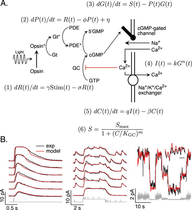
Model and fitting procedure.
(A) Phototransduction cascade and differential equations that describe the operation of key components. Abbreviations are as follows: Stim: stimulus; R: receptor (photopigment) activity; P: phosphodiesterase activity; G: cGMP concentration; S: rate of cGMP synthesis; I: membrane current; C: calcium concentration. (B) Fits (red) of a model with four free parameters (γ, σ, η, KGC) to the responses of a mouse rod (see Table 1). All measured responses are from the same rod, and all model responses use the same values for the free parameters. Responses to different flash strengths or flash timing have been displaced vertically in the left two panels. The weakest flash in the far left panel produced on average ~3 activated rhodopsin molecules, and each successive flash was twice as bright. The bottom trace in the middle panel was to a light step alone, while the other traces in this panel each had five superimposed flashes. The horizontal scale bar for the inset in B is 1 s.
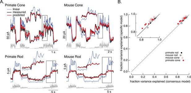
Photoreceptor model and fits.
(A) Comparison of measured responses (black) with predictions of full (red) and linear model (blue) to variable mean noise stimulus (gray). Full model responses used consensus parameters from fitting responses of multiple cells of each type simultaneously, with the dark current and sensitivity allowed to vary between cells (see Methods and Table 1). The linear model was generated from fitting the low-contrast responses of the full model (see Methods). Insets expand regions in gray boxes. Linear model parameters (see Equation 7) were α = 0.31, τR = 10.6 ms, and τD = 23.6 ms for the primate cone, α = 0.031, τR = 31.6 ms, and τD = 56.7 ms for the mouse cone, α = 5.3, τR = 141 ms, and τD = 208 ms for the primate rod, and α = 4.7, τR = 115 ms, and τD = 185 ms for the mouse rod, (B) Fraction of variance explained for the full model fit to each cell individually (y-axis) plotted against that for the consensus model that has fixed parameters across cells except for the dark current and sensitivity. Means ± SDs were 0.90 ± 0.04 (specific model) and 0.87 ± 0.05 (consensus model) for six primate cones, 0.92 ± 0.02 and 0.94 ± 0.02 for six mouse cones, 0.94 ± 0.02, 0.94 ± 0.02 and 0.94 ± 0.02 for six primate rods and 0.93 ± 0.03 and 0.93 ± 0.03 for eight mouse rods. Data for Figures 1-5 is available at https://doi.org/10.5061/dryad.q2bvq83vg.
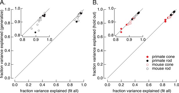
Tests of the ability of the model to generalize across stimuli and across cells.
(A) Generalization across stimuli. Responses of primate and mouse rods were fit to the variable mean noise stimulus only and model performance was evaluated for responses to the flash family and flashes and steps, using the fraction of variance explained to evaluate the fits (see Figure 1B). The generalization performance to stimuli not included in the fit (y-axis) is compared to performance when the model is fit to all stimuli (x-axis). Means ± SDs were 0.92 ± 0.05 (generalize) and 0.94 ± 0.03 (fit all) for six primate rods and 0.90 ± 0.04 and 0.92 ± 0.02 for eight mouse rods. (B) Generalization across cells. Models were fit to the variable mean noise stimulus. The performance of each cell was evaluated for a model in which all cells were fit (x-axis), or in which the test cell was excluded from the fit (y-axis). γ was allowed to vary for the held-out cell while other parameters were determined by fitting the remaining data as for the consensus models. Means ± SDs were 0.88 ± 0.04 (hold out) and 0.87 ± 0.05 (fit all) for six primate cones, 0.90 ± 0.02 and 0.91 ± 0.02 for six mouse cones, 0.96 ± 0.02 and 0.96 ± 0.02 for six primate rods, and 0.95 ± 0.02 and 0.95 ± 0.02 for eight mouse rods.
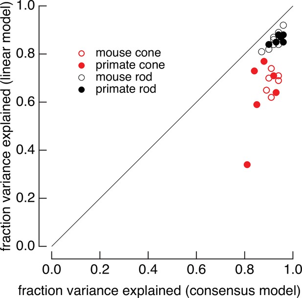
Full models systematically outperform linear models.
Linear models were generated by fitting low-contrast responses to the full model for each cell. Full models and linear models were optimized with a single-scale factor for each cell (γ for the full model and α for the linear model in Equation 7). The fraction of variance explained was computed for the variable mean noise stimuli as in Figure 2. Means ± SDs were 0.63 ± 0.15 (linear) and 0.87 ± 0.05 (consensus) for six primate cones, 0.68 ± 0.04 and 0.91 ± 0.02 for six mouse cones, 0.86 ± 0.02 and 0.96 ± 0.02 for six primate rods, and 0.86 ± 0.04 and 0.95 ± 0.02 for eight mouse rods.
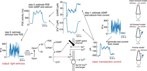
Steps in model inversion.
A test current was generated from a variable mean noise stimulus using the full model (far right). Step 1 (right) converts this current into changes in cGMP and calcium using Equations 4 and 5 (see Figure 1). Step 2 converts the time course of the cGMP and calcium into that of the phosphodiesterase (PDE) activity using Equations 3 and 6. Finally, step 3 converts the PDE to the stimulus using Equations 1 and 2. The estimated stimulus is identical to the initial stimulus because there is no added noise and the inversion process is exact. Icons at the far right depict different versions of the model used throughout the paper.
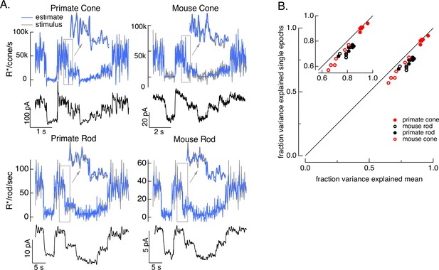
Test of model inversion based on measured responses.
(A) Stimulus (gray in top panel), measured response (black in lower panels), and estimated stimulus (blue in top panels) calculated by using the measured response as input to the inverse model as in Figure 3. Estimates are able to recover both the periodic changes in mean intensity and the more rapid superimposed stimulus modulations (insets). (B) Variance explained for stimulus estimates based on the average response across multiple stimulus trials compared to that based on individual responses. Since the model captures only the deterministic part of the response, noise in the individual responses lowers the accuracy of the estimates and causes the points to fall below the unity line. This effect is modest but systematic. Means ± SDs were 0.91 ± 0.02 (single epochs) and 0.92 ± 0.02 (mean) for six primate cones, 0.66 ± 0.08 and 0.72 ± 0.06 for six mouse cones, 0.74 ± 0.03 and 0.81 ± 0.04 for six primate rods, and 0.68 ± 0.04 and 0.77 ± 0.05 for eight mouse rods.
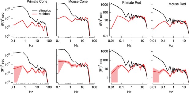
Errors in stimulus estimation.
Power spectra of stimulus and residual (stimulus − estimate) for example primate and mouse rods and cones (top) and averages across cells (bottom; six primate cones, six mouse cones, six primate rods, eight mouse rods). The stimulus and residual power spectra diverge strongly at low frequencies where the estimates are close to the actual stimulus, and converge at higher frequencies when the estimate becomes poor. The convergence point depends on photoreceptor type, as expected for the different kinetics of rod and cone responses.

Light-adaptation clamp procedure.
Starting with an initial stimulus (left), we generate a target or desired response (second panel from right).
In this case, the target was chosen to be the response of a linear phototransduction model; for a sinusoidal input, a linear model produces a sinusoidal output. We use the (linear) target response as the input to the inverse phototransduction model and identify the stimulus required to elicit that response (red in third panel from left). Substantial stimulus modifications are required for the full model to produce a sinusoidal output. Finally, we confirm that the modified stimulus works as designed in direct recordings, in this case from a primate cone (right panel). Linear model parameters used to compute the target response (see Equation 7) were α = 0.31, τR = 10.6 ms, and τD = 23.6 ms.
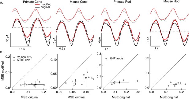
Compensating for increment/decrement asymmetries in responses to sinusoidal stimuli.
(A) Photoreceptor responses to original sinusoidal stimuli (bottom, black) and modified stimuli (red). Dashed lines in the bottom panels are best-fitting sinusoids for reference. Original and modified stimuli are shown above the recorded responses. Linear model parameters used to compute the target responses (see Equation 7) were α = 0.31 (20,000 R*/s) and 1.65 (5000 R*/s), τR = 10.6 and 15.2 ms, and τD = 23.6 and 18.1 ms for the primate cone, α = 0.031 and 0.13, τR = 31.6 and 26.7 ms, and τD = 56.7 and 50.3 ms for the mouse cone, α = 5.3, τR = 141 ms, and τD = 208 ms for the primate rod, and α = 4.7, τR = 115 ms, and τD = 185 ms for the mouse rod. (B) Mean-squared error between measured responses and best-fitting sinusoids for modified stimuli plotted against that for original stimuli for each recorded cell. Points with error bars are means ± SDs. These values are 0.15 ± 0.05 (modified) and 0.02 ± 0.02 (original) at 20,000 R*/s and 0.08 ± 0.06 and 0.03 ± 0.02 at 5000 R*/s for six primate cones, 0.10 ± 0.01 and 0.04 ± 0.03 (20,000 R*/s) and 0.06 ± 0.03 and 0.02 ± 0.01 (5000 R*/s) for five mouse cones, 0.14 ± 0.08 and 0.05 ± 0.01 for six primate rods, and 0.16 ± 0.04 and 0.03 ± 0.01 for seven mouse rods.
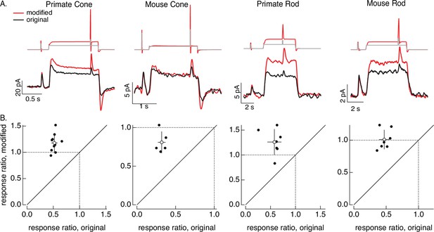
Compensating for adaptation produced by changes in mean light level.
(A) Responses to a brief light flash delivered before and during a step in light intensity. For the original stimuli, flashes delivered before and during the step are identical, and the resulting responses decrease in amplitude ~twofold (summarized on x-axis of bottom panels). Red traces show responses to stimuli designed to compensate for the adaptation produced by the change in light intensity (following approach in Figure 6). Linear model parameters used to compute the target responses (see Equation 7) were α = 1.65, τR = 15.2 ms, and τD = 18.1 ms for the primate cone, α = 0.13, τR = 26.7 ms, and τD = 50.3 ms for the mouse cone, α = 5.3, τR = 141 ms, and τD = 208 ms for the primate rod, and α = 4.7, τR = 115 ms, and τD = 185 ms for the mouse rod. (B) Summary of gain changes (amplitude of response during the step divided by that of response prior to step) for responses to modified (y-axis) and original (x-axis) stimuli. Open circles show the mean ± SD; values are 1.2 ± 0.2 (modified) and 0.52 ± 0.06 (original) for 10 primate cones, 0.8 ± 0.1 and 0.32 ± 0.05 for 5 mouse cones, 1.3 ± 0.3 and 0.6 ± 0.1 for 7 primate rods, and 1.0 ± 0.1 and 0.47 ± 0.08 for 7 mouse rods.
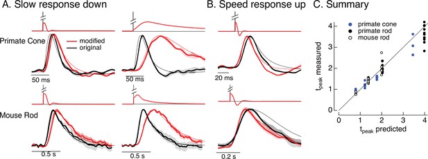
Manipulating kinetics of photoreceptor responses.
(A) Responses of primate cones and mouse rods to brief flashes (black) and stimuli designed to slow down responses slightly (left) and more substantially (right) (red). Traces show the mean ± SEM (four cells for upper left, three for upper right, five for both bottom panels). Thin traces show the target responses used to generate the modified stimuli. (B) As in A for stimuli designed to speed up responses (measured traces show mean ± SEM for four cones in the top panel and three rods in the bottom panel). (C) Measured change in time-to-peak plotted against predicted change for a variety of manipulations of kinetics as in A and B. Linear model parameters used to compute the target responses (see Equation 7) were α = 1.65, τR = 15.2 ms, and τD = 18.1 ms for the primate cone, α = 0.13, τR = 26.7 ms, and τD = 50.3 ms for the mouse cone, α = 5.3, τR = 141 ms, and τD = 208 ms for the primate rod, and α = 4.7, τR = 115 ms, and τD = 185 ms for the mouse rod.
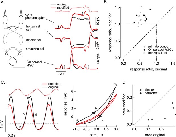
Cone and post-cone adaptation.
(A) Left: schematic of retinal circuit. Right: responses of a cone (top), horizontal cell (middle), and On parasol ganglion cell (bottom) to the step and flash protocol for both original and modified stimuli. Stimuli were delivered from a computer monitor at a refresh rate of 60 Hz and hence appear different from those in Figure 8. (B) Summary of experiments like those in A, plotting the change in gain for the modified stimuli (the ratio of the amplitude of the response to the flash during the step that before) against that for the original stimuli. Means ± SDs were 1.2 ± 0.2 (modified) 0.52 ± 0.06 (original) for 10 cones and 1.2 ± 0.1 and 0.6 ± 0.2 for 5 parasol RGCs. (C) Left: horizontal cell responses to a sinusoidal stimulus (black) and stimulus modified to generate sinusoidal cone responses (red, see also Figures 6 and 7). Right: trajectories of responses to one stimulus cycle. The response to the original stimulus follows different trajectories during the depolarizing (a→b→c) phase compared to the hyperpolarizing (c→d→a) phase. (D) Summary of results from three horizontal cells and three cone bipolar cells. Time-dependent nonlinearities were measured from the area enclosed by response trajectories as in C. Means ± SDs were 0.08 ± 0.05 (area modified) and 0.22 ± 0.08 (area original) across all six cells. Linear model parameters used to compute the target responses (see Equation 7) were α = 1.65, τR = 15.2 ms, and τD = 18.1 ms.
Tables
Parameters and best fit consensus values for biophysical phototransduction models for each cell type (see Methods for fitting details).
| Parameter | Symbol | Units | Type | Photoreceptor type | |||
|---|---|---|---|---|---|---|---|
| Primatecone | Mousecone | Primaterod | Mouserod | ||||
| Opsin decay rate const. | Free | 22 | 9.74 | 7.07 | 7.66 | ||
| PDE decay rate const. | Constrained (φ = σ) | 22 | 9.74 | 7.07 | 7.66 | ||
| PDE dark activation rate | η | Free | 2000 | 761 | 2.53 | 1.62 | |
| Dark current | pA | Measured | −240 to −428 | −41 to −80 | −19 to −37 | −16 to −24 | |
| cGMP concentration in dark | Derived | 28.7 to 35 | 15.9 to 20 | 12.1 to 15.0 | 11.4 to 13.1 | ||
| cGMP-to-current constant | k | Fixed | 0.01 | 0.01 | 0.01 | 0.01 | |
| cGMP channel cooperativity | n | Unitless | Fixed | 3 | 3 | 3 | 3 |
| Ca2+ concentration in dark | Fixed | 1 | 1 | 1 | 1 | ||
| Ca2+ extrusion rate constant | Fixed (rods) Free (cones) | 9 | 2.64 | 25 | 25 | ||
| Cooperativity of GC Ca2+ dependence | m | Unitless | Fixed | 4 | 4 | 4 | 4 |
| Affinity of GC Ca2+ dependence | Free | 0.5 | 0.4 | 0.5 | 0.4 | ||
| Opsin gain | Unitless | Free | 10 | 10 | 4.2 | 8 | |
| Reagent type (species) or resource | Designation | Source or reference | Identifiers | Additional information |
|---|---|---|---|---|
| Biological sample (Mus musculus) | 129S1/SvlmJ | The Jackson Laboratory | RRID:IMSR_JAX:002448 | |
| Biological sample (Mus musculus) | C57BL/6J | The Jackson Laboratory | RRID:IMSR_JAX:000664 | |
| Biological sample (Macaca fascicularis) | Washington Regional Primate Research Center | N/A | ||
| Biological sample (Macaca nemenstrina) | Washington Regional Primate Research Center | N/A | ||
| Chemical compound, drug | Ames | MilliporeSigma | Cat #A1420 | |
| Software, algorithms | MATLAB | Mathworks | https://www.mathworks.com/products/matlab.html | |
| Software, algorithms | Stage | Stage-VSS | https://stage-vss.github.io | |
| Software, algorithms | Symphony | Symphony-DS | http://symphony-das.github.io | |
| Software, algorithms | Igor Pro | Wavemetrics | N/A |
Parameter variations that double the mean-squared error of the fits.
Error was measured while a single parameter was systematically varied; other parameters were held fixed at the consensus model values.
| Parameter | Symbol | Units | Values: optimal [lower, upper] | |||
|---|---|---|---|---|---|---|
| Primatecone | Mousecone | Primaterod | Mouserod | |||
| Opsin decay rate const. | σ | 22 [14, 34] | 9.74 [7.3, 13.1] | 7.07 [5.8, 8.8] | 7.66 [6.1, 9.3] | |
| PDE dark activation rate | η | 2000 [1300, 3300] | 761 [494, 1218] | 2.53 [2.1, 3.2] | 1.62 [1.3, 2.1] | |
| Ca2+ extrusion rate const. | 9 [5, 40] | 2.64 [1.58, 5.7] | N.A. | N.A. | ||
| Ca2+ GC affinity | 0.5 [0, 0.6] | 0.4 [0.26 0.46] | 0.5 [0.44, 0.53] | 0.4 [0.32, 0.44] | ||


