Robust variability of grid cell properties within individual grid modules enhances encoding of local space
- Interdepartmental Graduate Program in Dynamical Neuroscience, University of California, Santa Barbara, United States
- Intelligent Systems Center, Johns Hopkins University Applied Physics Lab, United States
- Department of Neuroscience, The University of Texas at Austin, United States
- Center for Learning and Memory, The University of Texas at Austin, United States
- Center for Perceptual Systems, The University of Texas at Austin, United States
- Center for Theoretical and Computational Neuroscience, The University of Texas at Austin, United States
- Department of Psychological and Brain Sciences, University of California, Santa Barbara, United States
- Department of Molecular, Cellular, and Developmental Biology, University of California, Santa Barbara, United States
- Neuroscience Research Institute, University of California, Santa Barbara, United States
Figures
Figure 1
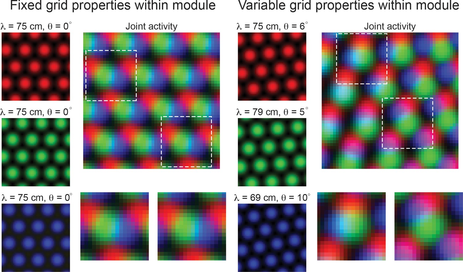
Variability in grid cell properties within a module leads to enhanced encoding of local space.
When the activity of three idealized grid cells, all with the same grid spacing and orientation, are considered, the periodicity of the responses limits the amount of information conveyed about local space (Left column – ‘Fixed grid properties within module’). That is, there are multiple locations in physical space with identical population level activity. However, when three grid cells with variable grid spacing and orientation (in the realm of what is measured within individual grid modules – see Results), their joint activity contains considerably more information (Right column – ‘Variable grid properties within module’). This benefit of spatial inhomogeneity is expected to increase with larger populations of grid cells. Dashed squares in the joint activity map are enlarged below.
Figure 2 with 1 supplement
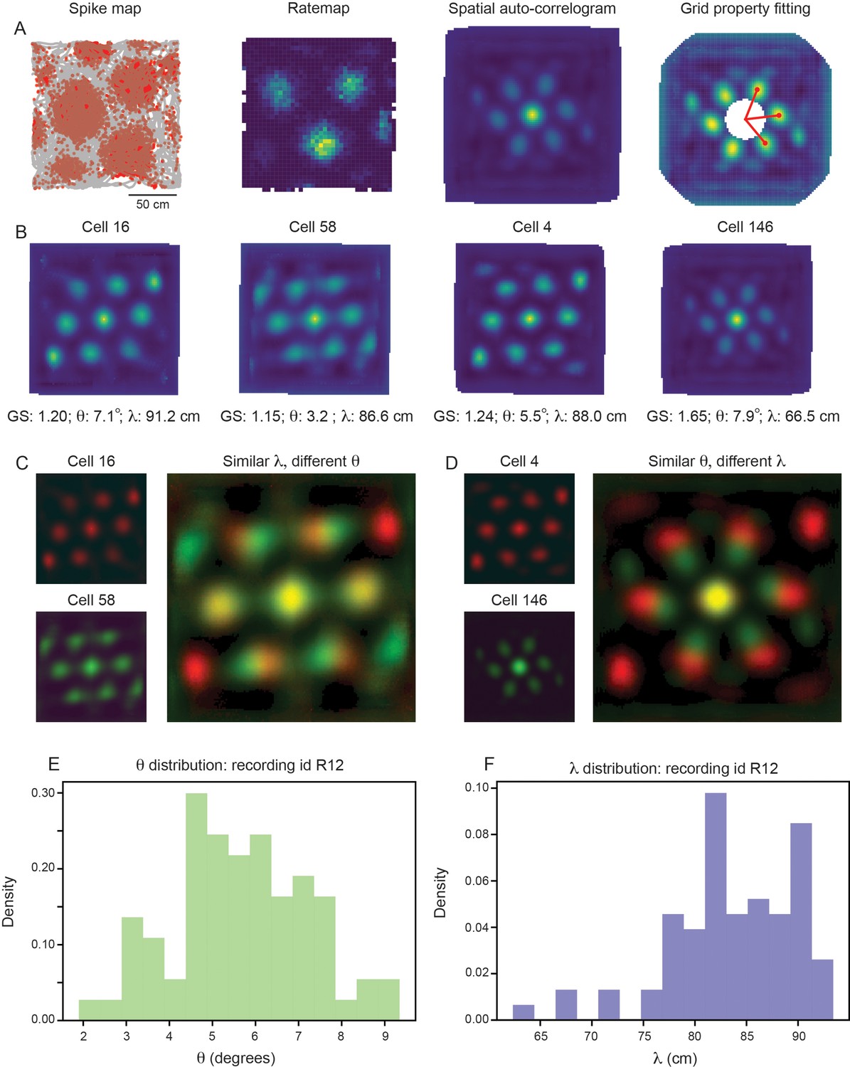
Grid properties are variable within a single grid module (recording ID R12).
(A) Overview of the standard procedure used to calculate the grid spacing and orientation of a given grid cell. First, spike maps are computed by identifying the location of the animal at the time of each spike. Gray line denotes the trajectory of the rat, red dots denote locations of spikes. A rate map is constructed by binning space and normalizing by the amount of time the rat spent in each spatial bin. A spatial autocorrelogram (SAC) is computed and, after the center peak is masked out (white pixels in the center of the spatial autocorrelogram – leading to change in color scale), the grid properties are fit by measuring the length and angle of the three peaks closest to 0°. (B) Example grid cells from the same module (recording ID R12), with estimated grid score, orientation (), and spacing (). (C, D) SAC overlaid for two pairs of grid cells (from B); one pair with different and similar (C) and the other with similar and different (D). (E, F) Distribution of (E) and (F) across all grid cells with grid score >0.85 (N=74).
Figure 2—figure supplement 1
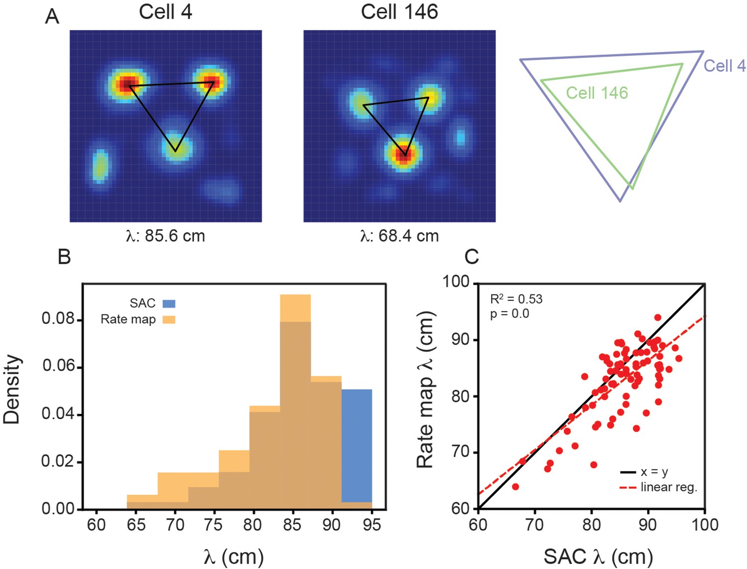
Variability in grid spacing within a single module exists when computing directly from the rate maps.
(A) (Left) Example grid cell rate maps from the same module (recording ID R12) with overlaid triangles, corresponding to the spacing between each of the three most central peaks. Grid spacing is computed as the average of the three lengths. (Right) To aid comparison, the triangles are enlarged (with their relative size fixed) and overlaid. Note that these cells are the same ones plotted in Figure 2B. (B) Distribution of grid spacing computed using the SAC and the rate maps. (C) The grid spacing of all grid cells, from recording R12, computed using the SAC and the rate map. Red dashed line is the linear regression fit with and p-value reported above.
Figure 3 with 7 supplements
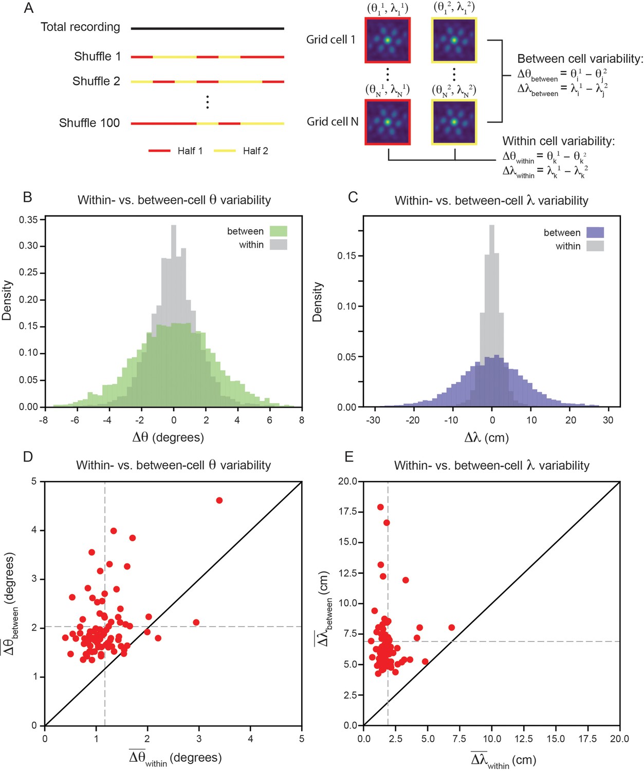
Variability of grid properties is a robust feature of individual grid module (recording ID R12).
(A) Schematic overview of approach used to compute the between- and within-cell variability of grid orientation and spacing. (B, C) Distribution of within- and between-cell variability of and , respectively. Note that the distribution is across all 100 random shuffles of the data into two halves. (D) Average within-cell variability of grid orientation (), compared to average between-cell variability of grid spacing (). (E) Same as (D), but for . 1 cell was excluded from (E) for visualization (), but was included in non-parametric statistical analysis. For (D, E), .
Figure 3—figure supplement 1
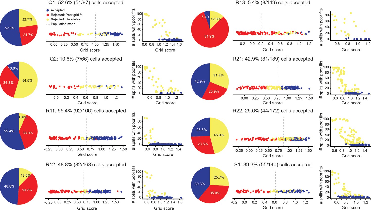
Accepted and rejected cells across all grid modules.
(Left) The percent of all cells, across all modules, that were rejected by our inclusion criteria. Cells that were rejected as not having SACs, computed with all data, that were well described by hexagonal structure (‘Rejected: Poor grid fits’) are shown in red. Cells that were rejected as not reliably having SACs, computed from splits of the data, that were well described by hexagonal structure (‘Rejected: Unreliable’) are shown in yellow. Cells that met these criteria (‘Accepted’) are shown in blue. (Middle) Grid score of all cells, with coloring denoting whether they were accepted or rejected. Dashed gray line denotes population mean. (Right) The number of splits of the data (out of 100) that cells had SAC’s with poor grid fits, as a function of each cell’s grid score.
Figure 3—figure supplement 2
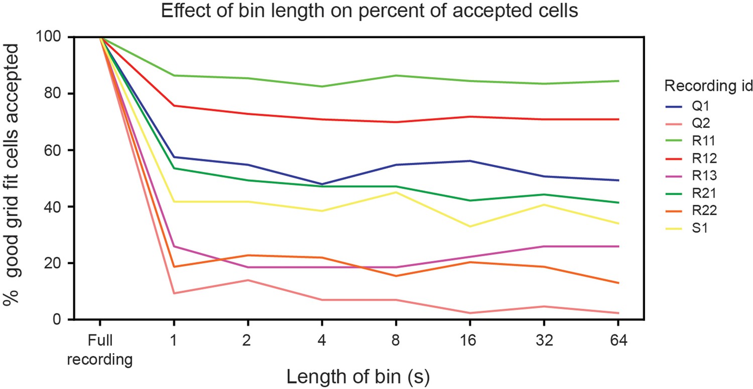
Bin length does not affect the percent of cells accepted for analysis.
The percent of cells with good grid fits (i.e. those cells that do not get rejected for having ‘poor grid fits’) that are accepted by not being deemed unreliable, as a function of the size of the bins used in the shuffle analysis. All modules are plotted (each line is colored based on its recording ID).
Figure 3—figure supplement 3

Average field width does not play a significant role in explaining the between-cell variability in spacing.
(A) Schematic illustration of how the average field width was approximated. The first minima along 1-dimensional slices through the center of the SAC are used to estimate the field width. (B) An example ratemap with the four strongest grid fields overlaid with circles having the diameter of the estimated field width. (C) Between-cell spacing variability () as a function of average field width for all cells from recording R12 that passed our inclusion criteria. Red line is the linear regression fit with and p-value reported. , for all other modules: Q1 = 0.06; Q2 = 0.40; R11 = 0.04; R13 = 0.03; R21 = 0.12; R22 = 0.12; S1 = 0.00.
Figure 3—figure supplement 4
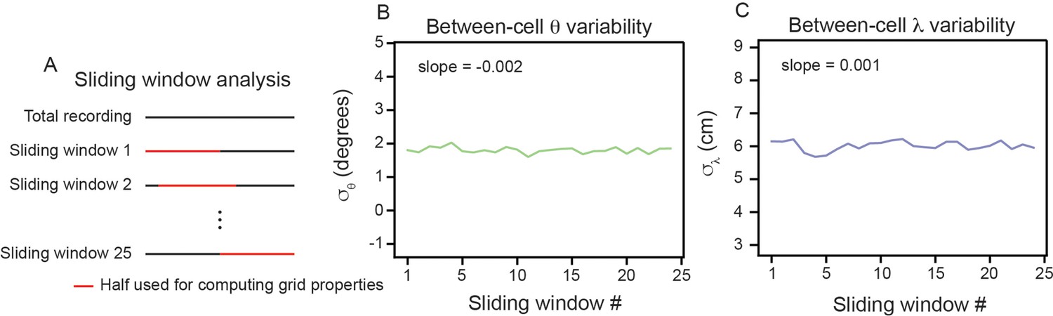
Between-cell variability does not significantly change across recording time.
(A) Schematic illustrating the sliding window analysis. Red line denotes half of data used to compute the grid properties. (B, C) Between-cell variability (estimated by computing the standard deviation of the population and values) as a function of sliding window number. The slope estimated from a linear regression fit is reported. Slope in and , for all other modules: Q1 = 0.015 and 0.028; Q2 = –0.039 and 0.003; R11 = –0.001 and –0.005; R13 = 0.005 and –0.000; R21 = 0.014 and 0;.020; R22 = 0.044 and 0.016; S1 = 0.034 and 0.014.
Figure 3—figure supplement 5
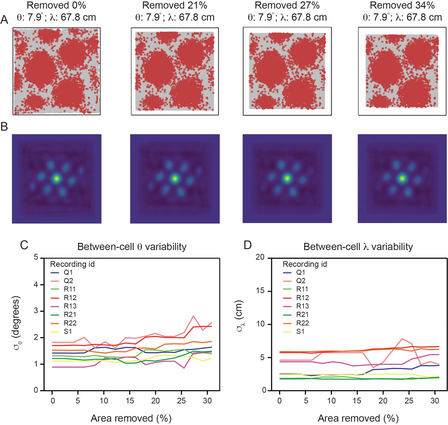
Variability in grid spacing and orientation is not significantly affected by location of arena boundaries.
(A) Example spike map for one cell (from R12) as increasingly more of the arena is removed. Computed and are reported above the spike maps. (B) SACs corresponding to the spike maps. (C, D) Between-cell variability (estimated by computing the standard deviation of the population and values) as a function of how much of the arena was removed from our analysis for all modules.
Figure 3—figure supplement 6
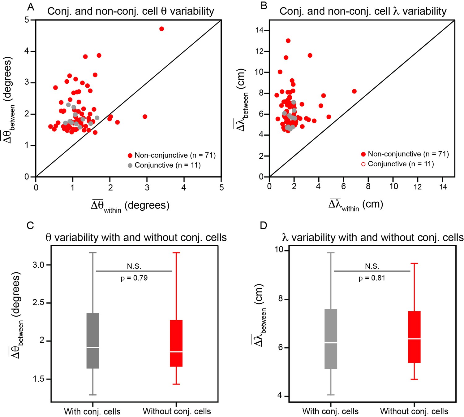
Conjunctive head direction grid cells do not significantly affect the variability in grid orientation and spacing.
(A, B) Same as Figure 2D and E, but with conjunctive and non-conjunctive cells differentiated. Note that the slight difference in position of the dots between this figure and Figure 3 is due to re-computing with a different random seed. (C, D) Distribution of between-cell variability in orientation and spacing, when computing and with and without the conjunctive cells. To allow paired comparisons, the variability is calculated for only the non-conjunctive cells, but either includes (grey) or does not include (red) variability comparisons to the conjunctive cells. A paired t-test is used to determine whether the distributions are significantly different (p-values reported in C, D). P-value in and , for all other modules: Q1 = 0.65 and 0.78; Q2 = 0.86 and 0.92; R11 = 0.13 and 0.75; R13 = 0.99 and 0.97; R21 = 0.29 and 0.98; R22 = 0.87 and 0.95; S1 = 0.07 and 0.77.
Figure 3—figure supplement 7
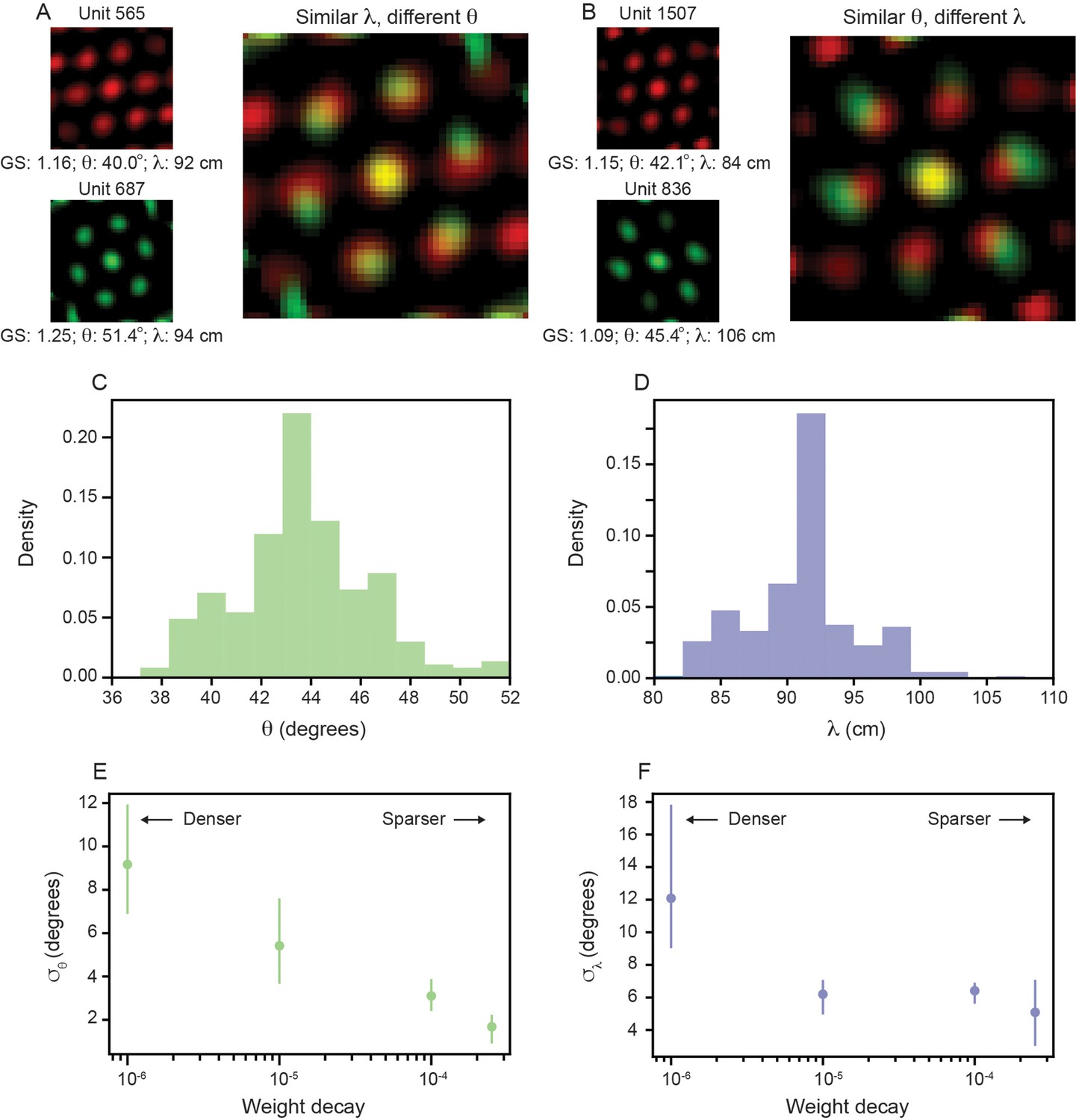
Path integrating recurrent neural networks (RNNs) that develop grid cells exhibit variability in spacing and orientation that scales with recurrent weight sparsity.
(A, B) Spatial autocorrelogram (SAC) overlaid for two pairs of units in the recurrent layer with high grid score; one pair with different and similar (A) and the other with similar and different (B). (C, D) Distribution of (C) and (D) across all units in the recurrent layer with grid score > 0.85 (N = 326). Two and four units were excluded for visualization from (C) and (D), respectively, since they were outside the plotting axes. (E, F) Standard deviation of (E) and (F) distributions, and respectively, across different amounts of weight decay used in training. The circle markers indicate the mean across three independently trained networks and the lines indicate the minimum and maximum of all three networks.
Figure 4
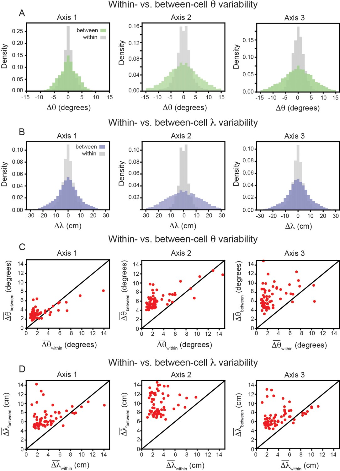
Variability of grid properties, restricted to the same axis, is a robust feature of individual grid module (recording ID R12).
Same analysis as in Figure 3B–E, but for variability measured on each axis independently. (A) Distribution of orientation variability (Δθ) for each grid axis. (B) Distribution of spacing variability (Δλ) for each grid axis. (C) Within- vs. between-cell orientation variability () for each grid axis. (D) Within- vs. between-cell spacing variability () for each grid axis. For visualization, we exclude a small number of cells that were outside the axes limits, including 2, 5, and 10 cells for Axes 1–3, respectively (C); and 3, 4, and 3 cells for Axes 1–2, respectively (D); these cells were included in non-parametric statistical analyses.
Figure 5
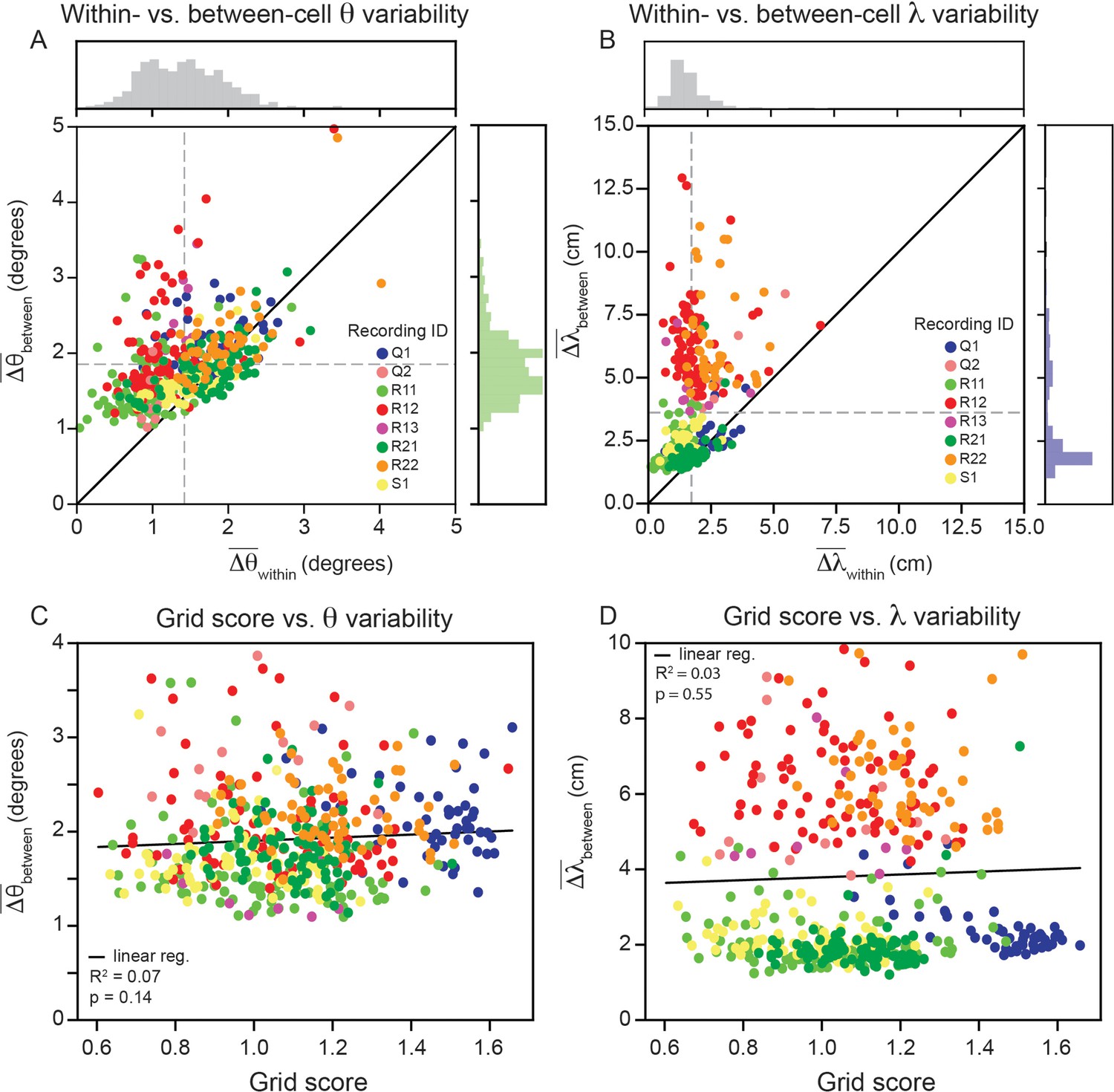
Within module grid property variability is a robust feature across modules.
(A) Average within-cell variability of grid orientation (), compared to average between-cell variability of grid orientation () for each cell () across 8 modules (cells colored by their corresponding recording ID). The histogram above the plot shows the distribution of and the histogram to the right shows the distribution of . (B) Same as (A), but for grid spacing. For visualization, 5 cells are excluded (), but are included in non-parametric statistical analyses. Dashed gray lines show the population mean. (C, D) Average within cell variability of and (respectively), as a function of grid score. For visualization, 3 and 22 cells are excluded from (C, D), respectively, but are included in statistical analyses. Black solid line is linear regression, with and p-value reported above.
Figure 6 with 2 supplements
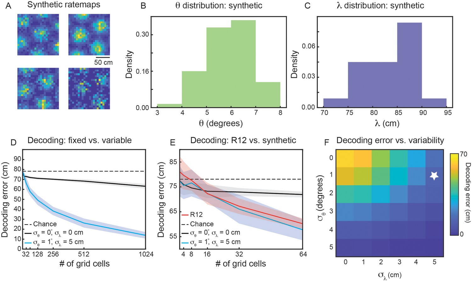
Variability in grid properties enables improved decoding of local space from the activity of grid cells within a single module.
(A) Example noisy grid cell rate maps generated from a Poisson process. The size of the square arena is set to 1.5 m ×1.5 m to be consistent with what was used in the experimental set-up analyzed (Gardner et al., 2022). (B, C) Distribution of sampled grid spacing and orientation from synthetic population, when using , , cm, and ; compare to the distribution measured from real data (Figure 2E and F). (D) Decoding error, as a function of grid cell population size, with populations having either no variability in grid properties (black line) or variability similar to what was present in the data analyzed (blue line). The solid line is the mean across 25 independent grid cell populations and the shaded area is ± standard deviation of the 25 independent populations. The dashed black line shows chance level decoding error. (E) Decoding error for synthetic populations and real data for up to cells (red line). (F) Decoding error, over a grid of and values, for populations of grid cells. White star denotes values used in (D).
Figure 6—figure supplement 1
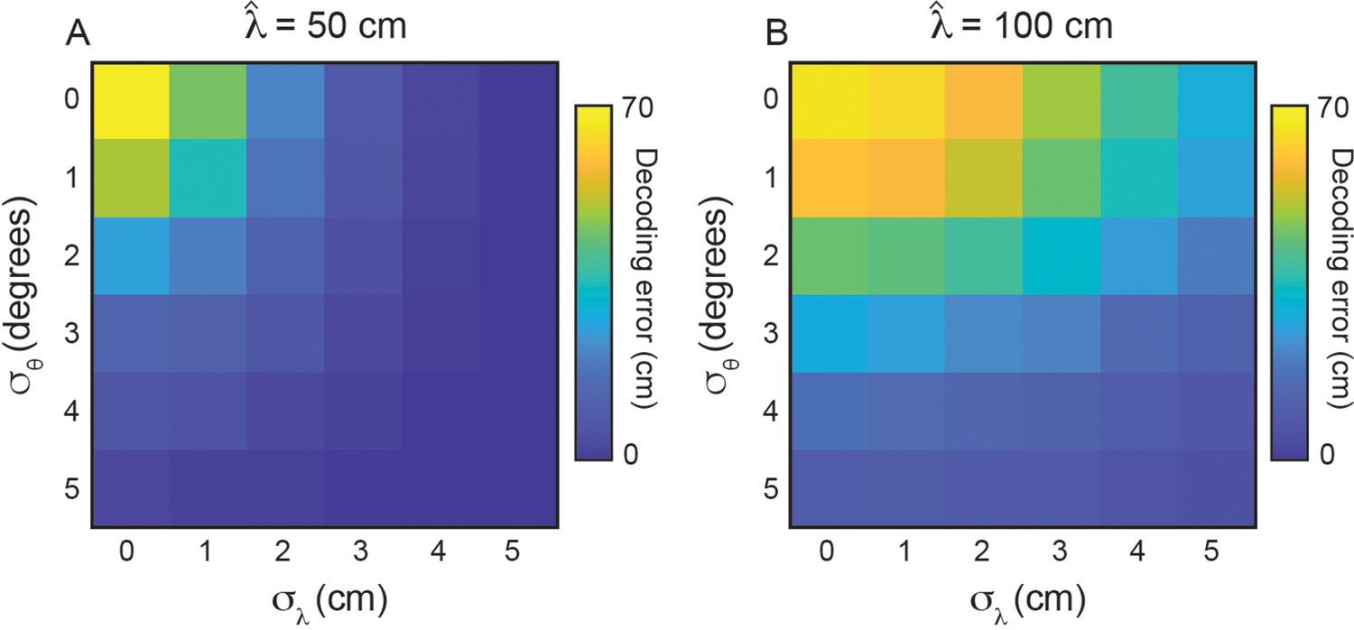
Variability in grid properties improves decoding of local space for grid modules with different mean grid spacings.
(A, B) Same as Figure 6F, for cm and cm, respectively. is set to 0°.
Figure 6—figure supplement 2
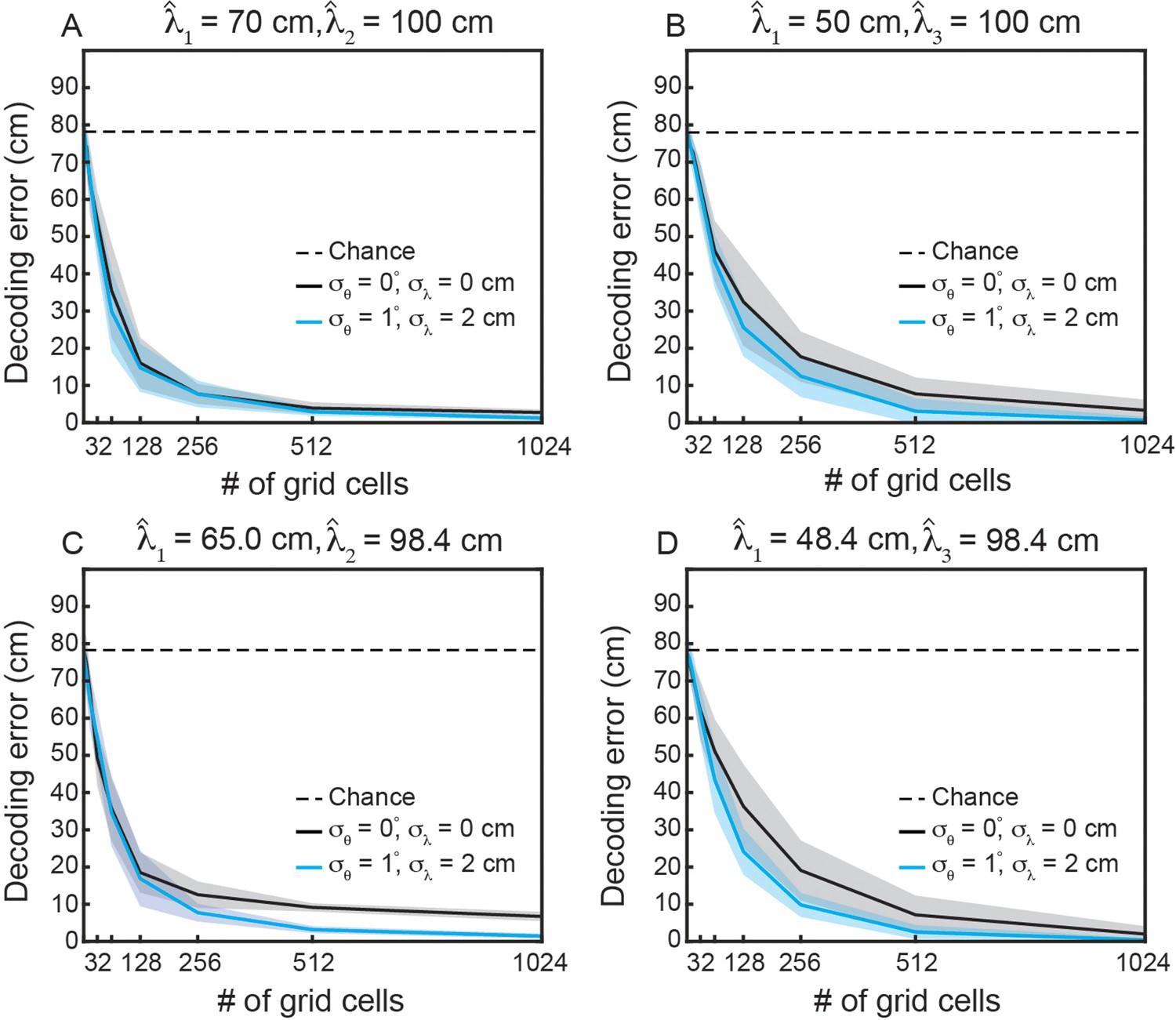
Variability in grid properties improves decoding of local space for multiple modules, when the modules have integer multiple mean spacing.
(A–D) Same as Figure 6D, when decoding from multiple modules. (A) and . (B) and . (C) and (D) and . The values in (A, B) were chosen such that and . The values in (C, D) were chosen to match those found in Rat 14257 from Stensola et al., 2012.
Author response image 1

Grid propertied along Axis 1 are not less variable for many recorded grid modules.
Same as Fig.4C-D, but for four other recorded modules. Note that the variability along each axis is similar.
Tables
Table 1
Parameters used to train RNNs on path integration.
See Sorscher et al., 2019; Sorscher et al., 2023 for more information on these parameters.
| Parameter | Value |
|---|---|
| Epochs | 100 |
| Batch size | 200 |
| Batches per epoch | 1000 |
| Path length (T) | 20 |
| Arena length (L) | 2.2m |
| Learning rate | 10-4 |
| Place cells (np) | 512 |
| Grid cells (nG) | 2096 |
| 0.12 | |
| 0.24 | |
| Activation | ReLU |
| Weight decay | 10-4 |
| Optimizer | Adam |
Additional files
Download links
A two-part list of links to download the article, or parts of the article, in various formats.
Downloads (link to download the article as PDF)
Open citations (links to open the citations from this article in various online reference manager services)
Cite this article (links to download the citations from this article in formats compatible with various reference manager tools)
Robust variability of grid cell properties within individual grid modules enhances encoding of local space
eLife 13:RP100652.
https://doi.org/10.7554/eLife.100652.3


