Standardized mean differences cause funnel plot distortion in publication bias assessments
- University Medical Center Utrecht, Netherlands
- Netherlands Heart Institute, Netherlands
- University of Edinburgh, United Kingdom
- University of Tasmania, Australia
- Radboud University Medical Center, Netherlands
Figures
Figure 1
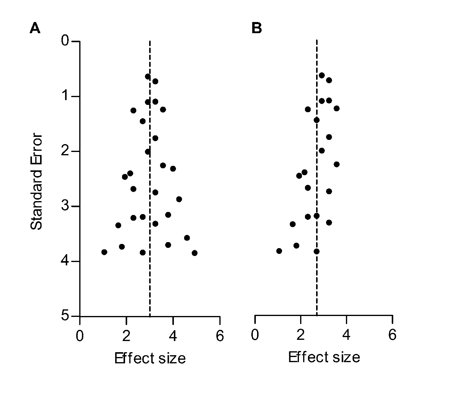
Hypothetical funnel plots in the absence (A) and presence (B) of bias.
The precision estimate used is the standard error (SE). Dashed lines indicate the summary effect estimate.
Figure 2
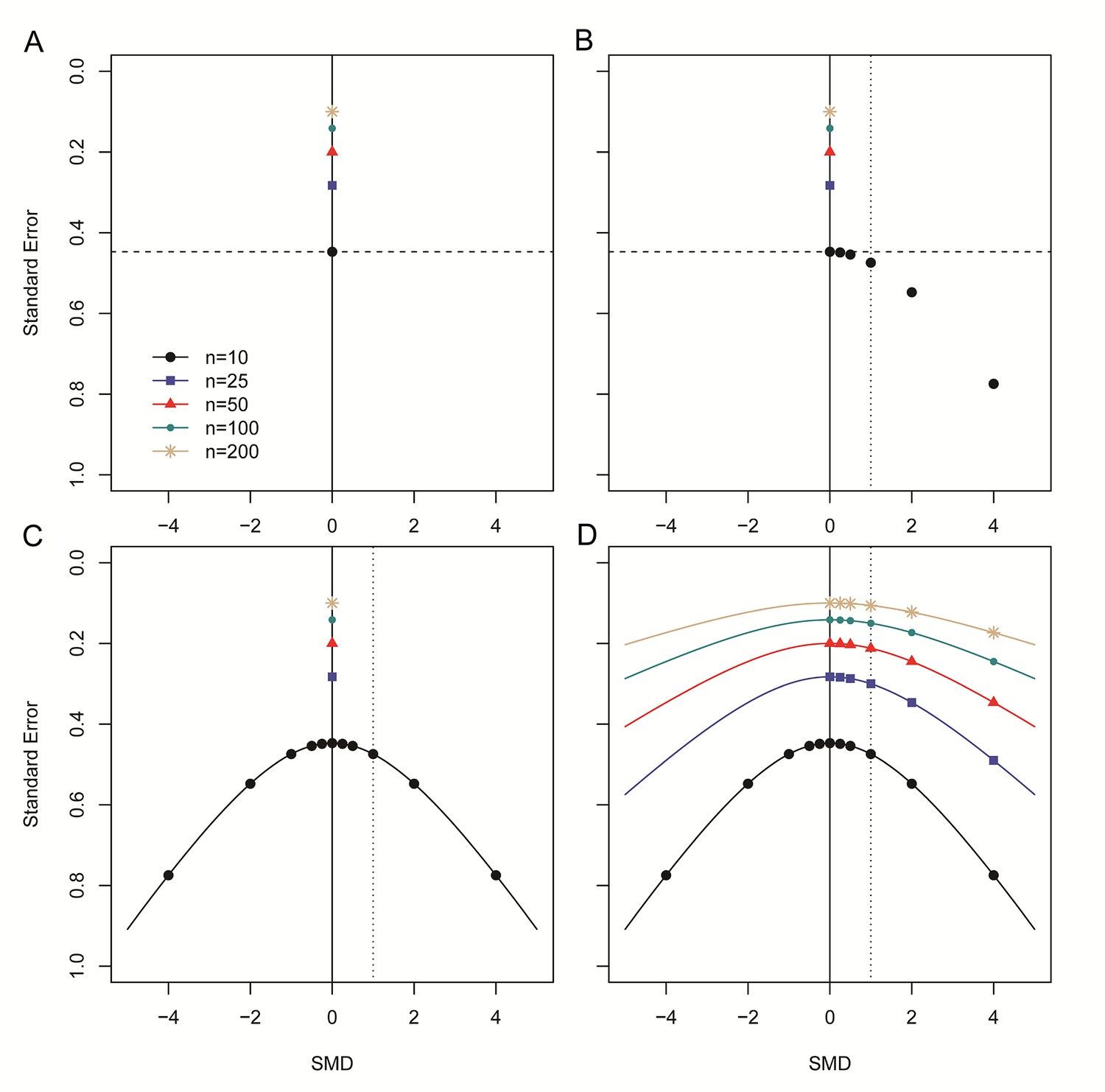
Step-wise illustration of distortion in SMD versus SE funnel plots.
(A) Depicted are simulated studies with a sample size of respectively 10 (large black circles), 25 (blue squares), 50 (red triangles), 100 (small green circles) and 200 (gold asterisks) subjects per group, and an SMD of zero. The SE of these studies (indicated by the dashed line for studies with n = 10) solely depends on their sample size, as SMD2 = 0 and therefore does not contribute to the equation for the SE. As expected, the SE decreases as the sample size increases. (B) Five data points from simulated studies with n = 10 and a stepwise increasing SMD are added to the plot. For these studies, the SMD2 contributes to the equation for the SE, and the SE will decrease even though the sample size is constant. The dotted line represents a hypothetical summary effect of SMD = 1 in a meta-analysis. Note that when assessing a funnel plot for asymmetry around this axis, the data points with an SMD < 1 have skewed to the upper left-hand region, whereas studies with an SMD > 1 are in the lower right region of the plot. This distortion worsens as the SMD increases. (C) Because the SMD is squared in the equation for the SE, the same distortion pattern is observed for negative SMDs. Thus, funnel plots will be distorted most when the study samples sizes are small and SMDs are either very positive or very negative. (D) The same deviation is observed for simulated studies with larger sample sizes, however, the deviation decreases as the sample size increases, because the sample size will outweigh the effect of SMD2 in the equation for the SE.
Figure 3
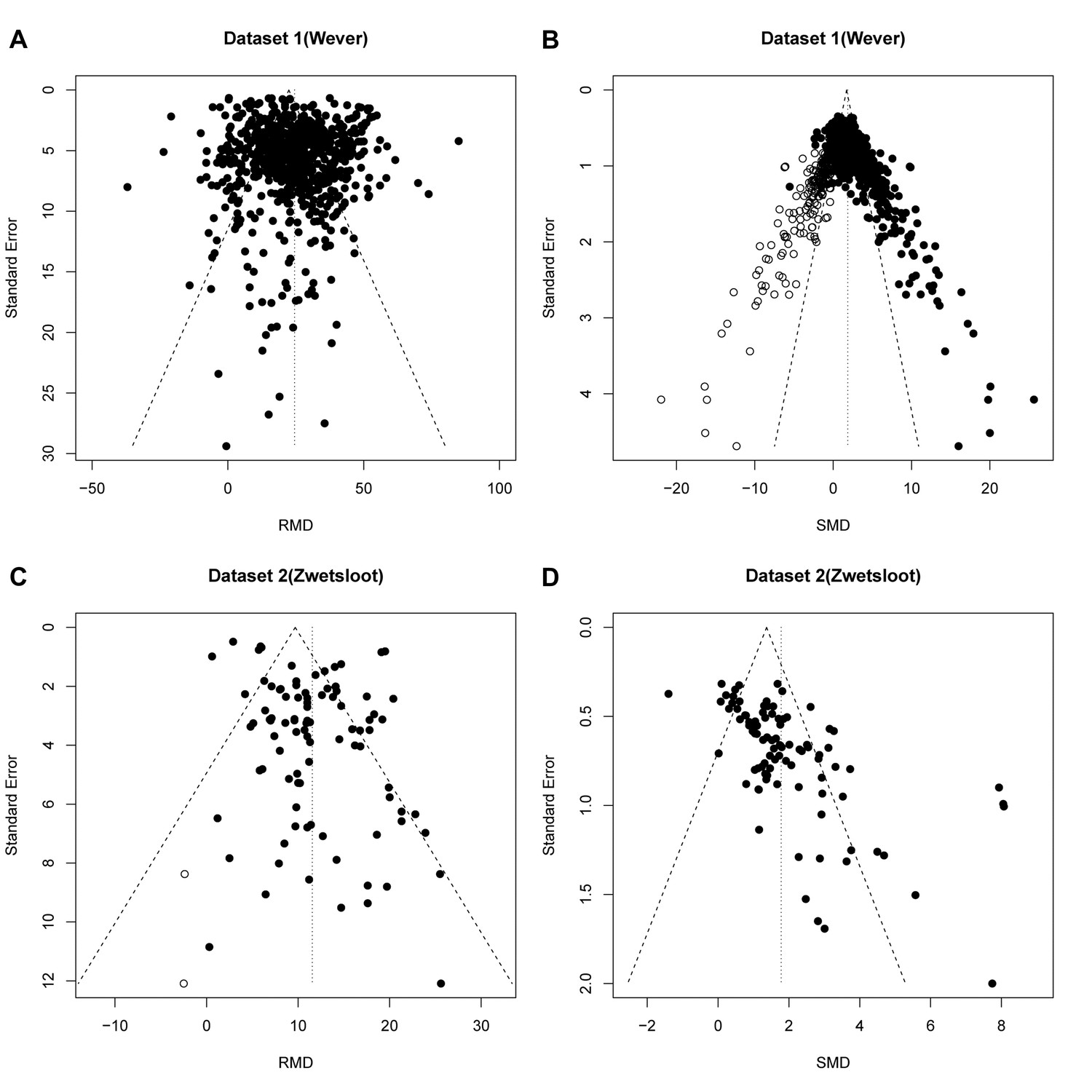
Reanalysis of data from Wever et al.
(A,B) and Zwetsloot et al. (C,D), with funnel plots based on raw mean difference (RMD; A,D) or standardized mean difference (SMD; B,D). Filled circles = observed data points; open circles = missing data points as suggested by trim and fill analysis.
Figure 4 with 2 supplements
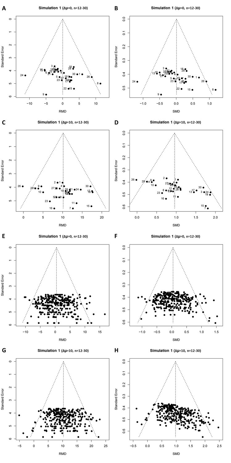
Representative raw mean difference (RMD; A, C, E, G) and standardized mean difference (Hedges’ g SMD; B, D, F, H) funnel plots for simulated unbiased meta-analyses containing thirty (A–D) or 300 (E–H) studies with a small sample size (total study n = 12–30).
Simulations were performed without an intervention effect (Δμ = 0; A–B and E–F), or with an intervention effect (Δμ = 10; C–D and G–H). Δμ = difference in normally distributed means between control and intervention group. Representative funnel plots for studies with a large sample size (total study n = 60–320) are shown in Figure 4—figure supplement 1. Representative funnel plots for the comparison between Hedges’ g and Cohen’s d are shown in Figure 4—figure supplement 2.
Figure 4—figure supplement 1
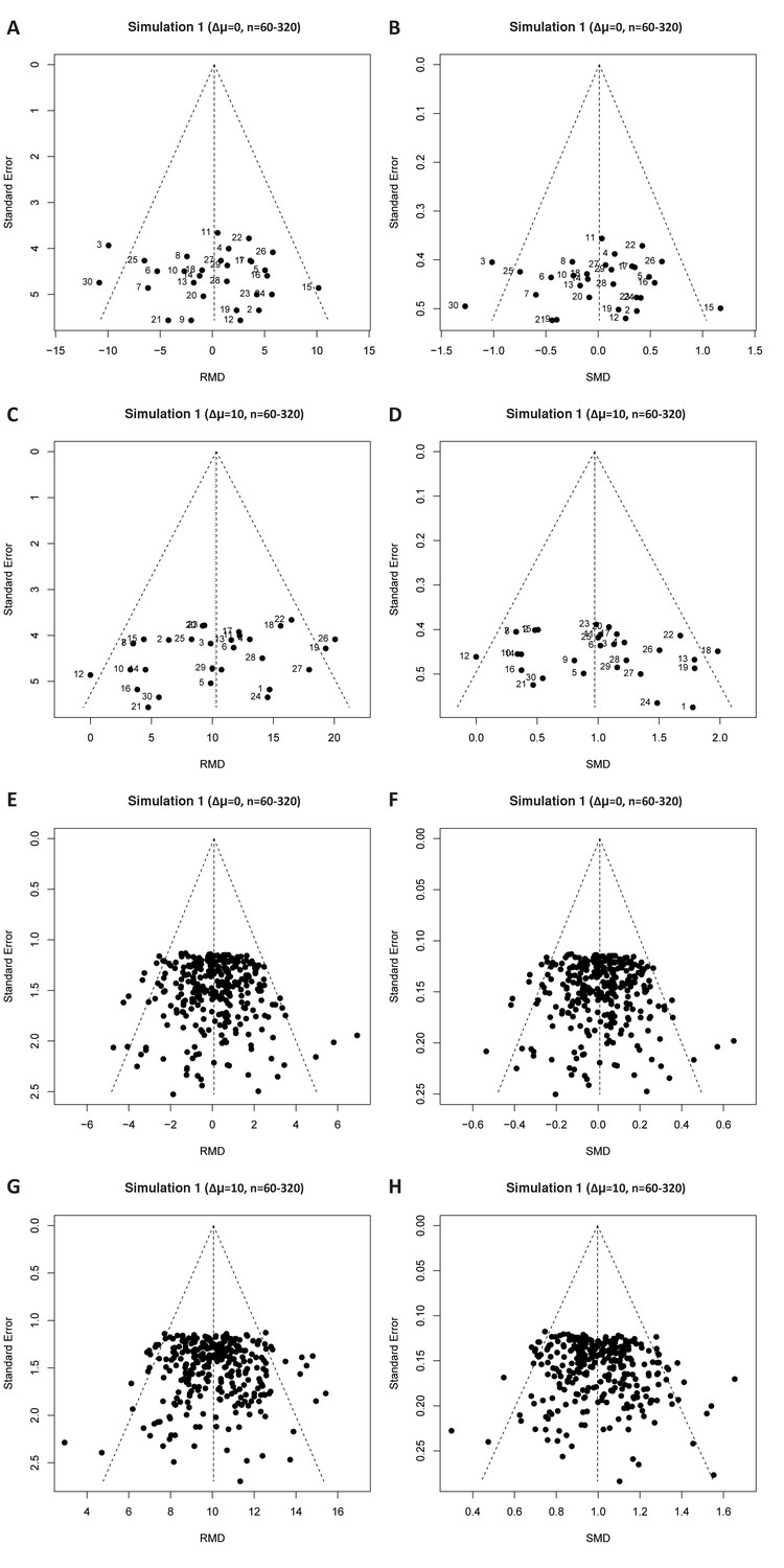
Simulation 1 funnel plots for large study sample sizes.
https://doi.org/10.7554/eLife.24260.006
Figure 4—figure supplement 2
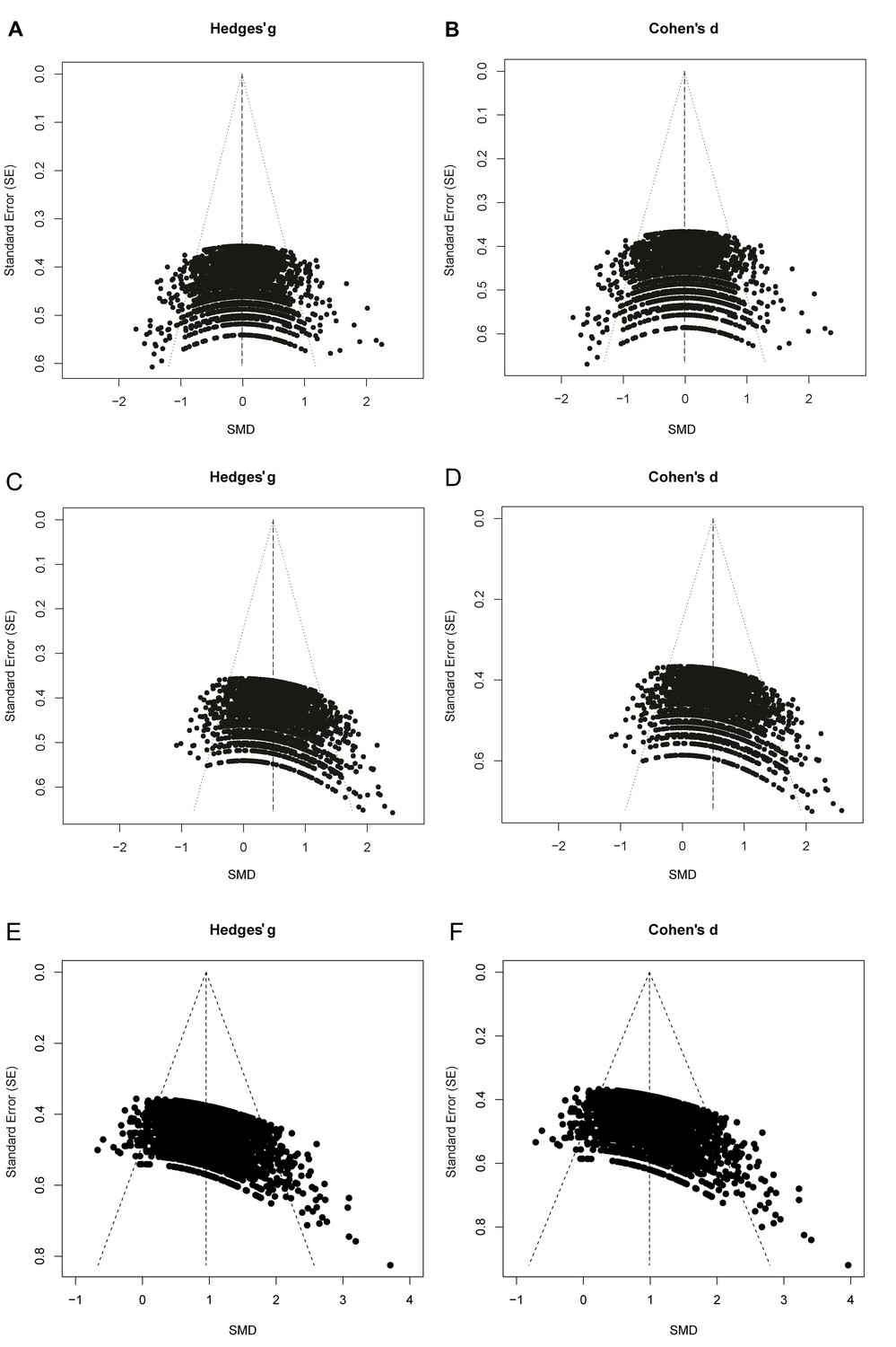
Funnel plots comparing Cohen’s d versus Hedges g.
https://doi.org/10.7554/eLife.24260.007
Figure 5
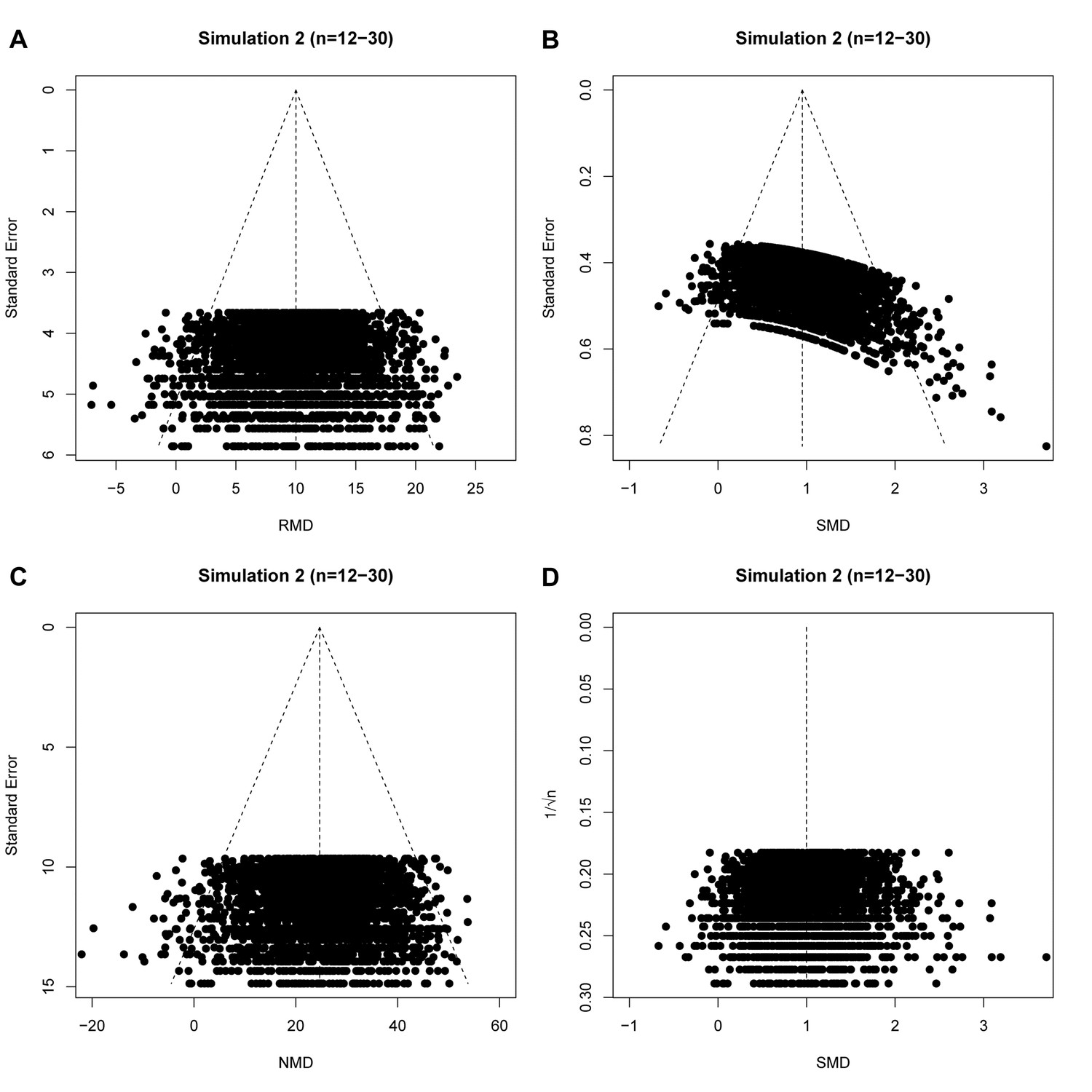
raw mean difference (RMD; A), standardized mean difference (SMD; B), normalized mean difference (NMD; C) with SE as precision estimate, and SMD funnel plots using 1/√n as precision estimate (D).
All plots show the same simulated meta-analysis containing 3000 studies with small sample sizes (n = 12–30) and an overall intervention effect of Δμ = 10. Δμ = difference in normally distributed means between control and intervention group.
Figure 6

Simulation 3 funnel plots of biased meta-analyses.
Representative funnel plots of simulated biased meta-analyses using a raw mean difference (RMD; A–B), a standardized mean difference (SMD; C–D), or a normalised mean difference (NMD; E–F) effect measure. The present example contains 3000 studies with a small study sample size (n = 12–30) and an intervention effect present (difference in normal distribution means between control and intervention group = 10). Publication bias was introduced stepwise, by removing 10% of primary studies in which the difference between the intervention and control group means was significant at p<0.05, 50% of studies where the significance level was p≥0.05 to p<0.10, and 90% of studies where the significance level was p≥0.10. Precision estimates are standard error (A, C, E) or sample size-based (B, D, F), where n = total primary study sample size.
Figure 7
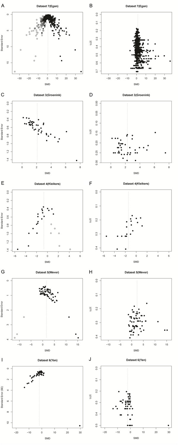
Funnel plots of re-analysis of empirical meta-analyses.
Funnel plots of empirical meta-analyses plotted as standardized mean difference (SMD) versus standard error, as in the original publications (left hand panels), and as SMD versus 1/√n after re-analysis. n = total primary study sample size; filled circles = observed data points; open circles = missing data points as suggested by trim and fill analysis.
Tables
Table 1
Study characteristics in relation to publication bias assessment in simulation of unbiased meta-analyses (simulation 1)
https://doi.org/10.7554/eLife.24260.008| Total study N | Δμ | No. of studies in MA | Effect measure | % of simulations with Egger’s p<0.05 | No. of studies filled by T&F (mean(min - max)) | Overall effect size (mean(min - max)) | Overall effect size after T&F (mean(min - max)) |
|---|---|---|---|---|---|---|---|
| 12–30 | 0 | 30 | RMD | 6.2% | 2.1 (0–11) | 0.74(−12.2–11.3) | 0.0(−3.8–3.6) |
| SMD(g) | 9.3% | 1.6 (0–10) | 0.1(−1.1–1.4) | 0.0(−0.36–0.33) | |||
| 12–30 | 5 | 30 | RMD | 4.9% | 2.1 (0–10) | 5.3(−3.4–19.1) | 5.0 (1.2–9.6) |
| SMD(g) | 19.5% | 2.4 (0–10) | 0.55(−0.4–2.2) | 0.43 (0.11–0.74) | |||
| 12–30 | 10 | 30 | RMD | 4.6% | 2.0 (0–10) | 11.2 (1.2–20.4) | 10.0 (5.4–13.5) |
| SMD(g) | 67.2% | 4.4 (0–10) | 1.16 (0.2–2.4) | 0.85 (0.5–1.2) | |||
| 12–30 | 0 | 300 | RMD | 4.8% | 25.4 (0–62) | 0.0(−15.2–12.3) | 0.0(−2.1–2.3) |
| SMD(g) | 9.8% | 18.8 (0–57) | 0.0(−1.9–1.6) | 0.0(−0.2–0.2) | |||
| 12–30 | 5 | 300 | RMD | 5.5% | 25.1 (0–65) | 5.5(−10.2–23.7) | 5.0 (3.0–6.8) |
| SMD(g) | 96.0% | 47.3 (0–70) | 0.55(−1.1–2.3) | 0.37 (0.28–0.50) | |||
| 12–30 | 10 | 300 | RMD | 5.9% | 25.8 (0–61) | 10.3(−11.1–29.0) | 10.0 (7.9–12.3) |
| SMD(g) | 100% | 61.5 (40–76) | 1.0(−1.4–3.1) | 0.80 (0.70–0.89) | |||
| 12–30 | 0 | 3000 | RMD | 5.4% | 249 (0–453) | 0.0(−18.6–17.9) | 0.0(−1.4–1.3) |
| SMD(g) | 8.7% | 175.1 (0–386) | 0.0(−2.1–2.6) | 0.0(−0.1–0.1) | |||
| 12–30 | 5 | 3000 | RMD | 4.4% | 252 (0–475) | 4.9(−13.0–21.1) | 5.0 (3.7–6.4) |
| SMD(g) | 100% | 492(417 - 565) | 0.49(−1.7–2.9) | 0.36 (0.33–0.39) | |||
| 12–30 | 10 | 3000 | RMD | 5.0% | 250 (0–456) | 10.0(−7–27) | 10.0 (8.6–11.3) |
| SMD(g) | 100% | 620(568 - 669) | 1.0(−0.7–4.5) | 0.79 (0.8–0.8) | |||
| 60–320 | 0 | 30 | RMD | 4.7% | 2.4 (0–10) | −0.2(−3.8–3.3) | 0.0(−1.3–1.3) |
| SMD(g) | 5.0% | 2.4 (0–10) | 0.0(−0.4–0.4) | 0.0(−0.1–0.1) | |||
| 60–320 | 5 | 30 | RMD | 3.8% | 2.2 (0–10) | 4.8 (1.9–7.6) | 5.0 (3.8–6.1) |
| SMD(g) | 5.2% | 2.4 (0–13) | 0.48 (0.2–0.8) | 0.5 (0.4–0.6) | |||
| 60–320 | 10 | 30 | RMD | 5.9% | 2.4 (0–10) | 10.0 (6.7–14.0) | 10.0 (8.7–11.2) |
| SMD(g) | 7.9% | 2.6 (0–10) | 1.0 (0.6–1.3) | 1.0 (0.8–1.1) | |||
| 60–320 | 0 | 300 | RMD | 4.4% | 18.9 (0–58) | 0.1(−3.7–5.5) | 0.0(−0.5–0.6) |
| SMD(g) | 4.6% | 17.3 (0–58) | 0.0(−0.4–0.5) | 0.0(−0.1–0.1) | |||
| 60–320 | 5 | 300 | RMD | 4.7% | 17.8 (0–63) | 4.9 (0.0–9.7) | 5.0 (4.4–5.6) |
| SMD(g) | 11.8% | 20.7 (0–60) | 0.49 (0.0–0.9) | 0.49 (0.4–0.5) | |||
| 60–320 | 10 | 300 | RMD | 6.2% | 18.4 (0–63) | 10.1 (4.8–16.5) | 10.0 (9.4–10.6) |
| SMD(g) | 33.9% | 29.5 (0–71) | 1.0 (0.5–1.7) | 0.97 (0.9–1.0) | |||
| 60–320 | 0 | 3000 | RMD | 5.3% | 140.0 (0–367) | 0.0(−6.5–5.6) | 0.0(−0.3–0.3) |
| SMD(g) | 5.4% | 136.6 (0–348) | 0.0(−0.7–0.6) | 0.0 (0.0–0.0) | |||
| 60–320 | 5 | 3000 | RMD | 4.7% | 143 (0–331) | 5.0(−1.4–11.3) | 5.0 (4.7–5.3) |
| SMD(g) | 69.0% | 243 (0–391) | 0.5(−0.1–1.2) | 0.48 (0.46–0.51) | |||
| 60–320 | 10 | 3000 | RMD | 5.0% | 135.8 (0–340) | 10.0 (4.6–16.2) | 10.0 (9.7–10.3) |
| SMD(g) | 99.7% | 334.5(168–464) | 1.0 (0.47–1.61) | 0.97 (0.95–0.98) |
-
n = sample size; Δμ = difference in normally distributed means between intervention and control group; no. = number; MA = meta analysis; T and F = trim and fill analysis; RMD = raw mean difference; SMD(g)=Hedges’ g standardized mean difference; SD = standard deviation
Table 2
publication bias assessments in unbiased and biased simulations using the RMD, SMD or NMD in combination with an SE or sample size-based precision estimate (simulation 3).
https://doi.org/10.7554/eLife.24260.009| Precision estimate SE | Precision estimate 1/√n | ||||
|---|---|---|---|---|---|
| Effect measure | Bias? | % of sims with Egger’s p<0.05 | Median p-value (range) | % of sims with Egger’s p<0.05 | Median p-value (range) |
| RMD | No | 5.1 | 0.51 (0.001–1.0) | 5.1% | 0.50 (0.001–1.0) |
| RMD | Yes | 69.1% | 0.01 (2.7*10−8 - 0.99) | 69.6% | 0.01 (1.6*10−8 - 0.97) |
| SMD | No | 100% | 2.9*10−13(0–8.1*10−6) | 4.3% | 0.51 (0.001–1.0) |
| SMD | Yes | 100% | 4.4*10−16(0–1.8*10−6) | 72.4% | 0.01 (5.4*10−10 - 0.99) |
| NMD | No | 6.4% | 0.51 (0.001–1.0) | 6.4% | 0.50 (0.001–1.0) |
| NMD | Yes | 60.5% | 0.02 (7.1*10−8 - 0.99) | 60.4% | 0.02 (8.0*10−8 - 0.98) |
-
Simulated meta-analyses contained 300 studies (total study n = 12–30 subjects) and the difference in normally distributed means between control and intervention group was 10. Publication bias was introduced stepwise, by removing 10% of primary studies in which the difference between the intervention and control group means was significant at p<0.05, 50% of studies where the significance level was p≥0.05 to p<0.10, and 90% of studies where the significance level was p≥0.10. SE = standard error; RMD = raw mean difference; SMD = standardized mean difference (Hedges’ g); NMD = normalized mean difference; sims = simulations.
Table 3
Re-analysis of published preclinical meta-analyses using SMD
https://doi.org/10.7554/eLife.24260.012| Precision estimate | ||||||||
|---|---|---|---|---|---|---|---|---|
| Standard Error | 1/√n | |||||||
| Study | n | Observed SMD[95% CI] | Egger’s p | filled | Adjusted SMD | Egger’s p | filled | Adjusted SMD |
| Egan et al. (2016) | 1392 | 0.75 [0.70, 0.80] | <2.2×10⁻¹⁶ | 252 | 0.42 [0.37,0.47] | 2.2 × 10⁻¹¹ | 0 | N/A |
| Groenink et al. (2015) | 43 | −1.99[−2.33,–1.64] | 8.5 × 10⁻¹⁰ | 0 | N/A | 0.68 | 0 | N/A |
| Kleikers et al. (2015) | 20 | −1.15[−1.67; −0.63] | 3.5 × 10⁻⁴ | 6 | ? | 2.9 × 10⁻³ | 0 | N/A |
| Wever et al. (2012) | 62 | 1.54 [1.16, 1.93] | 7.8 × 10⁻⁶ | 3 | ? | 0.62 | 0 | N/A |
| Yan et al. (2015) | 60 | 1.58 [1.19, 1.97] | 6.5 × 10⁻⁶ | 0 | N/A | 0.19 | 0 | N/A |
-
n = number of studies; SMD = standardized mean difference; CI = confidence interval; Egger’s p=p value for Egger’s regression; adjusted SMD = SMD after trim and fill analysis; N/A = not applicable.
Table 4
Simulation characteristics.
https://doi.org/10.7554/eLife.24260.014| Small studies | Large studies | RMD | SMD | NMD | |||||
|---|---|---|---|---|---|---|---|---|---|
| Experimental groups | N | Mean | SD | N | Mean | SD | |||
| Intervention 1 (no effect) | 7–14 | 30 | 10 | 40–150 | 30 | 10 | 0 | 0 | 0 |
| Intervention 2 (RMD = 5) | 7–14 | 35 | 10 | 40–150 | 35 | 10 | 5 | 0.5 | 0.125 |
| Intervention 3 (RMD = 10) | 7–14 | 40 | 10 | 40–150 | 40 | 10 | 10 | 1 | 0.25 |
| Control | 5–16* | 30 | 10 | 20–170* | 30 | 10 | |||
| Sham | 4–6 | 70 | 4 | ||||||
-
n = sample size; ND = normal distribution; SD = standard deviation; *control group sample size = intervention group sample size ±≤2 (small studies) or ±≤20 (large studies).
Additional files
-
Supplementary file 1
Cohen’s d and Hedges’ g, as well as Egger’s test and Begg and Mazumdar’s test, perform similar in multiple illustrative scenario’s (simulation 1).
- https://doi.org/10.7554/eLife.24260.015
-
Supplementary file 2
Supplemental equations.
- https://doi.org/10.7554/eLife.24260.016
-
Supplementary file 3
R scripts.
- https://doi.org/10.7554/eLife.24260.017
-
Transparent reporting form
- https://doi.org/10.7554/eLife.24260.018
Download links
A two-part list of links to download the article, or parts of the article, in various formats.
Downloads (link to download the article as PDF)
Open citations (links to open the citations from this article in various online reference manager services)
Cite this article (links to download the citations from this article in formats compatible with various reference manager tools)
Standardized mean differences cause funnel plot distortion in publication bias assessments
eLife 6:e24260.
https://doi.org/10.7554/eLife.24260


