Genetic and environmental perturbations lead to regulatory decoherence
- Princeton University, United States
- University of California, San Francisco, United States
- University of California, Los Angeles, United States
- Tampere University, Finland
- Tampere University, Tampere University Hospital, Finland
- University of Turku, Finland
- Turku University Hospital, Finland
- Systems Epidemiology, Baker Heart and Diabetes Institute, Australia
- University of Oulu, Finland
- University of Eastern Finland, Finland
- University of Bristol, United Kingdom
- The Alfred Hospital, Monash University, Australia
Figures
Figure 1 with 2 supplements
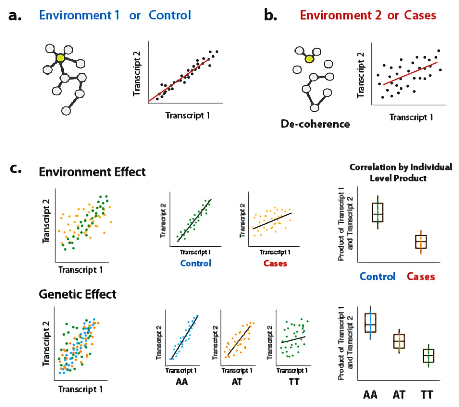
Illustration of decoherence and ‘Correlation by Individual Level Product’ (CILP).
(a) Co-expression networks in two different environments. Environment one represent normal (or control/baseline) conditions where the expression levels of gene 1 and gene 2 are highly correlated and co-regulated. (b) Environment 2 represents a stressful or unhealthy condition leading to lower correlation between the expression levels of gene 1 and gene 2. At the network level, this translates into a lower network degree (i.e., lower average correlation across genes or fewer connected nodes). We call this change in the correlation structure 'decoherence'. This is what we could expect if stressful conditions lower transcriptional robustness and lead to dysregulation of gene expression. (c) Differences in correlation between the expression levels of gene 1 and gene 2 in cases versus controls, or between genotypes, which translates into an average difference in product between these groups.
Figure 1—figure supplement 1
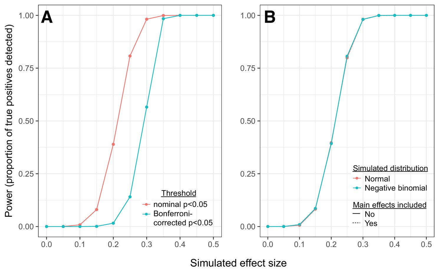
Simulations reveal power to detect correlation QTLs across a range of effect sizes.
(A) Power to detect correlation QTLs as a function of the simulated effect size and the significance cutoff. Each point represents the results from 10,000 pairs of simulated traits, across 1,000 individuals; effect sizes represent the degree to which samples originating from different genotypic classes exhibit different levels of correlation for each trait pair (higher effect sizes = larger differences in correlation between each genotypic class). For each simulated set of 10,000 pairs, we tested for correlation QTL using the approach described in the main text. (B) Comparison of simulation results: 1) when a multivariate normal distribution was used to simulate pairs of continuous trait values; 2) when a negative binomial distribution was used to simulate pairs of count data; and 3) when data were simulated as in 1, but mean gene expression levels for each gene in a given pair were included as covariates in linear models testing for correlation QTL.
Figure 1—figure supplement 2
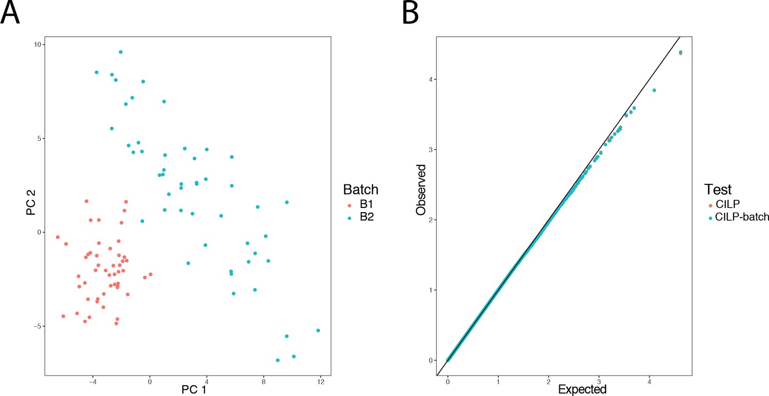
Simulated batch effects on transcriptional correlation structure do not produce false positive correlation QTLs.
500 genes were simulated in 100 individuals over two batches, with no covariance between genes in batch 1, and a covariance of 0.3 among all pairs of genes in batch 2. Panel A presents a PCA on the simulated gene expression data, with individuals colored by batch. To assess the false positive rate under the null, a genotype was simulated with no effect, and CILP was applied to estimate the genetic effect on the degree of correlation between each gene pair. Panel B shows that the observed p-values from CILP both when adjusting for batch (by including it as a covariate in a linear model) as well as ignoring batch are not greater than p-values observed under the expected uniform distribution, suggesting that batch effects do not cause inflation or affect the estimation of the genetic effect.
Figure 2 with 1 supplement
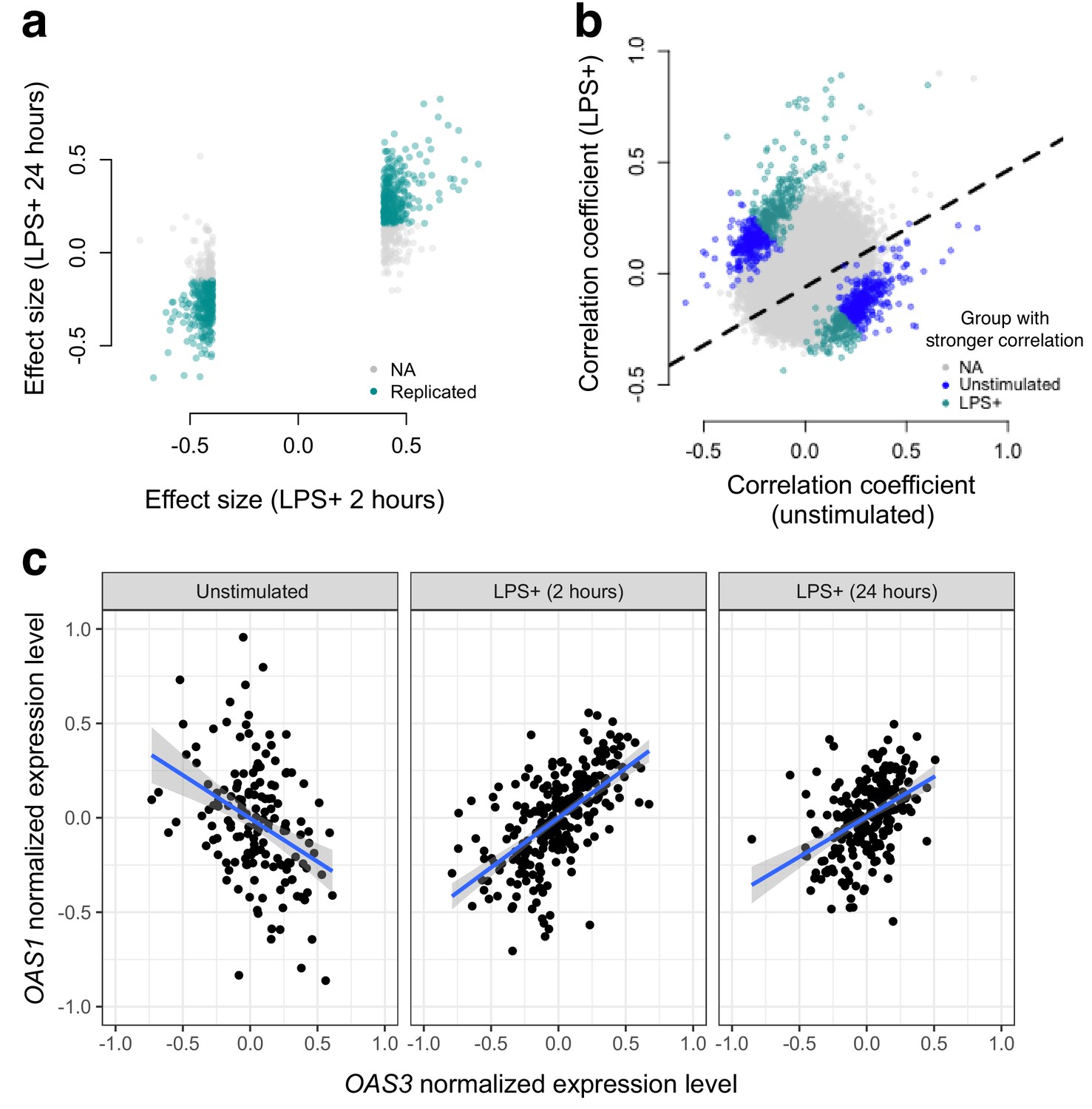
Bacterial infection (i.e., treatment with LPS) leads to decoherence in primary monocyte gene expression.
(a) Correlation changes have similar effect sizes after 2 hr or 24 hr of LPS stimulation. (b) Comparison of the Spearman correlation coefficient estimated in unstimulated cells (x-axis) versus those treated with LPS (y-axis). Gene pairs for which we detect significantly stronger correlations in the unstimulated (blue dots) or LPS treated (green dots) condition are highlighted. (c) An example of changes in correlation as a function of condition. Gene expression levels for OAS1 and OAS3 are negatively correlated at baseline, but become positively correlated after 2 hr or 24 hr treatment with LPS.
Figure 2—figure supplement 1
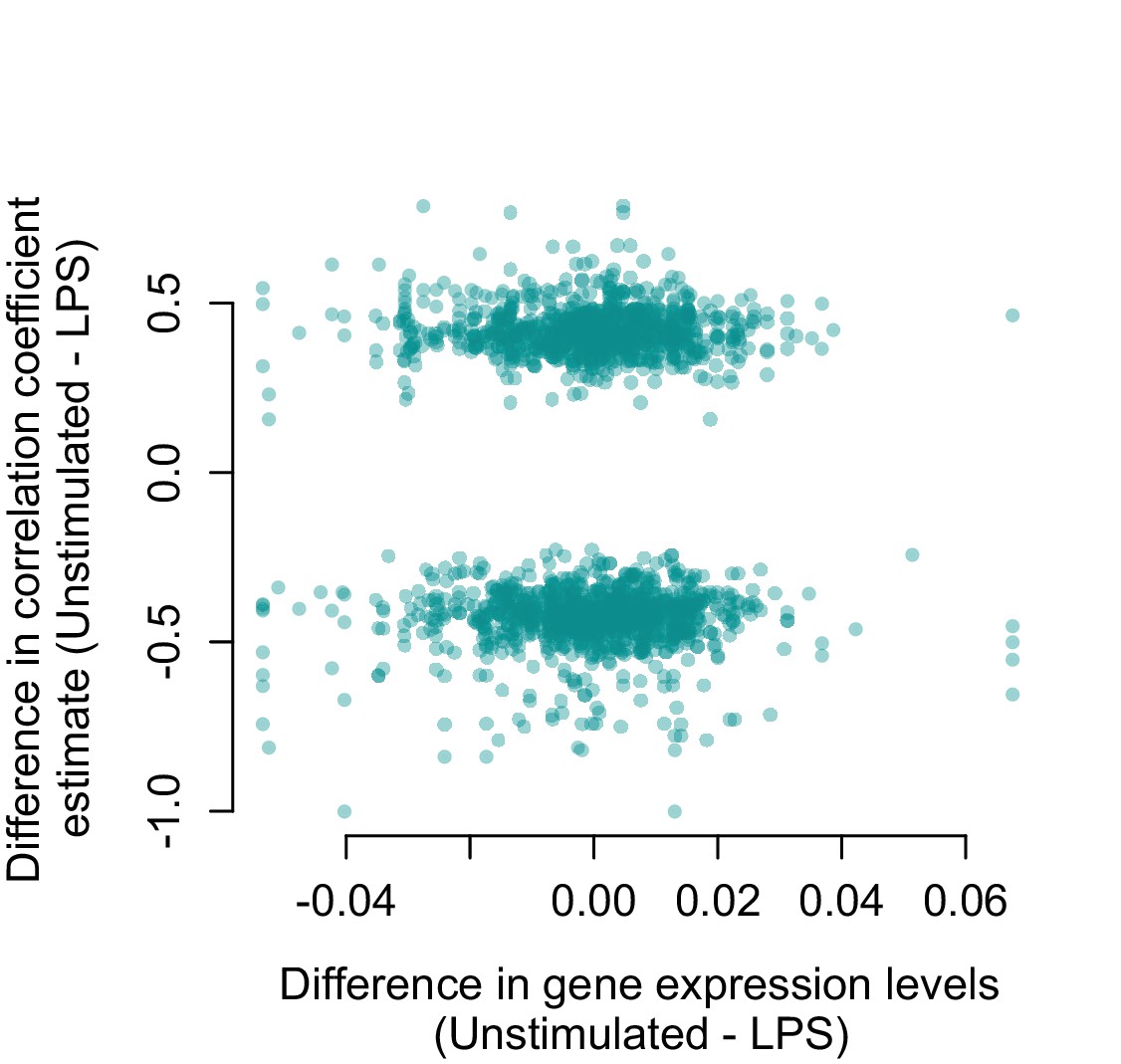
Genes that are strongly differentially expressed between conditions (unstimulated versus LPS 2 hr) are not more likely to change their correlation structure.
For all gene pairs that significantly increased or decreased in correlation following LPS stimulation, there is no relationship between the difference in mean normalized gene expression levels measured in unstimulated cells versus LPS stimulated cells (x-axis) and the magnitude of the correlation change (y-axis; R2 = 2.38×10⁻⁴, p=0.499).
Figure 3 with 1 supplement
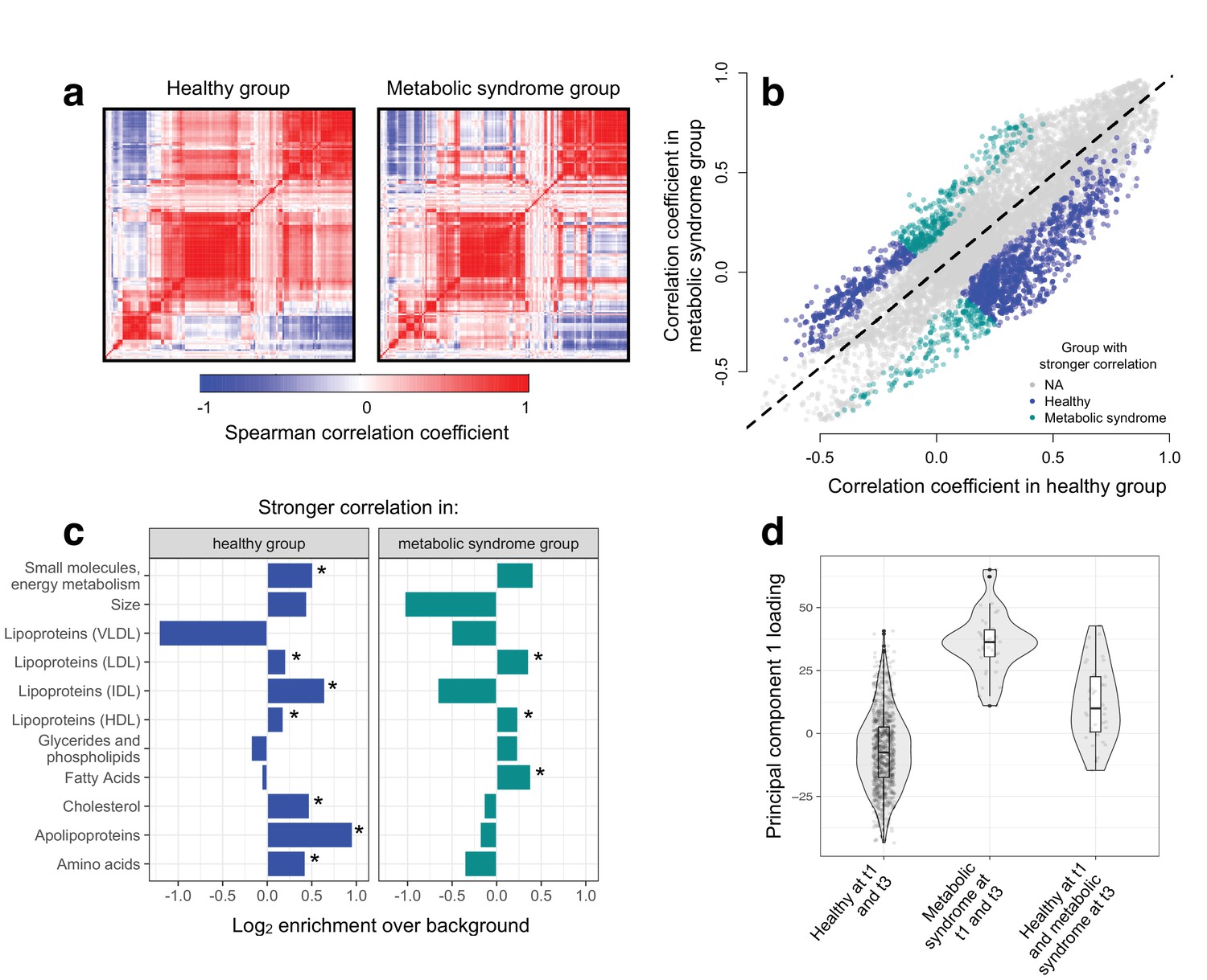
Metabolic syndrome leads to decoherence among particular metabolite pairs.
(a) Correlation matrices showing the magnitude of the Spearman correlation coefficient, for healthy individuals and those with metabolic syndrome. (b) Comparison of the Spearman correlation coefficient estimated in healthy individuals (x-axis) versus those with metabolic syndrome (y-axis). Overall, the magnitude of the correlation is similar between groups (R2 = 0.62, p<10−16), though the slope of the line is already less than 1, indicating a tendency toward stronger correlations in healthy individuals (beta = 0.814). For the subset of metabolite pairs that display significantly stronger correlations in the healthy (blue dots) or metabolic syndrome class (green dots), this effect is more pronounced (beta = 0.597). (c) Categorical enrichment of metabolites that exhibit stronger pairwise correlations in the healthy or metabolic syndrome class (x-axis: log2 odds ratio from a Fisher’s exact test; y-axis: 11 functional classes tested (annotations taken from (Nath et al., 2017)). Asterisks indicate significant enrichment. (d) A composite measure of metabolites that are strongly decoherent at the first time point (i.e., that show decreases in correlation in individuals with metabolic syndrome) can predict an individual’s future health status. Y-axis: Principal component 1 of 34 metabolites, measured at the first time point, with the strongest evidence for dysregulation. X-axis: values are stratified by whether an individual was healthy at the first (t0) and the last (t3) time point, had metabolic syndrome at t0 and t3, or developed metabolic syndrome between t0 and t3 (linear model, p=3.03×10⁻¹⁰).
Figure 3—figure supplement 1
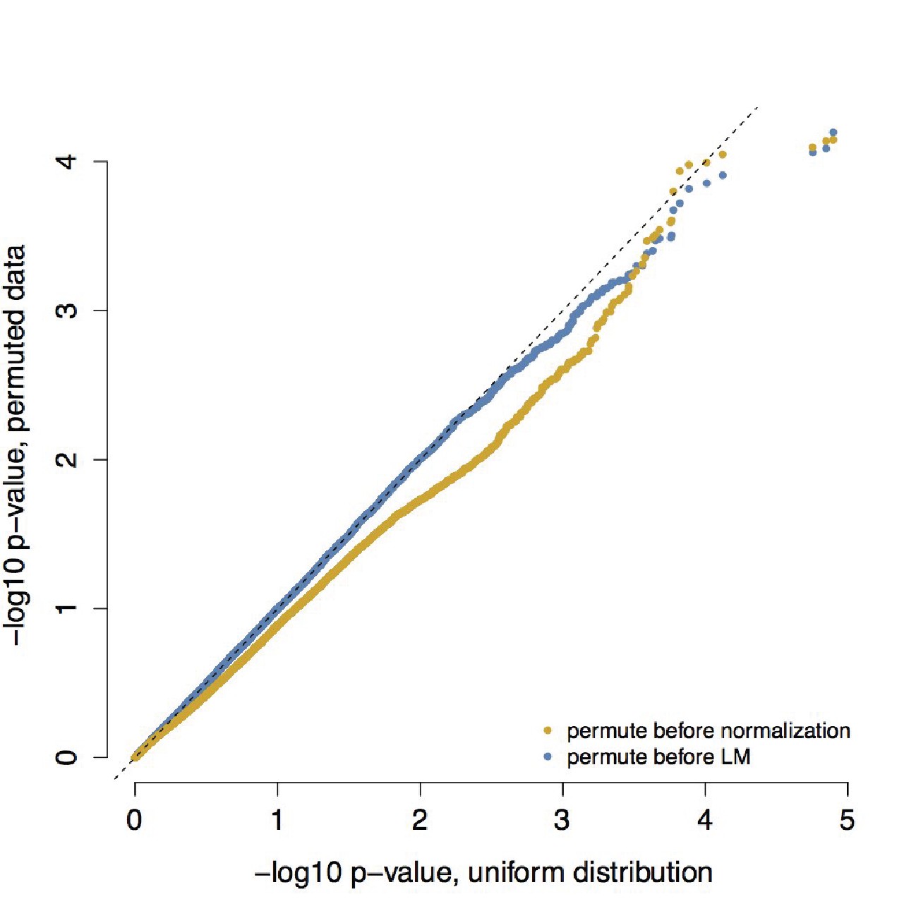
QQ-plot confirming that empirical null distributions approximate a uniform distribution.
To understand whether our analyses testing for differences in correlation between healthy individuals and those with metabolic syndrome produced biased p-value distributions, we confirmed that permuting individual health status (metabolic syndrome/healthy) produced the expected uniform p-value distribution. We performed permutations using two approaches: (i) we permuted health status prior to normalization, calculation of products, and linear mixed effects modeling and (ii) we permuted health status prior to linear mixed effects modeling alone. For each approach, we performed 10 independent permutations; p-values from these 10 permutations were combined and are plotted here together against a uniform distribution.
Figure 4 with 6 supplements
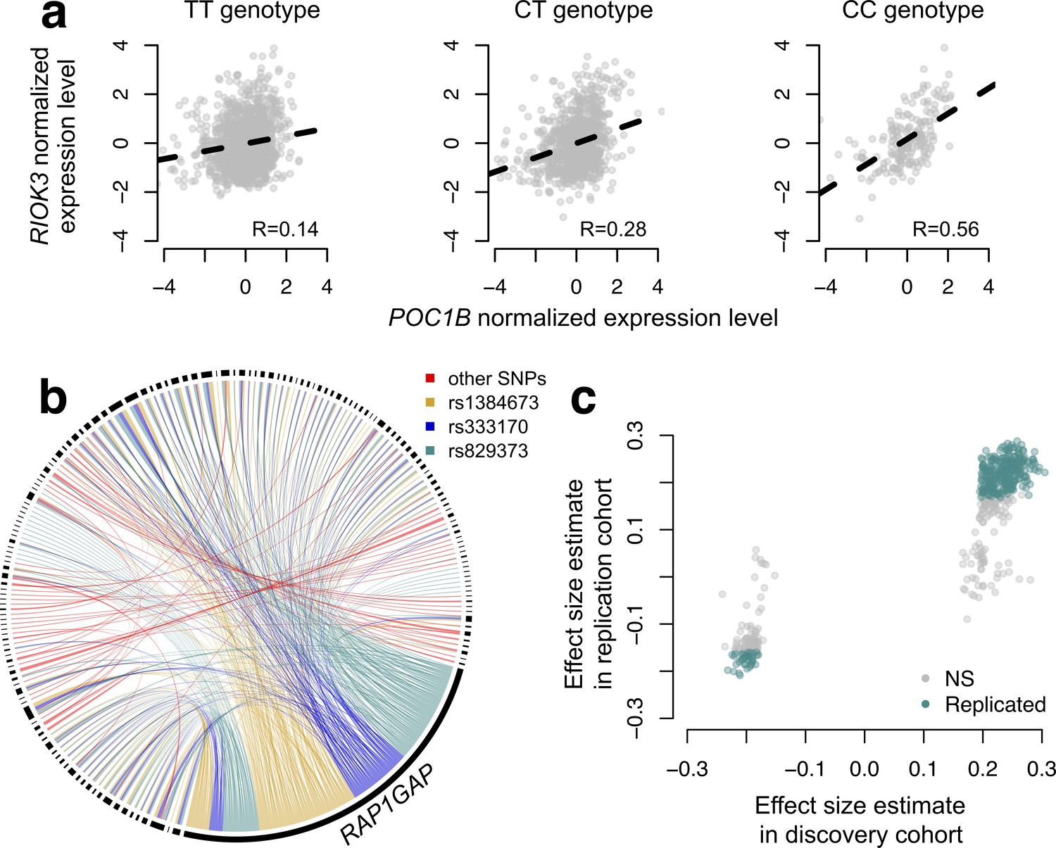
CILP approach reveals hundreds of correlation QTLs.
(a) Example of a correlation QTL, where the SNP rs10953329 controls the magnitude of the correlation between the mRNA expression levels of POC1B and RIOK3. (b) Gene pairs involved in significant (FDR < 10%) correlation QTL. Each black segment represents a gene, and each line connecting two segments represents a significant correlation QTL. Lines are colored by the identity of the SNP controlling the magnitude of the correlation between the gene pair. (c) Many correlation QTL identified in the NESDA discovery set (n = 2477) replicate in a second set of NESDA participants (n = 1337). Plot shows effect sizes for each correlation QTL, estimated in the discovery or replication cohort (effect sizes are derived from in matrixEQTL (Shabalin, 2012)). Points are colored to indicate whether a given correlation QTL passed Bonferroni correction in the replication dataset.
Figure 4—figure supplement 1
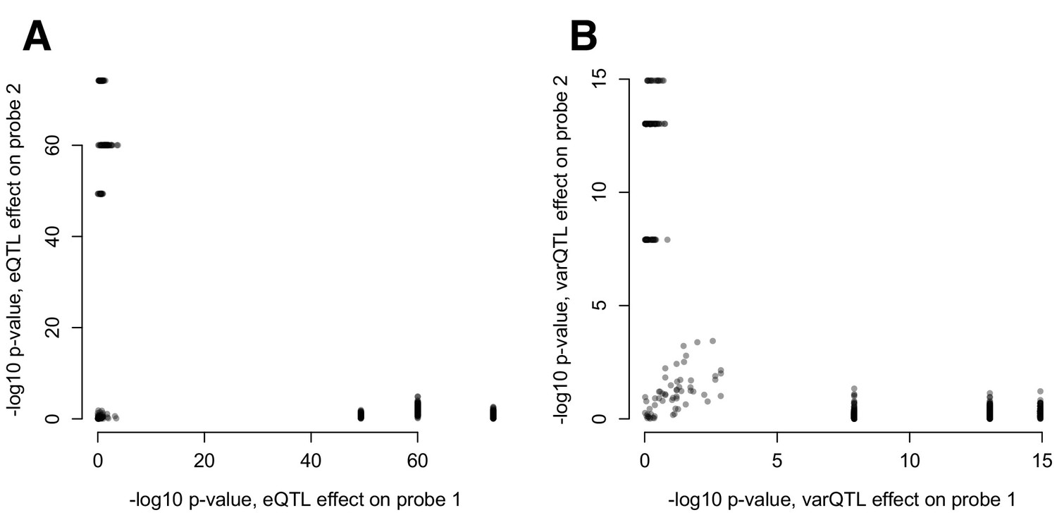
(A) Mean and (B) variance effects of SNPs identified as significant correlation QTL.
For each SNP that significantly affected the correlation between a pair of gene expression probes (n = 484 correlation QTL), we asked whether the SNP also affected the mean or variance of the expression levels of each probe. The 3 SNPs that show strong effects on the mean and variance of one co-expressed probe but not the other are all in cis with RAP1GAP (and affect the mean and variance of this gene; see also Figure 4—figure supplement 2).
Figure 4—figure supplement 2
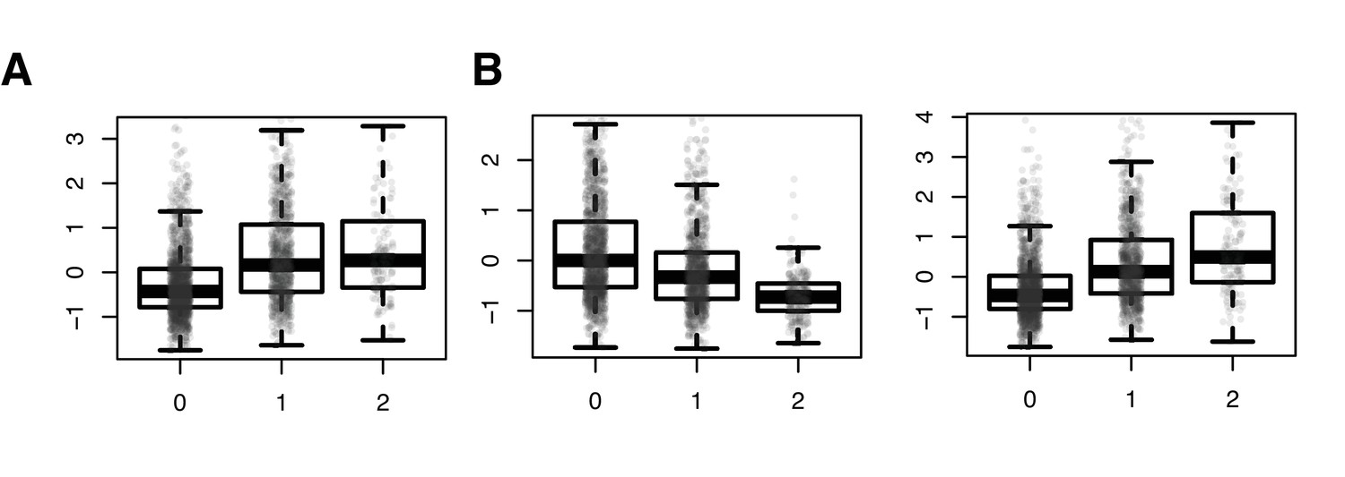
SNPs driving correlation QTL (between RAP1GAP and other many other genes) are also strong cis eQTL for RAP1GAP.
Results from a linear model predicting normalized RAP1GAP gene expression in the NESDA dataset as a function of SNP genotype, controlling for sex, age, smoking behavior, major depressive disorder, red blood cell counts, year of sample collection, study phase, and the first five principal components from a PCA on the filtered genotype call set: (A) rs829373: beta = 0.541, p<10−16; (B) rs333170: beta = −0.447, p<10−16; (C) rs1384673: beta = 0.591, p<10−16.
Figure 4—figure supplement 3
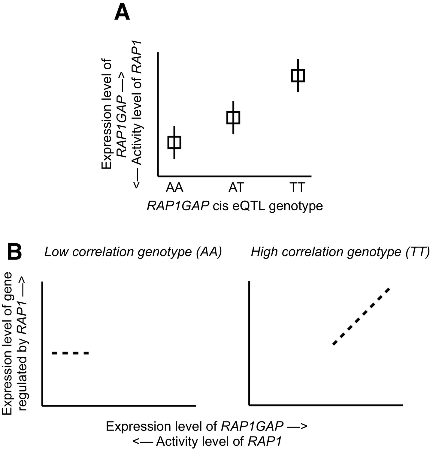
Mechanistic relationship between RAP1GAP eQTL and correlation QTL.
(A) Several SNPs driving correlation QTL between RAP1GAP and genes regulated by RAP1 are also strong eQTL for RAP1GAP (specifically, rs829373, rs333170, rs333170). The primary function of RAP1GAP is to convert the transcription factor RAP1 – a master regulator of T and B-cell activation, cell adhesion, and neuronal differentiation – from its active GTP-bound form to its inactive GDP-bound form. Thus, through strong eQTL near RAP1GAP, individuals are biased toward high RAP1GAP mRNA expression and low RAP1 activity (the TT genotype in this example) or toward low RAP1GAP mRNA expression and high RAP1 activity (the AA genotype in this example). In other words, within a given individual, RAP1 exists in its constitutively active or inactive form depending on the genetic variation the individual harbors near RAP1GAP. (B) Intra-genotypic variation in RAP1 activity levels is only meaningful for the low activity genotype (the TT genotype in this example). In contrast, for individuals with the high activity genotype (AA in this example), the targets of RAP1 are constitutively repressed in all individuals, and dialing up or dialing down RAP1 activity levels has little effect. Together, this pattern produces correlation QTL involving SNPs that are also strong cis eQTL for RAP1GAP.
Figure 4—figure supplement 4
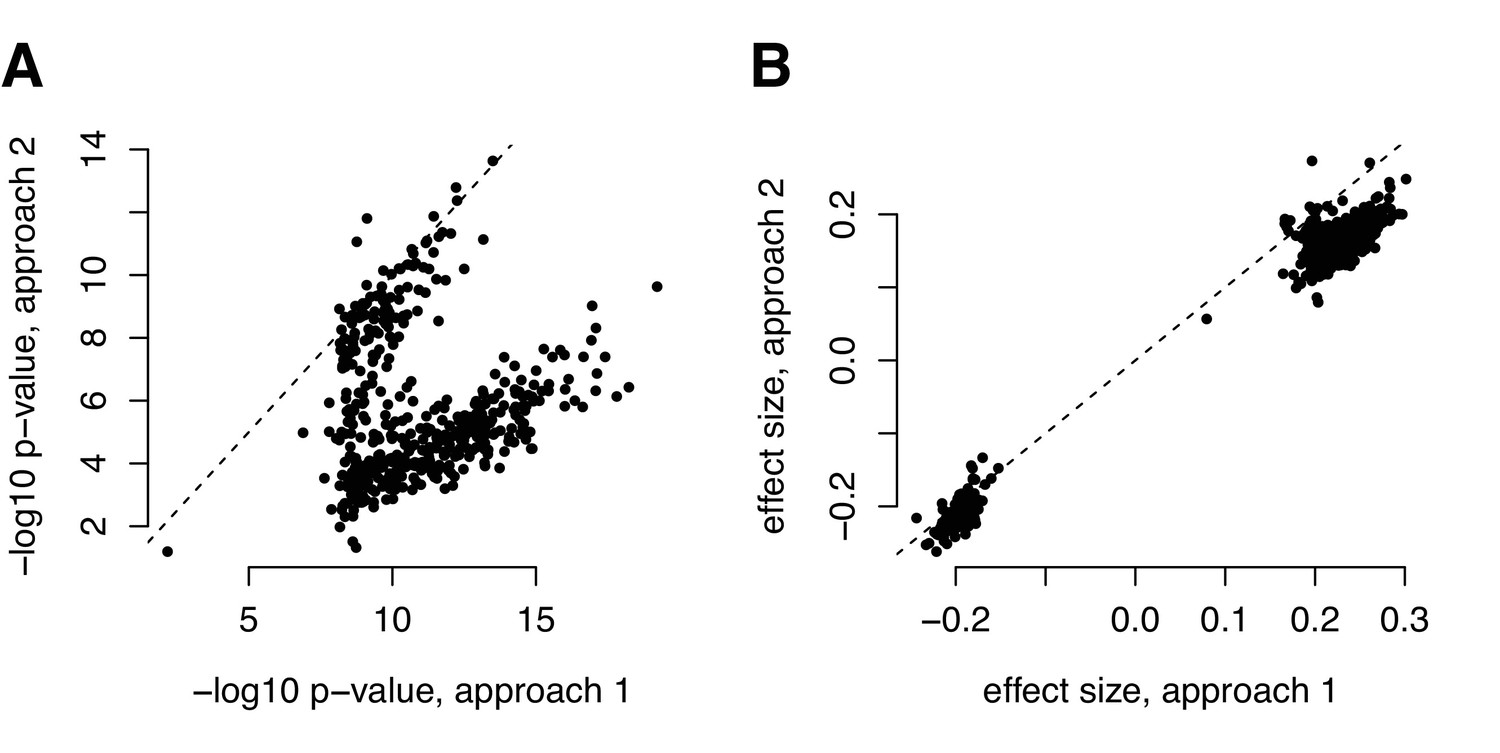
Comparison of (A) p-values and (B) effect size estimates from different approaches for identifying correlation QTL.
Our metabolite analyses focused on data that were z-score normalized within each health status group (metabolic syndrome versus healthy). The parallel of this approach for mapping correlation QTLs would be to z-score normalize each transcript within each genotypic class before computing the product between two focal transcripts (y-axis, labeled ‘approach 2’); however, this pipeline is infeasible for efficient genome-wide QTL mapping, as it would require us to recalculate the outcome variable for every association test we performed. For the correlation QTL analyses presented in the main text, we therefore normalized, mean centered, and scaled each transcript before any product calculation (x-axis, labeled ‘approach 1’). This approach is different than normalizing each transcript within each genotypic class, but attempts to circumvent the same set of potential issues and has the advantage of only needing to be performed once (making it much more computationally feasible for genome-wide screens). For comparison, we present the effects size estimates and p-values from the two approaches for the set of 484 significant correlation QTL we identified with approach 1.
Figure 4—figure supplement 5
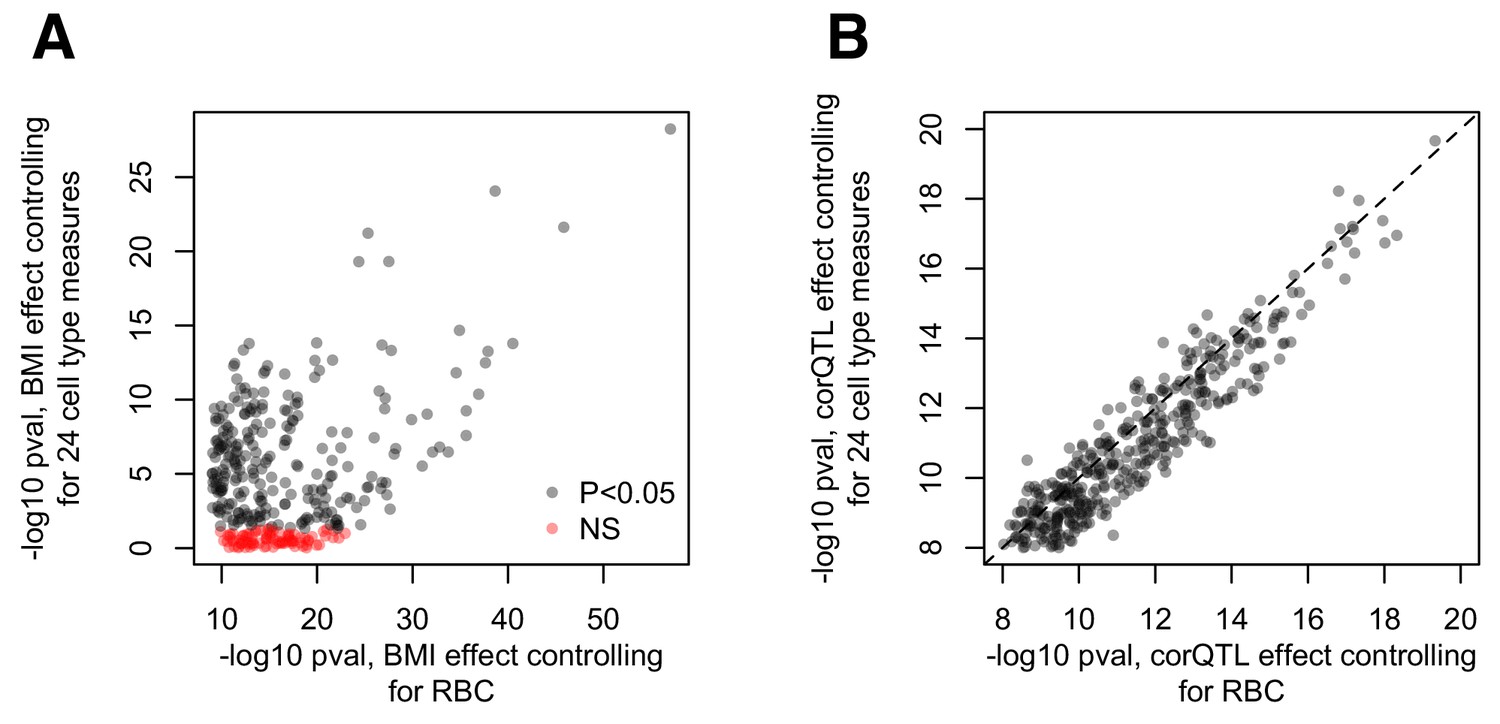
Cell type effects on (A) BMI-gene expression correlations and (B) estimations of the correlation QTL effect.
(A) Comparison of the -log10 p-values for the effect of BMI estimated using the pipeline presented in the main text (x-axis) versus a parallel analysis where 24 measures of cell type heterogeneity are included as covariates (y-axis). The pipeline presented in the main text included red blood cell counts as a covariate, but no other measures of cell type heterogeneity. The alternative pipeline includes this measure as well as 23 additional measures inferred through PCA or deconvolution (Newman et al., 2015; Preininger et al., 2013). (B) Comparison of the -log10 p-values for the correlation QTL effect, obtained from the pipeline described in the main text (x-axis) versus a pipeline that regressed out 24 measures of cell type heterogeneity from the gene expression data before correlation QTL testing (Pearson correlation, cor = 0.937, p<10−16).
Figure 4—figure supplement 6
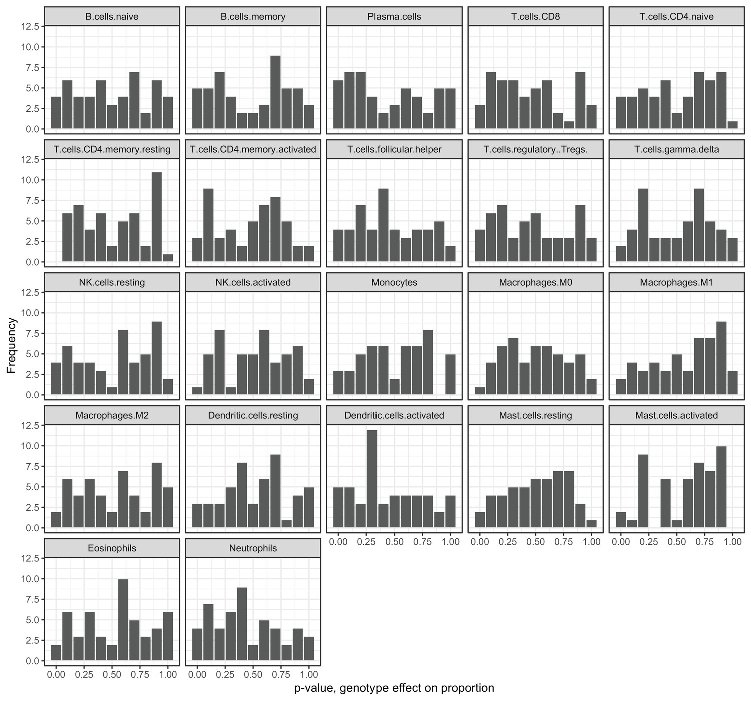
Genotypes at correlation QTLs do not predict cell type heterogeneity.
Each plot represents the p-value distribution obtained from testing whether genotype at each unique correlation QTL SNP influences cell type proportion estimates. Results are shown for the 22 cell type measures inferred through deconvolution in CIBERSORT (Newman et al., 2015).
Tables
Table 1
Power to detect simulated correlation QTL across a wide range of scenarios (n = 1000 for all simulations).
https://doi.org/10.7554/eLife.40538.005| Simulation parameters | ||||||||
|---|---|---|---|---|---|---|---|---|
| (1) Correlation QTL effect* | x | x | x | x | x | x | x | x |
| (2) Genotype predicts the mean of gene one expression levels† (e.g., through an eQTL or proportion QTL) | x | x | x | |||||
| (3) Genotype predicts the mean of gene two expression levels† | x | |||||||
| (4) Genotype predicts the variance of gene one expression levels‡ (e.g., through a varQTL) | x | x | ||||||
| (5) A variable that is random with respect to genotype predicts the mean of gene one expression levels†(e.g., through technical, environmental, or cell type heterogeneity effects) | x | |||||||
| (6) A variable that is random with respect to genotype predicts the mean of gene two expression levels† | x | |||||||
| (7) A variable that is random with respect to genotype predicts the variance of gene one expression levels‡(e.g., through technical, environmental, or cell type heterogeneity effects) | x | x | ||||||
| (8) A variable that is random with respect to genotype predicts the variance of gene two expression levels‡ | x | |||||||
| Results | ||||||||
| Power (proportion of true positives detected, Bonferroni-corrected p<0.05) | 0.5091 | 0.4934 | 0.5055 | 0.0716 | 0.0679 | 0.4998 | 0.0884 | 0.0533 |
| False positive rate (proportion of true negatives detected, nominal p<0.05) | 0.0519 | 0.0529 | 0.0494 | 0.0532 | 0.0507 | 0.0527 | 0.0529 | 0.0522 |
-
Simulated effect sizes were as follows: correlation QTL* = 0.3, mean effects† = 1, variance effects ‡ = 10. When Bonferroni-corrected p-values were used, the false positive rate was 0 across all simulation scenarios. Abbreviations: eQTL = expression QTL and vQTL = variance QTL.
Additional files
-
Supplementary file 1
Power to detect simulated correlation QTL using a modified version of CILP (n = 1000 for all simulations).
- https://doi.org/10.7554/eLife.40538.017
-
Supplementary file 2
List of analyzed metabolites and functional annotations (following Nath et al., 2017).
- https://doi.org/10.7554/eLife.40538.018
-
Supplementary file 3
Enrichment of metabolite functional annotations among significantly differentially correlated pairs.
- https://doi.org/10.7554/eLife.40538.019
-
Supplementary file 4
Significant correlation QTL in NESDA.
- https://doi.org/10.7554/eLife.40538.020
-
Supplementary file 5
Location of correlation QTL SNPs in relation to gene expression probes.
- https://doi.org/10.7554/eLife.40538.021
-
Supplementary file 6
Enrichment of gene ontology categories among genes involved in significant correlation QTL.
- https://doi.org/10.7554/eLife.40538.022
-
Supplementary file 7
Individuals classified as healthy or having metabolic syndrome based on a random forests classifier.
- https://doi.org/10.7554/eLife.40538.023
-
Supplementary file 8
Effects of cell type heterogeneity on BMI.
- https://doi.org/10.7554/eLife.40538.024
-
Supplementary file 9
Effects of genotype on cell type heterogeneity.
- https://doi.org/10.7554/eLife.40538.025
Download links
A two-part list of links to download the article, or parts of the article, in various formats.
Downloads (link to download the article as PDF)
Open citations (links to open the citations from this article in various online reference manager services)
Cite this article (links to download the citations from this article in formats compatible with various reference manager tools)
Genetic and environmental perturbations lead to regulatory decoherence
eLife 8:e40538.
https://doi.org/10.7554/eLife.40538


