The origins and relatedness structure of mixed infections vary with local prevalence of P. falciparum malaria
- University of Oxford, United Kingdom
- Wellcome Sanger Institute, United Kingdom
Figures
Figure 1 with 2 supplements
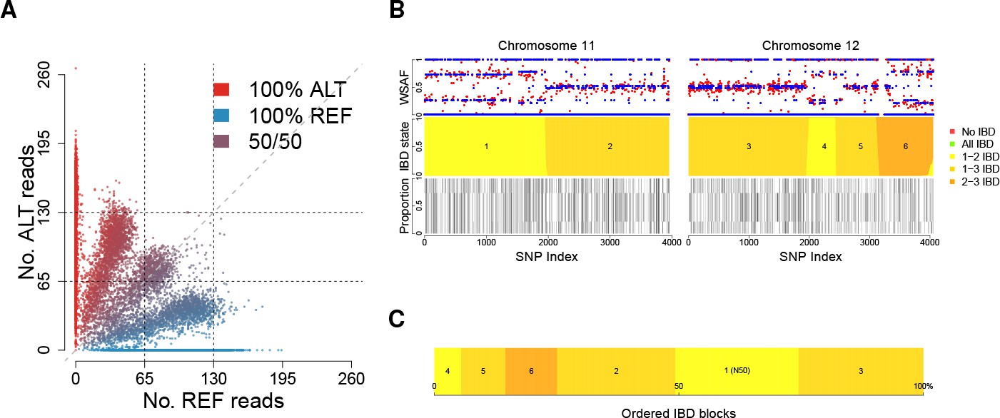
Deconvolution of a complex field sample PD0577-C from Thailand.
(A) Scatter-plot showing the number of reads supporting the reference (REF: x-axis) and alternative (ALT: y-axis) alleles. The multiple clusters indicate the presence of multiple strains, but cannot distinguish the exact number or proportions. (B) The profile of within-sample allele frequency along chromosomes 11 and 12 (red points) suggests a changing profile of IBD with three distinct strains, estimated to be with proportions of 22%, 52% and 26% respectively (other chromosomes omitted for clarity, see Figure 1—figure supplement 1); blue points indicate expected allele frequencies within the isolate. However, the strains are inferred to be siblings of each other: green segments indicate where all three strains are IBD (Note: green segments do not appear in this example, but occur in Figure 5); yellow, orange and dark orange segments indicate the regions where one pair of strains are IBD but the others are not. In no region are all three strains inferred to be distinct. (C) Statistics of IBD tract length, in particular illustrating the N50 segment length. A graphical description of the modules and workflows for DEploidIBD is given in Figure 1—figure supplement 2.
Figure 1—figure supplement 1

Whole genome deconvolution of field sample PD0577-C.
The outer ring shows the expected within-sample allele frequency (WSAF) (blue) and observed WSAF (red) across the genome. Red and blue points indicate observed and expected allele frequencies within the isolate. The inner ring indicates the IBD states among the three strains: green segments indicate where all three strains are IBD; yellow, orange and dark orange segments indicate the regions where one pair of strains are IBD but the others are not. In no region are all three strains inferred to be distinct, suggesting that the three strains are siblings.
Figure 1—figure supplement 2
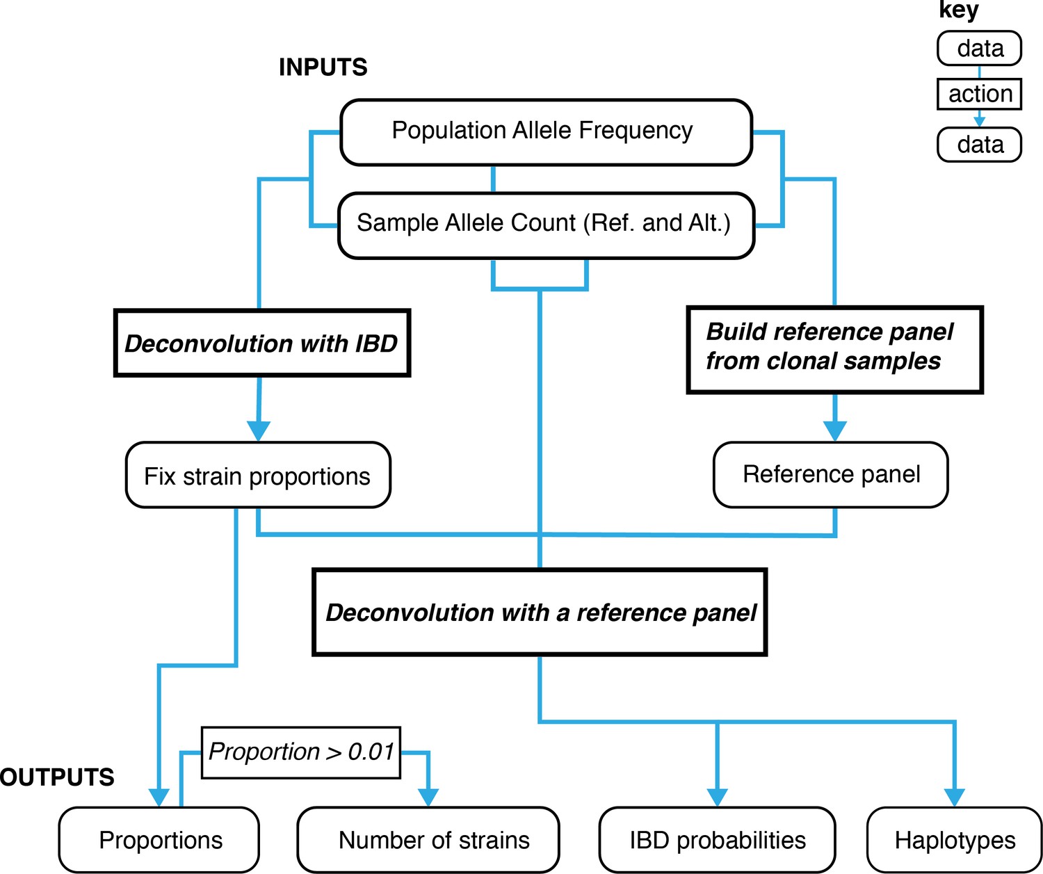
A graphical overview of the data types and work flows for DEploidIBD.
The boxes at the bottom represent final outputs of the pipeline. The rectangular boxes indicate when DEploidIBD is executed, with inputs highlighted by blue arrows. The process has three key steps: Step 1. A reference panel for the set of samples is constructed from high confidence clonal haplotypes, either identified from within a study or from an external resource, such as Pf3k. Step 2: DEploidIBD, using population level allele frequencies, is used to infer the number of strains, strain proportions and IBD profile within each sample. Step 3: DEploidIBD is re-run on each sample to infer haplotypes, but with the proportions estimated in Step two fixed and this time using the haplotype (LD-aware) method previously implemented in DEploid.
Figure 2 with 5 supplements
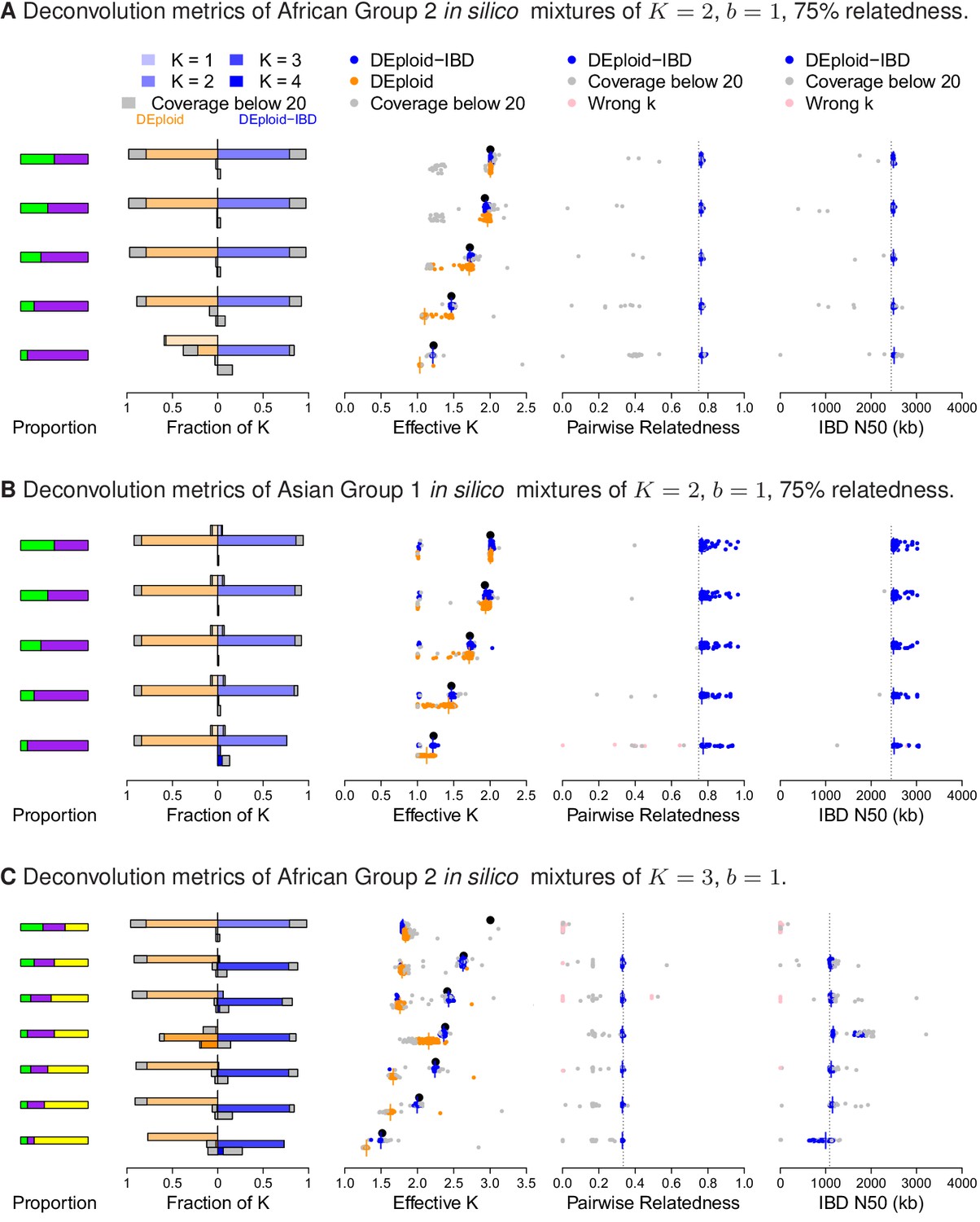
Performance of DEploidIBD and DEploid on 100 in silico mixtures for each of three different scenarios.
From the left to the right, the panels show the strain proportion compositions, distribution of inferred in a vertically-oriented histogram (top: , bottom: ), using both methods: DEploid in orange and DEploidIBD in blue, effective number of strains, pairwise relatedness and IBD N50 (the latter two only for DEploidIBD). From top to the bottom, cases are ordered from even strain proportions to the most imbalanced composition. Grey points identify experiments of low coverage data (median sequencing depth < 20), and pink identify cases where is inferred incorrectly. (A) In silico mixtures of two African strains with high-relatedness (75%) for 7757 (s.d. 178) sites on Chromosome 14, Note that DEploid underestimates the minor strain proportion if strains have high relatedness. In the extreme case, DEploid misclassifies a -mixture as clonal, whereas DEploidIBD consistently estimates the correct proportions. (B) In silico mixtures of two Asian strains with high-relatedness (75%) for 3041 sites (s.d. 227) on Chromosome 14, Note that DEploid underestimates strain number when the minor strain is low frequency, while DEploidIBD typically performs well. (C) In silico mixtures of three African strains, where each pair is IBD over a distinct third of the chromosome. Note that both methods fail to deconvolute the case of equal proportions. However, for unbalanced mixtures, DEploidIBD consistently performs better than DEploid.
Figure 2—figure supplement 1
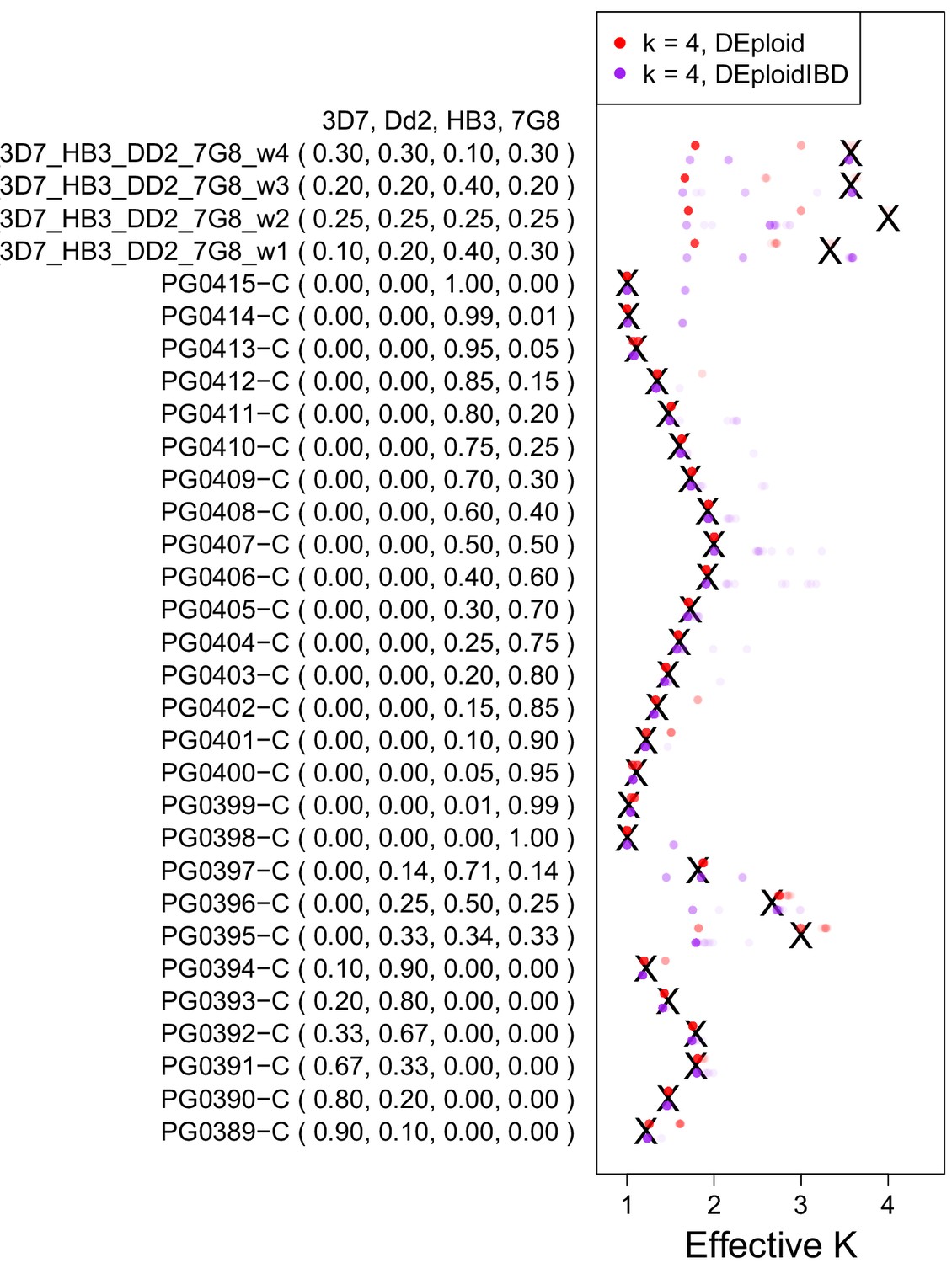
Validation of DEploidIBD using 27 in vitro lab mixtures and four in silico mixtures.
A reference panel of the laboratory strains (3D7, Dd2, HB3 and 7G8; Panel V) was used to deconvolute samples with DEploid. Each experiment is performed with and without IBD inference and with the maximum number of 4 strains. Black crosses indicate the true effective number of strains. Coloured crosses (DEploid in red, DEploidIBD in purple) indicate median values obtained from 30 replicates using the algorithm indicated in the legend. The coloured dots show the inferred effective number of strains across replicates with intensity proportional to fraction. Note one sample where balanced proportions of three strains results in the LD-free (DEploid-IBD) approach fitting the data as a mixture of two strains with proportions of 1/3 and 2/3. For in silico mixtures of four strains, DEploid performs poorly. DEploidIBD shows some improvement in unbalanced mixtures, though misclassifies mixtures as only having three strains.
Figure 2—figure supplement 2
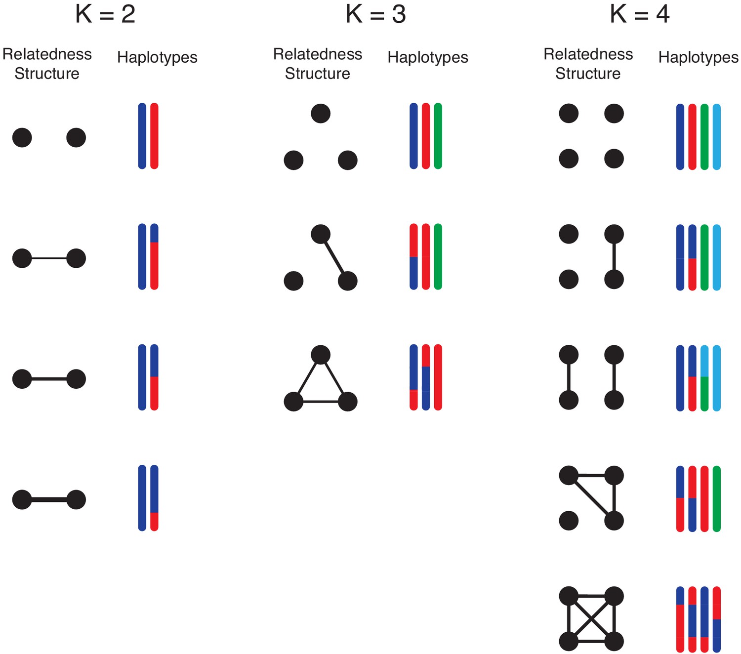
Illustration of simulation study design.
We conduct simulation studies to mimic -mixtures (top row) as results of -biting events, where and . For each -mixture, the left column illustrate the overall relationship between strains (black dots): connected dots imply strains are from the same mosquito bite. The level of relatedness between parasite strains is reflected by the haplotype segment copied from the parental strains within the mosquito. Each colour represents a unique strain within the mosquito, which we randomly draw from field clonal haplotypes. For example, when , we consider the case that the two strains are from two independent mosquito bites; on the other hand, when two strains are from the same mosquito bite, we consider scenarios of low (25%), moderate (50%) and high (75%) relatedness between two sibling strains. These events are represented in the second, third and forth rows respectively. For , we consider mixed-infection events as products of three mosquito bites, two mosquito bites and a single bite. For , we consider mixed infections as products of four mosquito bites, three mosquito bites, two mosquito bites and a single bite. We further divide the possibilities of the 2-bite event into the case that both bites pass on two strains (2 + 2) and the other possibility that one bite passes on a single strain and the other bit passes on three strains (1 + 3).
Figure 2—figure supplement 3
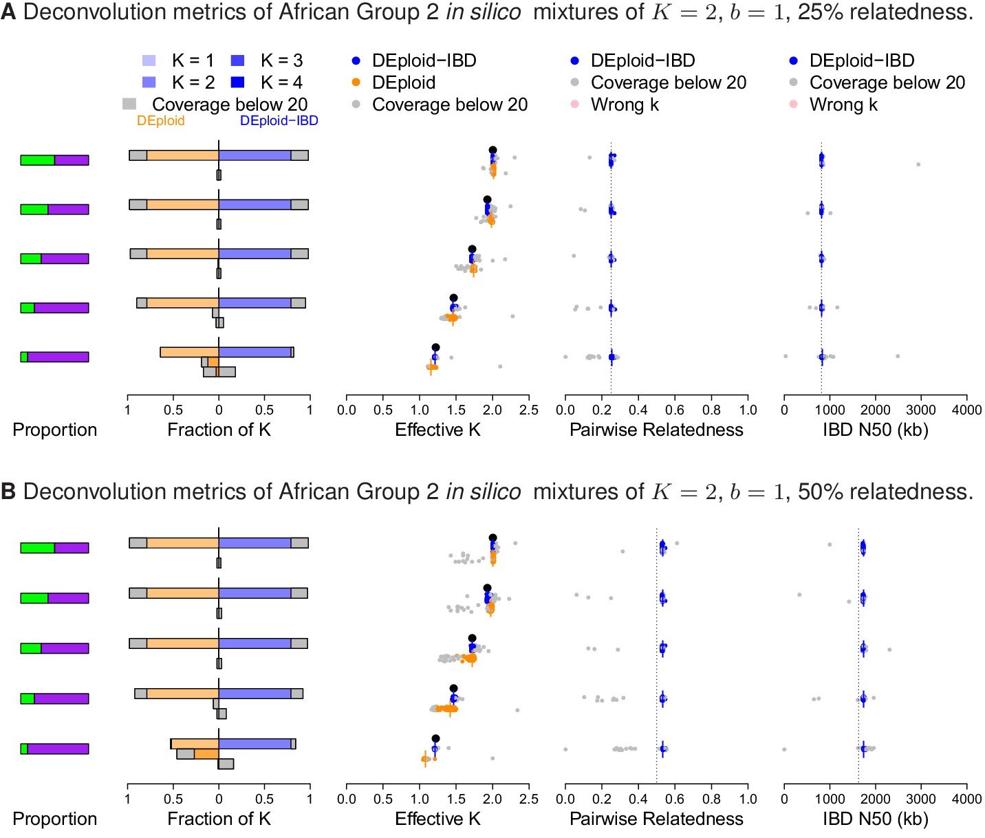
Additional comparison of DEploidIBD and DEploid on 100 in silico mixtures of two strains from Africa with low and moderate relatedness, illustrated by sub panels (A) and (B), respectively.
Detailed panel description can be found in the caption to Figure 2. DEploid generally performs well for samples of low within sample relatedness, though struggles when the minor strain proportion is below 30%. In contrast, DEploidIBD consitently performs well.
Figure 2—figure supplement 4
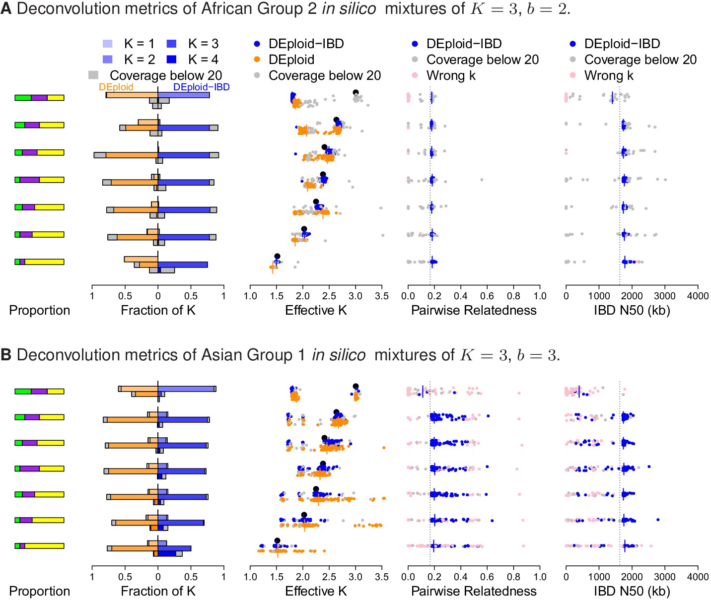
Additional comparison of DEploidIBD and DEploid on in silico bite mixtures of strains from Africa and Asia, illustrated by sub panels (A) and (B), respectively.
Detailed panel descriptions can be found in the caption to Figure 2. The unrelated strain provides a strong signal in allele frequency imbalance for DEploid to detect and therefore performs better than dealing with mixtures. Comparing (A) and (B), pairwise relatedness estimates are noisy in Asia because of the background IBD. However, background relatedness generates shorts segments of IBD and therefore leads to IBD N50 underestimation.
Figure 2—figure supplement 5
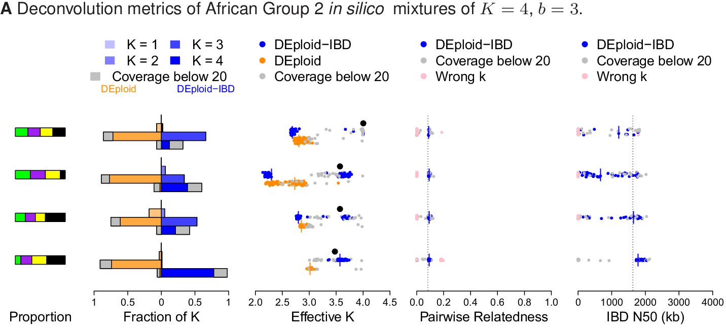
Comparison of DEploidIBD and DEploid on 100 in silico bite mixtures of four strains from Africa.
Detailed panel descriptions can be found in the caption to Figure 2. DEploid performs poorly in all cases. In contrast, DEploidIBD performs well when all four strains have unequal proportions, but is less accurate when some strains have equal proportion.
Figure 3
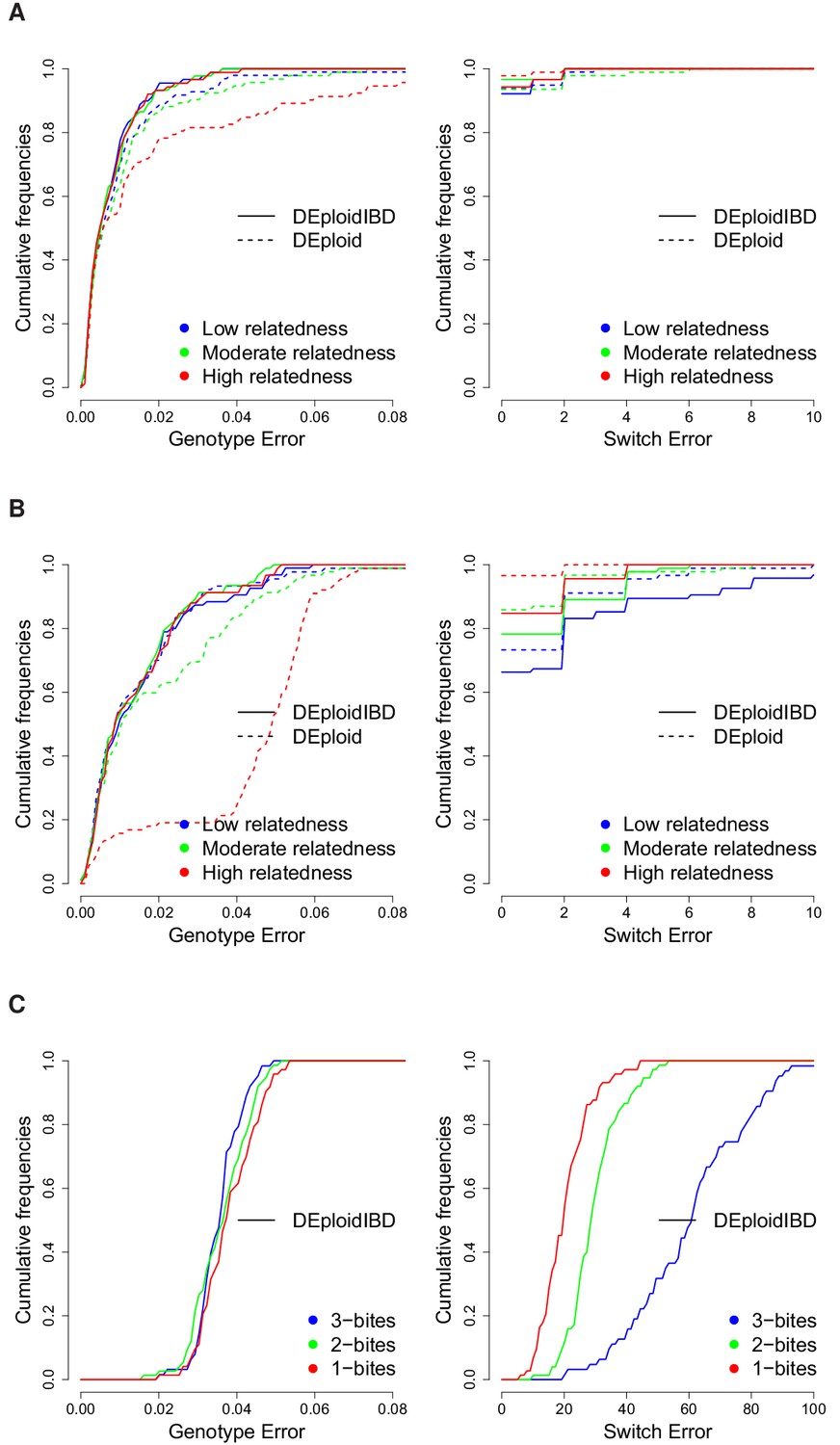
Cumulative distribution of the average per site genotype error (left) and switch error (right) across simulated mixtures (measured at sites that are heterozygous in the sample or sample-specific reference panel).
(A) Error rates of Asian in silico samples of three levels of IBD (25%, 50% and 75%) for a mixture with proportions of 20/80%. Because DEploidIBD estimates proportions more accurately, it enables better haplotype inference. (B) Error rates of African in silico samples of three levels of IBD (25%, 50% and 75%) for a mixture with proportions of 20/80%. Inference in Asia benefits from better reference panels (due to lower overall diversity) and therefore gives lower error rates than in Africa. (C) DEploidIBD error rates for African in silico samples of three mosquito biting scenarios for a mixture with proportions of 10/10/80%. The additional strain increases the difficulty of haplotype inference, particularly in the case of three independent bites.
Figure 4
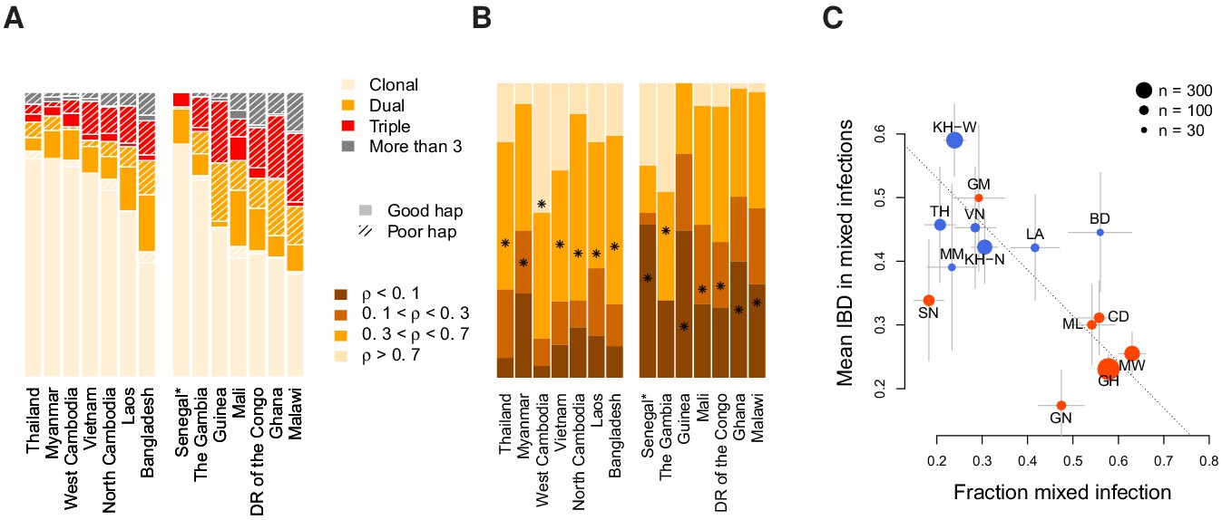
Characterisation of mixed infections across 2344 field samples of Plasmodium falciparum.
(A) The fraction of samples, by population, inferred by DEploidIBD to be (clonal), (dual), (triple), or (More than 3). Populations are ordered by rate of mixed infections within each continent. We use shaded regions to indicate the distribution of 787 samples that have low-confidence deconvoluted haplotypes. Senegal is marked with an asterisks as these samples were screened to be clonal. (B) The distribution of average pairwise IBD sharing within mixed infections (including dual, triple and quad infections), broken down into unrelated (where the fraction of the genome inferred to be IBD, , is ), low IBD (, sib-level () and high (). Stars indicate the average IBD scaled between 0 and 1 from bottom to the top. Populations follow the same order as in Panel A. (C) The relationship between the rate of mixed infection and level of IBD. Populations are coloured by continent, with size reflecting sample size and error bars showing ±1 s.e.m.. The dotted line shows the slope of the regression from a linear model. Abbreviations: SN-Senegal, GM-The Gambia, NG-Nigeria, GN-Guinea, CD-The Democratic Republic of Congo, ML-Mali, GH-Ghana, MW-Malawi, MM-Myanmar, TH-Thailand, VN-Vietnam, KH-Cambodia, LA-Laos, BD-Bangladesh.
Figure 5
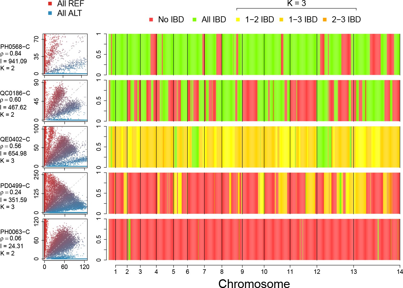
Example IBD profiles in mixed infections.
Plots showing the ALT versus REF plots (left hand side) and inferred IBD profiles along the genome for five strains of differing composition. From top to bottom: A dual infection of highly related strains (); a dual infection of two sibling strains (); a triple infection of three sibling strains (note the absence of stretches without IBD); a triple infection of two related strains and one unrelated strain; and a triple infection of three unrelated strains. The numbers below the sample IDs indicate the average pairwise IBD, , the mean length of IBD segments, , in kb and the inferred number of distinct strains, , respectively.
Figure 6
Identifying sibling strains within mixed infections.
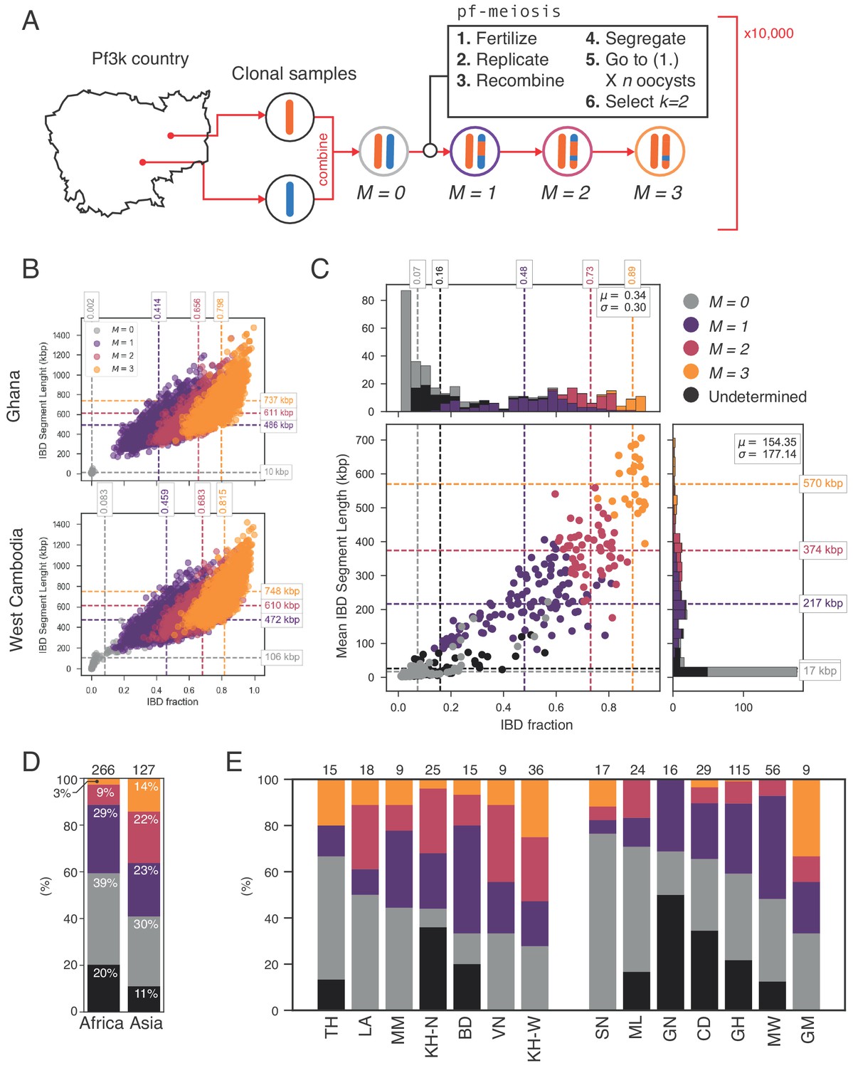
(A) Schematic showing how IBD fraction and IBD segment length distributions are created for mixed infections using pf-meiosis. Two clonal samples from a given country are combined to create an unrelated (, where is number of meioses that have occurred) mixed infection. The infection is then passed through 3 rounds of pf-meioses to generate classes, representing serial transmission of the mixed infection ( are siblings). (B) Simulated IBD distributions for for Ghana (top) and West Cambodia (bottom). A total of 10,000 mixed infections are simulated for each class, from 500 random pairs of clonal samples. (C) Classification results for 393 mixed infections from 13 countries. Undetermined indicates mixed infections with IBD statistics that were never observed in simulation. (D) Breakdown of class percentage by continent. Total number of samples is given above bars. Colours as in panel C (, grey; , purple; , pink; , orange; Undetermined, black). (E) Same as (D), but by country. Abbreviations as in Figure 4.
Figure 7
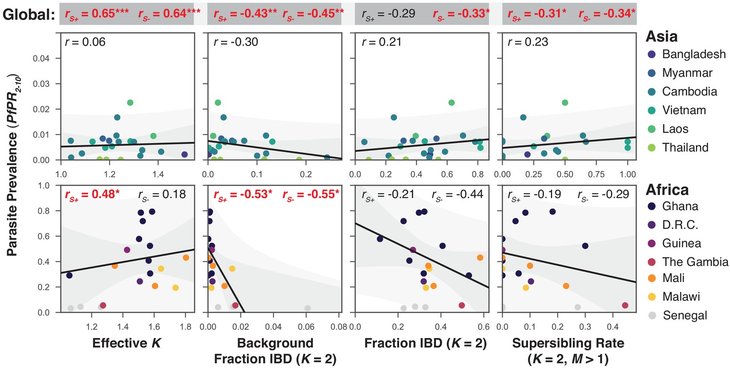
The relationship between P. falciparum prevalence and characteristics of mixed infection.
Four mixed infection statistics are shown including the average effective number of strains (Effective K, first column), given by , where is the proportion of the th strain; background IBD observed between clonal samples (Background Fraction IBD, second column); fraction IBD within mixed infections (Fraction IBD, third column); and the rate of mixed infections classified as having (Supersibling Rate, fourth column). Each point relates to a row in Table 1 from different sampling locations and years. Pearson’s is computed globally (shown at top in a grey box for each statistic), across Asian countries (upper panel) and across African countries (lower panel). Globally and for Africa, the correlations were computed including Senegal () and excluding Senegal (). The slope and confidence intervals for the regression line excluding Senegal are drawn. Significant correlations () are highlighted in red and significance levels indicated by asterisks (* , ** , *** ).
Appendix 1—figure 1
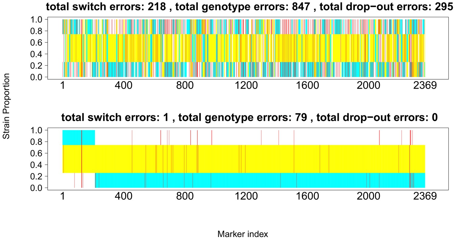
Comparison of true and inferred haplotypes for Chromosome 14 (2,369 SNPs) in the lab strain mixture sample PG0396-C after running DEploidIBD to infer strain number and proportions (top) and after subsequent refinement of haplotypes by running DEploid with Reference Panel V (bottom).
The yellow, cyan and white backgrounds identify the haplotype segments from strains 7G8, HB3 and Dd2 respectively. Numbers in the titles indicate the inferred switch, mismatch and dropout errors identified by the dynamic programming approach, with the cost of switch errors being twice that of other errors.
Appendix 2—figure 1

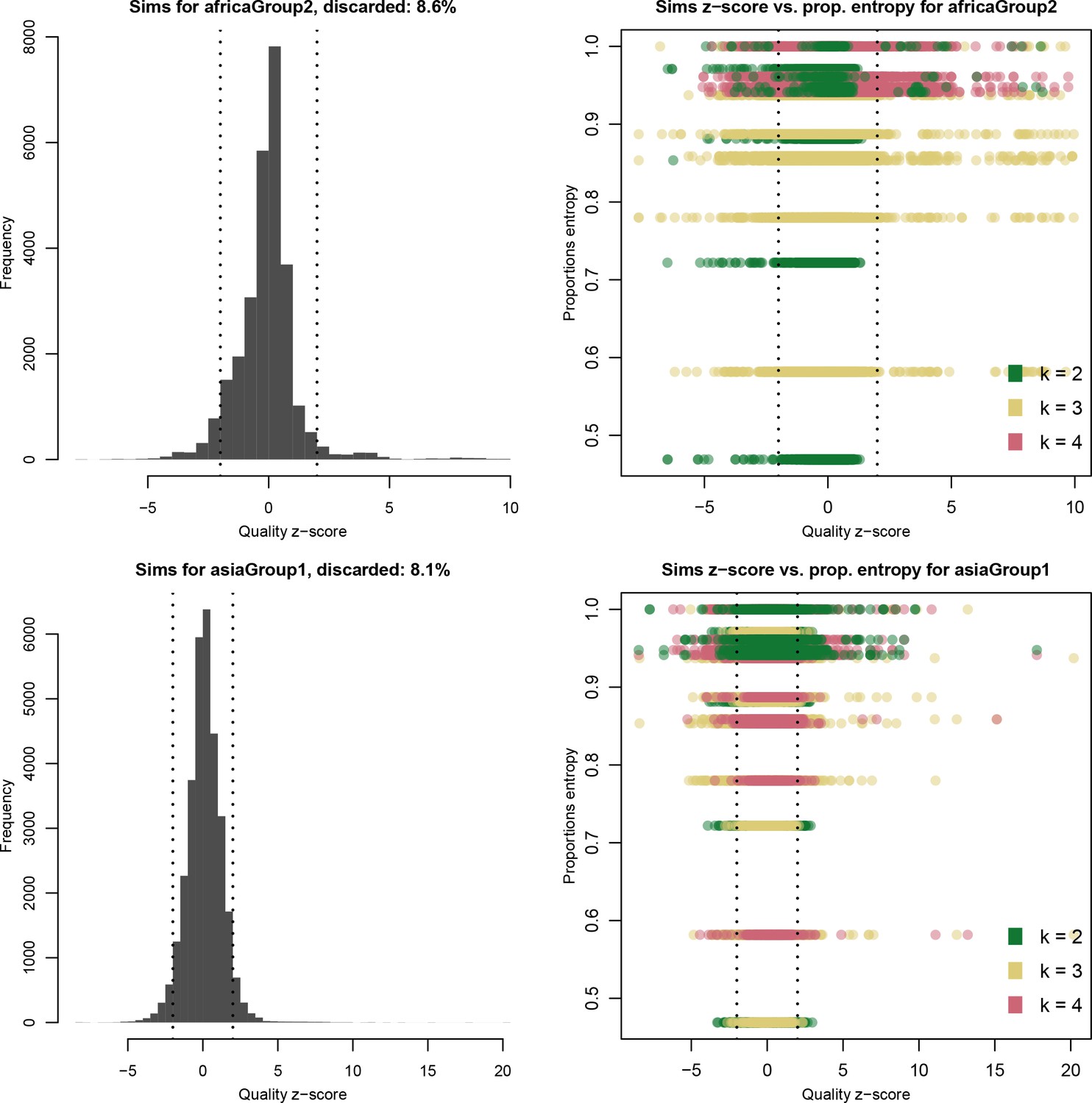
Distribution of quality scores haplotypes deconvolved from in silico mixtures using DEploid.
Each row represents a different population (Africa and Asia). The left panels represent the overall distribution of z-scores whereas the right panels stratify results according to the entropy of mixture proportions (y-axis) and number of strains (color).
Appendix 2—figure 2
Distribution of quality scores haplotypes deconvolved from in silico mixtures using DEploidIBD.
Each row represents a different population (Africa and Asia). The left panels represent the overall distribution of Z-scores whereas the right panels stratify results according to the entropy of mixture proportions (y-axis) and number of strains (color).
Appendix 3—figure 1
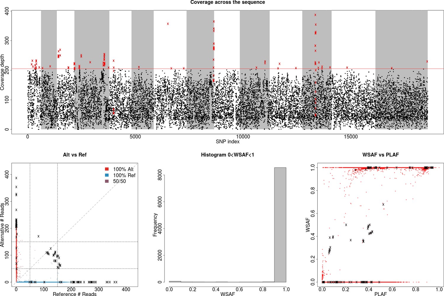
Identification of high leverage data points for filtering.
(Top) Plot showing total allele counts across all markers for field isolate PG0415. We observe a small number of heterozygous sites with high coverage (shown as crosses on the bottom-left plot), which can potentially mislead our model to over-fit the data with additional strains (above the dotted line). We used a threshold of ≥99.5% coverage to identify markers with high allele counts. Red crosses indicate markers that are filtered out. (Bottom-left) Scatter plot showing alternative against reference allele count. The marked black crosses refer to the outliers identified on the previous plot, which will cause the inference method to mistakenly identify the sample as being a mixed infection. (Bottom-middle) Histogram of allele frequency within sample. (Bottom-right) Allele frequency within sample (WSAF), compared against the population average (PLAF).
Appendix 3—figure 2
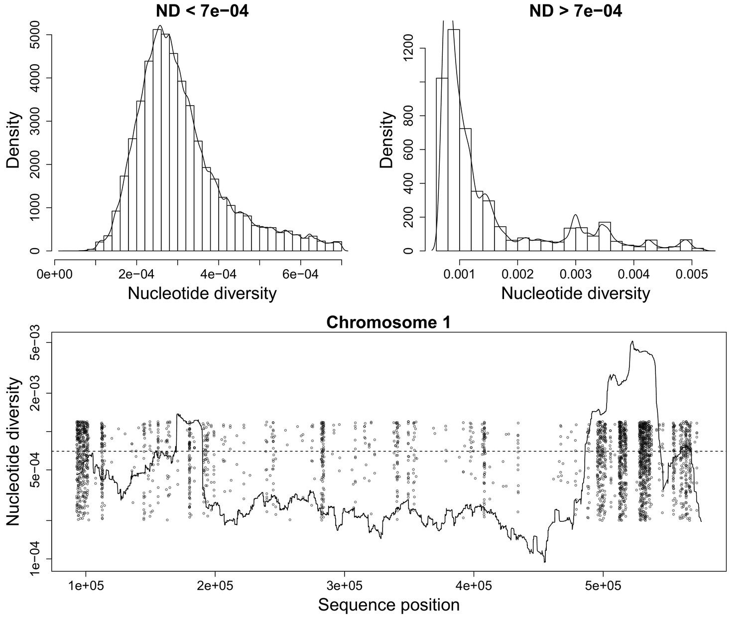
Nucleotide diversity for a sliding window size of 20,000 base pairs.
(Top) Histograms showing the heavy tail of ND beyond 0.0007. (Bottom) Figure showing ND along P. falciparum chromosome 1. Scattered Points mark chromosome positions of poorly genotyped SNPs which we exclude from the deconvolution process. These points are jitterred to ease visualization.
Appendix 3—figure 3
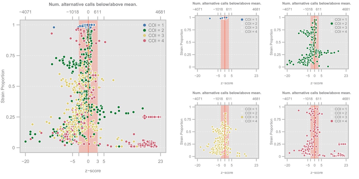
Diagnostic plots showing the distribution of haplotype quality (-scores) for the Ghanian samples.
Left. Scatterplot showing the relationship between haplotype -score and strain proportion. The top axis shows the number of alternative calls below/above the mean of the subset of clonal samples that correspond to a given -score. The vertical red line denotes a -score of whereas the red-shaded area indicate the haplotypes we retain Point colors show the COI level of the sample. Right. Four views of the same plot in which the samples have been highlighted according to their COI level.
Appendix 3—figure 4
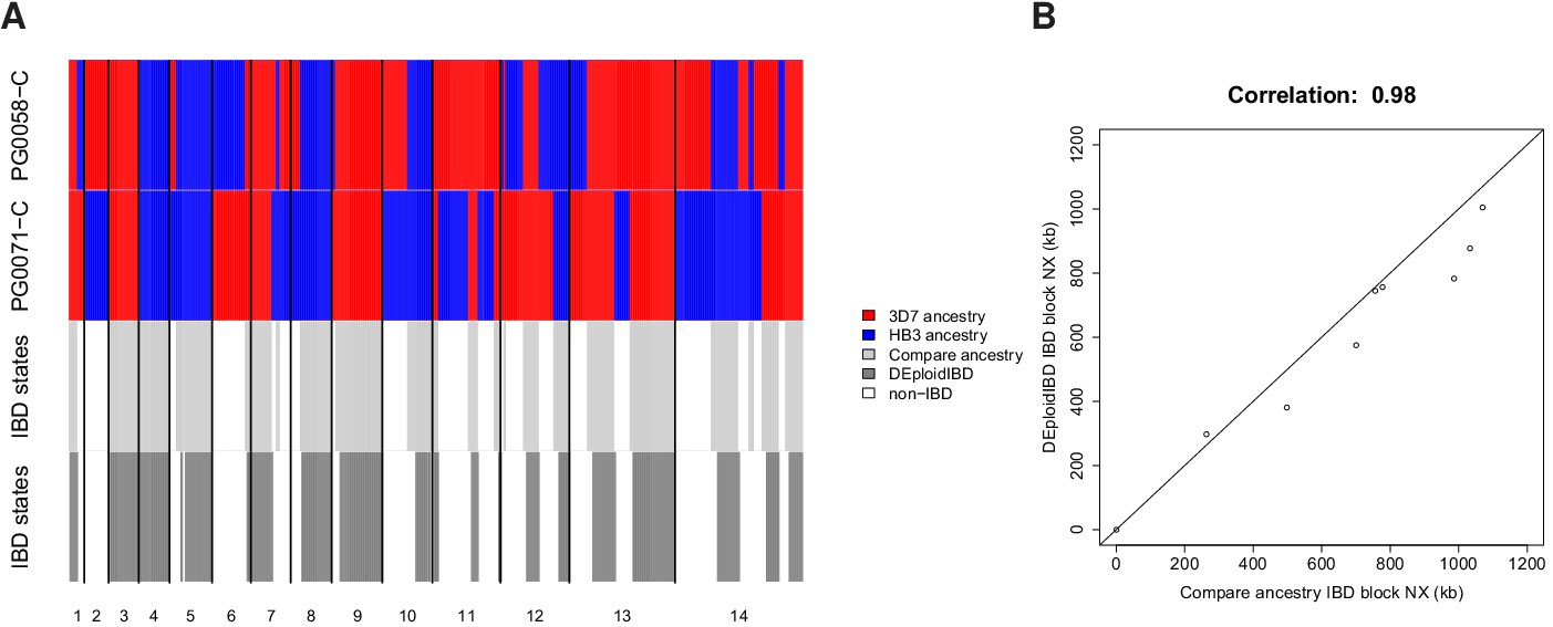
In silico validation of IBD estimation using lab crosses.
(A) Visual summary of of IBD block detection between DEploidIBD (top) and ancestral state inference from Li and Stephens (2003) (bottom), using artificial mixtures of lab crosses PG0071-C and PG0058-C (last tract). (B) Scatter plot of IBD segment Nx values extracted by comparing clonal sample ancestry (using DEploidIBD) on artificial mixtures.
Appendix 4—figure 1
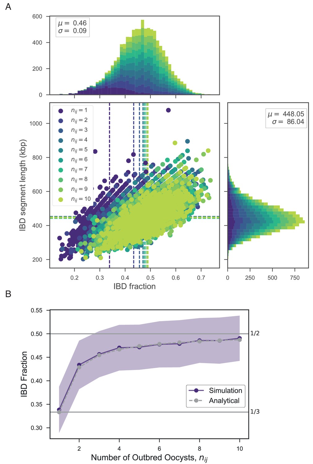
Exploring the relationship between number of outbred oocysts () and IBD.
(A) Joint IBD fraction and IBD segment length distributions for mixed infections simulated from two unrelated strains and a fixed number of outbred oocysts , using pf-meiosis. Mean values for each distribution are indicated by same-color dashed lines. Each distribution is created from 1000 simulated mixed infections. (B) Validation of theoretical result given in text (S1.8). Line plot compares trend in expected IBD fraction with the number of outbred oocysts, , for infections simulated in panel A, and analytical expression S1.8.
Appendix 4—figure 2
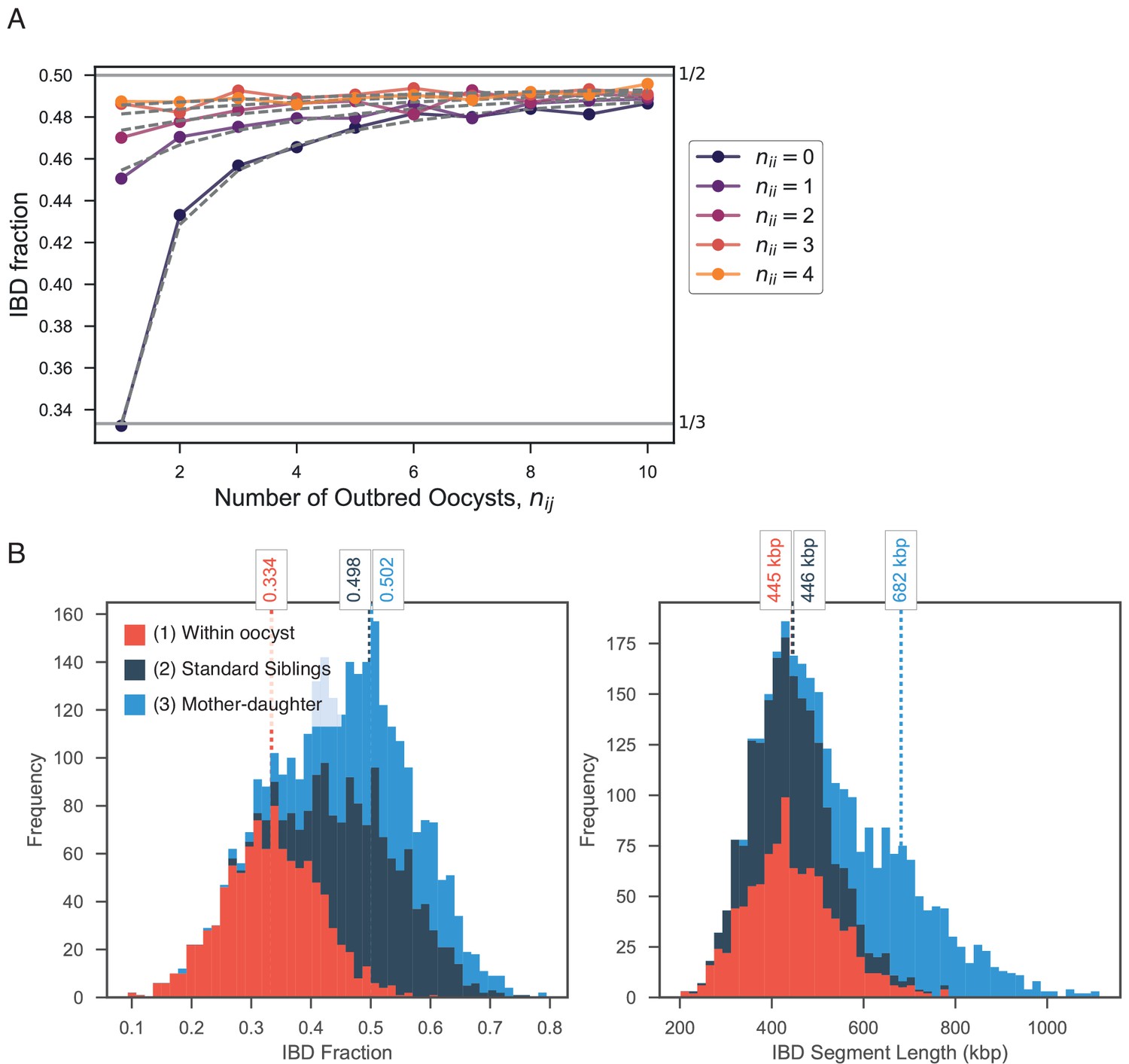
Exploring expected IBD allowing for outbred () and inbred () oocysts.
(A) Validation of expression for expected IBD fraction conditional on outbred and inbred oocysts (S1.9). Line plot compares trend in expected IBD fraction with varying number of outbred (x-axis, ) and inbred (line color, ) oocysts and the analytical expression S1.9 (grey dashed lines). (B) Using pf-meiosis to simulate mixed infections generated from (1) two strains from the same outbred oocyst from (, ’Within oocyst’); (2) two strains different outbred oocysts(, ’Standard Siblings’); (3) one strain from an outbred and one strain from an inbred oocyst (, ’Mother-daughter’).
Tables
Table 1
Summary of Pf3k samples in data release 5.1, where denotes mean read depth and is sample size.
Genotyping, including both indel and SNP variants, was performed using a pipeline based on GATK best practices, see Materials and methods. Data available from ftp://ngs.sanger.ac.uk/production/pf3k/release_5/5.1. is the inferred parasite prevalence rate in a 5 × 5 km resolution grid from the MAP project, centred at the Pf3k sample collection sites; Relatedness and effective number of strains are summary metrics from DEploidIBD output.
| Country | Year | Location | (s.e.) | Reference | ||||
|---|---|---|---|---|---|---|---|---|
| Gambia | 2008 | Brikam | 0.06 | 65 | 129 ( 9.4 ) | 0.5 | 1.3 | (Amambua-Ngwa et al., 2012) |
| Ghana | 2009 | Navrongo | 0.79 | 121 | 86 ( 5.7 ) | 0.21 | 1.6 | (Duffy et al., 2015; Kamau et al., 2015; MalariaGEN Plasmodium falciparum Community Project, 2016) |
| 2010 | Navrongo | 0.79 | 171 | 127 ( 10.3 ) | 0.23 | 1.5 | ||
| 2011 | Navrongo | 0.72 | 97 | 76 ( 5.3 ) | 0.21 | 1.5 | ||
| Kintampo | 0.58 | 6 | 89 ( 13.5 ) | 0.11 | 1.5 | |||
| 2012 | Navrongo | 0.52 | 47 | 111 ( 3.8 ) | 0.29 | 1.6 | ||
| Kintampo | 0.41 | 40 | 157 ( 8.1 ) | 0.22 | 1.6 | |||
| 2013 | Navrongo | 0.31 | 88 | 119 ( 4 ) | 0.26 | 1.6 | ||
| Kintampo | 0.29 | 4 | 172 ( 38.4 ) | 0.44 | 1.1 | |||
| Malawi | 2011 | Chikwawa | 0.19 | 230 | 101 ( 3 ) | 0.26 | 1.7 | (Ocholla et al., 2014) |
| Zomba | 0.34 | 35 | 89 ( 9.1 ) | 0.24 | 1.6 | |||
| Mali | 2007 | Bandiagara | 0.43 | 9 | 95 ( 25.2 ) | 0.39 | 1.8 | (Mobegi et al., 2014; MalariaGEN Plasmodium falciparum Community Project, 2016) |
| Faladje | 0.37 | 36 | 75 ( 10.1 ) | 0.27 | 1.3 | |||
| Kolle | 0.21 | 51 | 82 ( 10.5 ) | 0.3 | 1.6 | |||
| Guinea | 2011 | Nzerekore | 0.49 | 97 | 77 ( 4.6 ) | 0.17 | 1.4 | |
| Congo DR | 2013 | Kinshasa | 0.24 | 113 | 49 ( 3.2 ) | 0.31 | 1.5 | |
| Senegal | 2004 | Thies | 0.09 | 2 | 130 ( 68.2 ) | 0.01 | 1.4 | (Wong et al., 2017) |
| 2009 | Thies | 0.04 | 43 | 175 ( 14.9 ) | 0.43 | 1.1 | ||
| 2010 | Thies | 0.04 | 24 | 159 ( 9.7 ) | 0.3 | 1.3 | ||
| 2011 | Thies | 0.03 | 32 | 97 ( 6 ) | 0.33 | 1.1 | ||
| West | 2009 | Pursat | 0.0071 | 19 | 75 ( 8.8 ) | 0.39 | 1.3 | (Amato et al., 2017; MalariaGEN Plasmodium falciparum Community Project, 2016) |
| Cambodia | 2010 | Pursat | 0.0071 | 105 | 95 ( 6.8 ) | 0.65 | 1.2 | |
| 2011 | Pailin | 0.0025 | 49 | 54 ( 4.1 ) | 0.43 | 1.1 | ||
| Pursat | 0.0096 | 103 | 49 ( 3.1 ) | 0.63 | 1.2 | |||
| 2012 | Pailin | 0.00096 | 31 | 46 ( 5.6 ) | 0.43 | 1.0 | ||
| Pursat | 0.0079 | 7 | 37 ( 19.1 ) | 0.58 | 1.4 | |||
| North | 2010 | Ratanakiri | 0.0039 | 50 | 71 ( 6.1 ) | 0.43 | 1.3 | |
| Cambodia | 2011 | Preah Vihear | 0.02 | 73 | 51 ( 5.3 ) | 0.36 | 1.2 | |
| Ratanakiri | 0.0032 | 81 | 45 ( 4.3 ) | 0.47 | 1.4 | |||
| 2012 | Preah Vihear | 0.0075 | 30 | 43 ( 6.7 ) | 0.37 | 1.0 | ||
| Ratanakiri | 0.0016 | 15 | 44 ( 8.9 ) | 0.3 | 1.3 | |||
| Thailand | 2011 | Mae Sot | 0.00011 | 35 | 66 ( 7.5 ) | 0.35 | 1.2 | (Miotto et al., 2013; MalariaGEN Plasmodium falciparum Community Project, 2016) |
| Sisakhet | 1e-04 | 5 | 112 ( 25.4 ) | 0.17 | 1.3 | |||
| 2012 | Mae Sot | 5.7e-05 | 69 | 83 ( 4.9 ) | 0.58 | 1.3 | ||
| Ranong | 0.00018 | 11 | 82 ( 12.4 ) | 0.38 | 1.2 | |||
| Sisakhet | 0 | 13 | 89 ( 13 ) | 0.37 | 1.1 | |||
| 2013 | Sisakhet | 0 | 3 | 62 ( 8.8 ) | 0.09 | 1.2 | ||
| Bangladesh | 2012 | Ramu | 0.0021 | 50 | 53 ( 4.2 ) | 0.45 | 1.5 | |
| Viet Nam | 2011 | Bu Gia Map | 0.0073 | 43 | 67 ( 5 ) | 0.43 | 1.3 | |
| Phuoc Long | 0.0053 | 27 | 68 ( 7.2 ) | 0.37 | 1.2 | |||
| 2012 | Bu Gia Map | 0.0072 | 19 | 115 ( 8 ) | 0.67 | 1.1 | ||
| Phuoc Long | 0.0048 | 5 | 107 ( 6.3 ) | 0.81 | 1.2 | |||
| Myanmar | 2011 | Bago Division | 0.0076 | 12 | 59 ( 7.1 ) | 0.24 | 1.2 | |
| 2012 | Bago Division | 0.0084 | 47 | 62 ( 5.2 ) | 0.45 | 1.2 | ||
| Laos | 2011 | Attapeu | 0.0094 | 59 | 71 ( 4.2 ) | 0.36 | 1.4 | |
| 2012 | Attapeu | 0.02 | 25 | 77 ( 7.2 ) | 0.68 | 1.3 |
Appendix 1—table 1
Notation used in this article.
https://doi.org/10.7554/eLife.40845.021| Marker index | |
| Sample index | |
| Read count for reference allele | |
| Read count for alternative allele | |
| Population level allele frequency (PLAF) | |
| Number of distinct strains within sample | |
| Number of sites | |
| Proportions of strains | |
| Log titre of strains | |
| Allelic states of parasite strains at site | |
| Allelic state of parasite strain at site | |
| Observed within sample allele frequency (WSAF) | |
| Unadjusted expected WSAF | |
| Adjusted expected WSAF | |
| Probability of read error | |
| IBD configuration at site | |
| Probability of non-IBD in a mixture of two strains |
Appendix 1—table 2
IBD configurations for two, three and four strains, ordered top to bottom by the number of IBD pairs.
The (zero-indexed) notation indicates the type assigned to each haplotype, thus 0–1 indicates non-IBD for two strains, while 0-1-2-2 indicates four strains in which the third and fourth are IBD.
| Index | IBD state | ||
|---|---|---|---|
| K = 2 | K = 3 | K = 4 | |
| 0 | 0–1 | 0-1-2 | 0-1-2-3 |
| 1 | 0–0 | 0-0-1 | 0-0-1-2 |
| 2 | 0-1-0 | 0-1-0-2 | |
| 3 | 0-1-1 | 0-1-2-0 | |
| 4 | 0-0-0 | 0-1-1-2 | |
| 5 | 0-1-2-1 | ||
| 6 | 0-1-2-2 | ||
| 7 | 0-0-1-1 | ||
| 8 | 0-1-0-1 | ||
| 9 | 0-1-1-0 | ||
| 10 | 0-0-0-1 | ||
| 11 | 0-0-1-0 | ||
| 12 | 0-1-0-0 | ||
| 13 | 0-1-1-1 | ||
| 14 | 0-0-0-0 | ||
Appendix 3—table 1
Number of haplotypes discarded and retained for each population in the Pf3k dataset.
https://doi.org/10.7554/eLife.40845.032| Country | Discarded | Retained | Fraction discarded |
|---|---|---|---|
| Bangladesh | 25 | 69 | 0.27 |
| Cambodia | 108 | 697 | 0.13 |
| DR. of Congo | 62 | 155 | 0.29 |
| Ghana | 493 | 609 | 0.45 |
| Guinea | 79 | 88 | 0.47 |
| Laos | 28 | 110 | 0.20 |
| Malawi | 233 | 341 | 0.41 |
| Mali | 37 | 140 | 0.21 |
| Myanmar | 7 | 71 | 0.09 |
| Senegal | 2 | 167 | 0.01 |
| Thailand | 28 | 169 | 0.14 |
| The Gambia | 22 | 73 | 0.23 |
| Vietnam | 23 | 113 | 0.17 |
| Total | 1147 | 2802 | 0.29 |
Appendix 3—table 2
Number of haplotypes retained and discarded stratified by COI level.
https://doi.org/10.7554/eLife.40845.033| COI | Retained | Discarded | Fraction discarded |
|---|---|---|---|
| 1 | 1331 | 34 | 0.02 |
| 2 | 669 | 291 | 0.30 |
| 3 | 583 | 533 | 0.48 |
| 4 | 219 | 289 | 0.57 |
| Total | 2802 | 1147 | |
| Fraction | 0.71 | 0.29 |
Additional files
-
Supplementary file 1
About the Pf3k Project.
- https://doi.org/10.7554/eLife.40845.018
-
Transparent reporting form
- https://doi.org/10.7554/eLife.40845.019
Download links
A two-part list of links to download the article, or parts of the article, in various formats.
Downloads (link to download the article as PDF)
Open citations (links to open the citations from this article in various online reference manager services)
Cite this article (links to download the citations from this article in formats compatible with various reference manager tools)
The origins and relatedness structure of mixed infections vary with local prevalence of P. falciparum malaria
eLife 8:e40845.
https://doi.org/10.7554/eLife.40845


