The genetic architecture of host response reveals the importance of arbuscular mycorrhizae to maize cultivation
- Departamento de Biotecnología y Bioquímica, Centro de Investigación y de Estudios Avanzados del Instituto Politécnico Nacional (CINVESTAV-IPN), Mexico
- Laboratorio Nacional de Genómica para la Biodiversidad/Unidad de Genómica Avanzada, Centro de Investigación y de Estudios Avanzados, Instituto Politécnico Nacional (CINVESTAV-IPN), Mexico
- Department of Plant Science, The Pennsylvania State University, United States
- Crop Science Centre and Department of Plant Sciences, University of Cambridge, United Kingdom
Figures
Figure 1 with 3 supplements
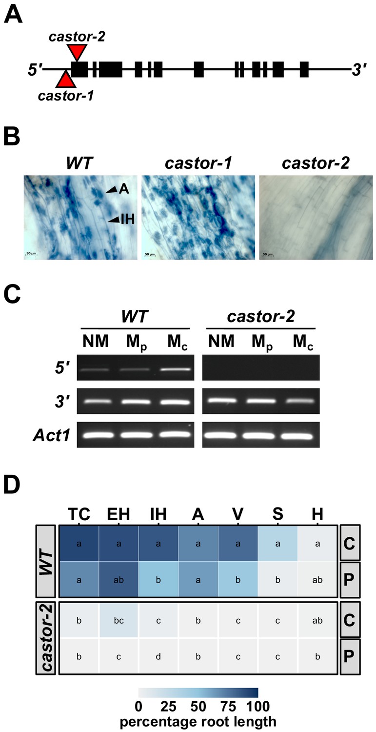
Mutation of maize Castor results in resistance to AMF.
(A) Schematic representation of the maize Castor gene (GRMZM2G099160_T01 gene model). Boxes indicate coding regions. Red triangles indicate the insertion of Mutator transposable elements in the alleles castor-1 and castor-2. (B) Root segments stained with trypan blue 7 weeks after inoculation with Rhizophagus irregularis. Characteristic root-internal hyphal structures, such as intraradical hyphae (IH) and arbuscules (A) , seen in wild-type (WT) and castor-1 plants are absent from the castor-2 mutant. (C) RT-PCR analysis of Castor transcript accumulation in the roots of WT and castor-2 plants that were non-inoculated (NM) or inoculated with plate (Mp. In vitro produced) or crude (Mc. Sand-pot produced) inoculum. Castor cDNA was amplified using a primer set spanning the castor-2 mutator insertion site (5’) and a second set spanning the 3’-most intron (3’). Primers to the maize actin gene Act1 were used as a control. (D) Colonization by AMF (% root length) of the plants analyzed in C. TC, total colonization; EH, external hyphae; IH, internal hyphae; A, arbuscules; V, vesicles; S, spores; H, hyphapodia. C, crude inoculum. P, plate inoculum. Lowercase letters indicate significant differences among genotypes and inoculum, determined by the Kruskal-Wallis test and LSD.
Figure 1—figure supplement 1
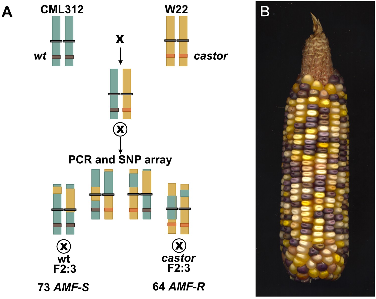
Generation of the F2:3 population.
(A) An F1hybrid was generated from the cross between the CML312 inbred line and a plant homozygous for the castor-2 allele in the W22 background. The F1 was self-pollinated to generate an F2 stock segregating castor-2 along with CML312 and W22 genome content. Homozygous wild-type and mutant individuals were identified by PCR genotyping and self-pollinated to generate F2:3 families. Additional tissue from the F2 parents was used for genotypic analysis on an Illumina 3047 SNP microarray chip as described in the main text. (B) An F2 ear from the cross of the color-converted bz-mum9 Uniform Mu stock carrying castor-2 and the white-kernelled subtropical inbred line CML312.
Figure 1—figure supplement 2
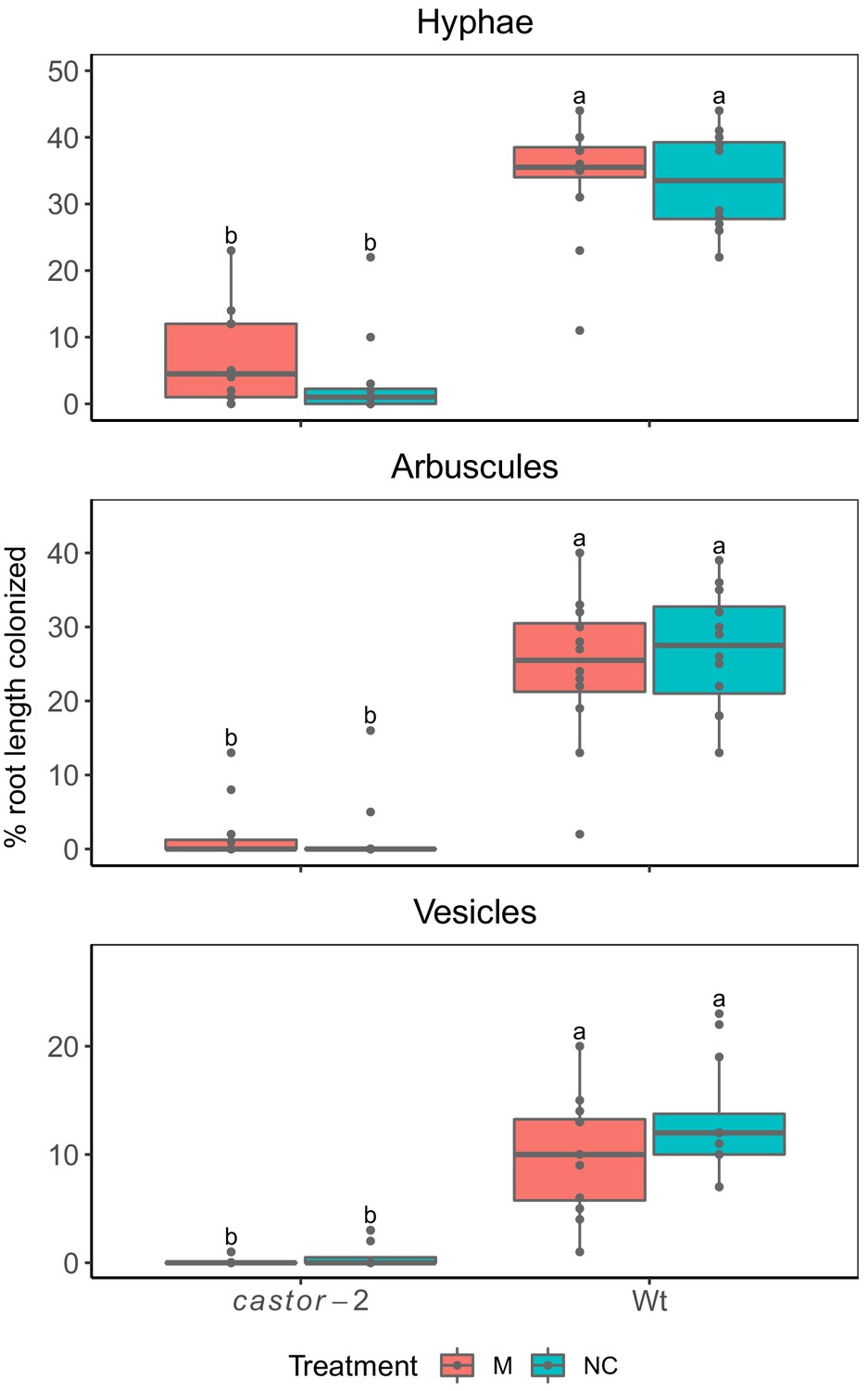
Maize castor-2 mutants are resistant to colonization by AMF.
Field evaluation of castor-2 mutants, Irapuato, Mexico. Two complete blocks with four treatments were used: (1) AMF-S (wt) families without inoculation with exogenous AMF (NC), (2) AMF-R families (castor-2) without inoculation with AMF (NC), (3) AMF-S families (wt) with inoculation with AMF (M), and (4) AMF-R families (castor-2) with inoculation of AMF (M). The inoculum used was the commercial consortium BioMic which includes: Glomus constrictum, Glomus geosporum, Glomus tortuosum, Acaulospora scrobiculata, Gigaspora margarita, and Glomus sp. Field colonization of wt families without application of exogenous inoculum indicates the action of the native community of AMF.
Figure 1—figure supplement 3
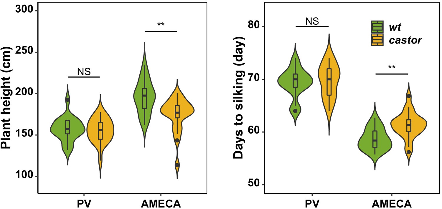
Evaluation of AMF-S (wt) and AMF-R (castor) families in heavily managed (PV) and a rain-fed, medium input (Ameca) fields.
A subset of 20 AMF-S and 20 AMF-R families was evaluated in a winter season in a managed (fertigation, herbicide, pesticide; sandy soil allowing free availability of nutrients to plants) field site near Puerto Vallarta on the Mexican Pacific Coast. No difference was seen between AMF-S and AMF-R families in plant height or days-to-silking (female flowering). By contrast, in the medium-input Ameca site used for the full evaluation, AMF-S and AMF-R families were distinct. The box in violin plots represents the interquartile range with the horizontal line representing the median and whiskers extend 1.5 times the interquartile ranges. The shape of the violin plot represents the probability density of data at different values along the y-axis. Results were based on two-group Wilcoxon tests with Bonferonni adjusted p-values. Note: *: p<0.05; **: p<0.01; ***: p<0.001; NS: not significant.
Figure 2 with 6 supplements
Mycorrhizal symbiosis promotes maize growth under cultivation.
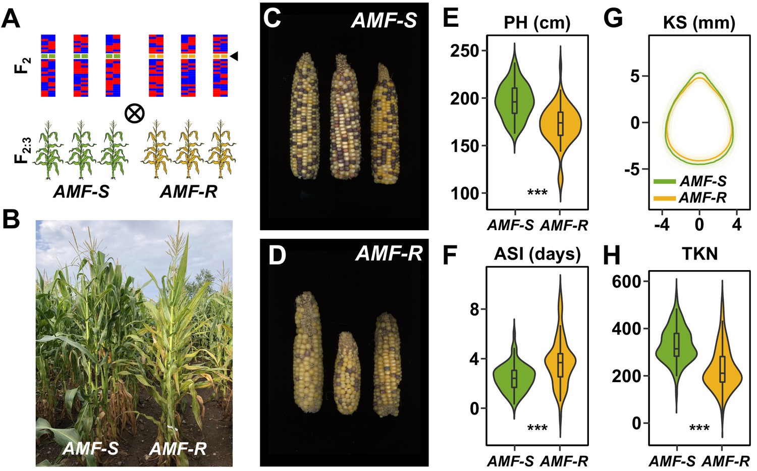
(A) Susceptible (AMF-S) and resistant (AMF-R) families segregate genomic content from two founder parents, shown as red and blue bars, but are homozygous for the wild-type (green) or mutant (yellow) allele at Castor (black arrow), respectively, blocking AM symbiosis in AMF-R. (B), Border between representative AMF-S and AMF-R plots, Ameca, Mexico, 2019. (C), Representative AMF-S ears. (D), Representative AMF-R ears. (E), Plant height (PH) of 73 AMF-S (green) and 64 AMF-R (yellow) families. (F), Anthesis-silking interval (ASI). (G), Kernel shape (KS) based on the analysis of scanned kernel images . (H), Total kernel number (TKN). The violin plots in (E, F and H) are a hybrid of boxplot and density plot. The box represents the interquartile range with the horizontal line representing the median and whiskers extending 1.5 times the interquartile range. The shape of the violin plot represents the probability density at different values along the y-axis. ***, difference between AMF-S and AMF-R significant at p<0.001 (Wilcoxon test; Bonferonni adjustment based on the total trait number).
Figure 2—figure supplement 1
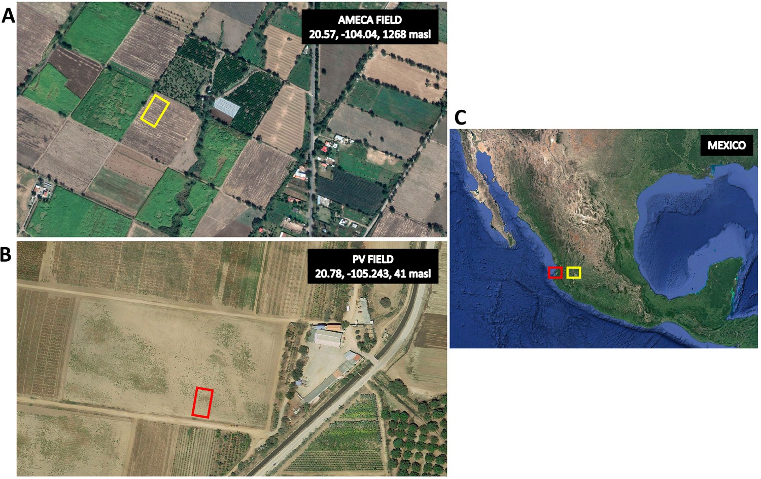
Location of experimental fields.
(A) Satellite view of the Ameca site used for the principal field evaluation (20.57 lat, −104.04 lon, 1268 masl). Yellow rectangle shows the field area. (B) Satellite view of the Puerto Vallarta (PV) site used for population generation and preliminary high-input evaluation (20.78 lat, −105.243 lon, 41 masl). Red rectangle shows the field area. (C) Mexico showing the two sites.
Figure 2—figure supplement 2
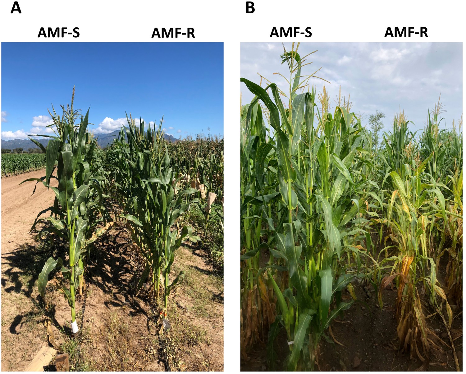
Representative AMF-S and AMF-R families in high- and medium- input sites.
(A) Winter PV field in 2020, located in Nayarit, Mexico. (B) Summer Ameca field in 2019, located in Jalisco, Mexico.
Figure 2—figure supplement 3
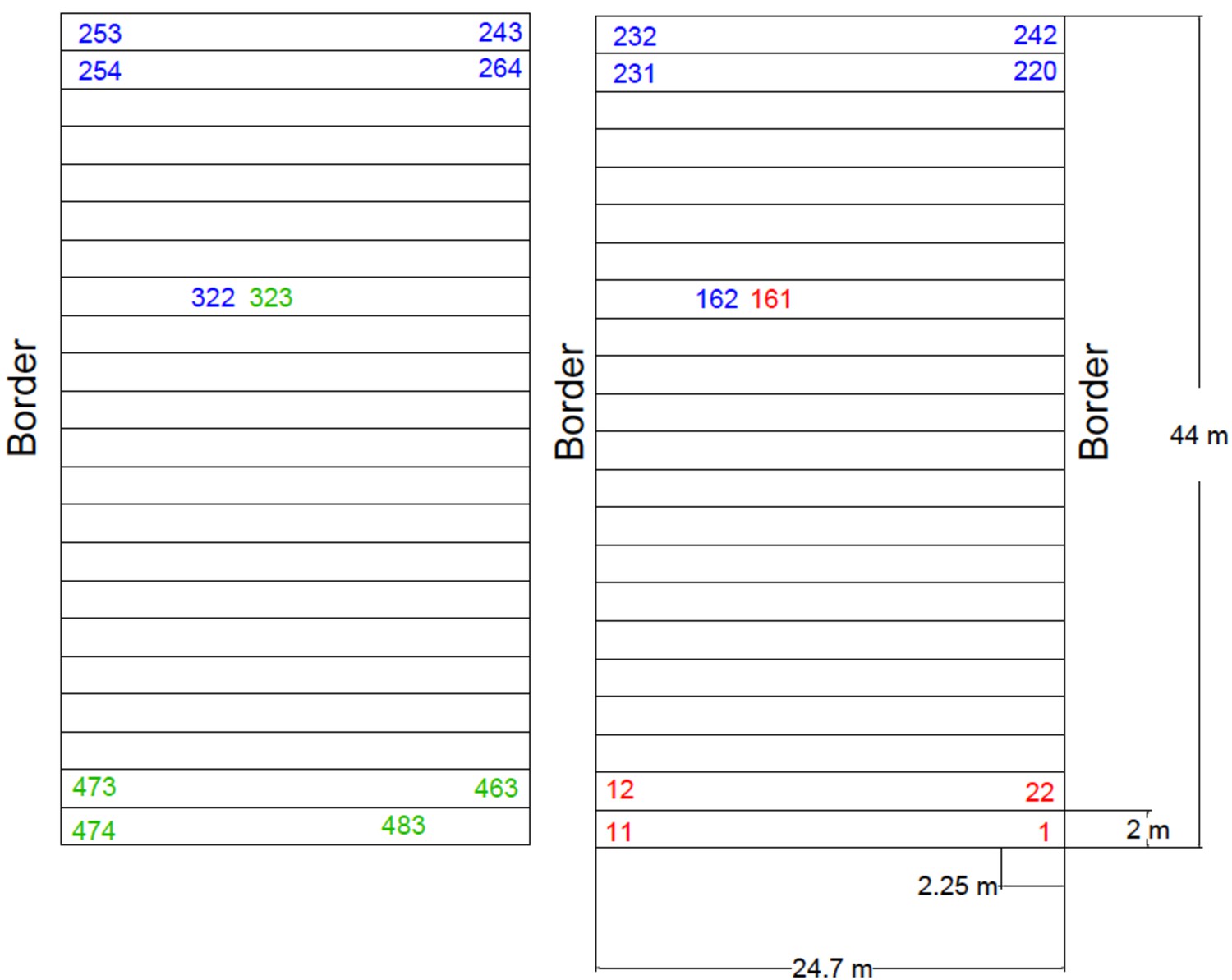
Plan of the Ameca field design.
Summer experimental field 2019, located in Ameca, Jalisco. Three complete blocks were evaluated. Forty-five seeds were sown per three-row plot (15 seed per row). AMF-S and AMF-R families were alternated with the order of the families within each subpopulation randomized within each block. The rows marked with red, blue, and green correspond to blocks 1, 2, and 3, respectively. A commercial UNISEM hybrid was planted on the border of the experiment and used as a check throughout the field. The field was fertilized at planting with 250 kg / Ha of diammonium phosphate (DAP) as a source of nitrogen and phosphorus (18-46-00, NPK). A further application of 250 kg / Ha of urea was given (46-00-00, NPK) at 40 days after planting.
Figure 2—figure supplement 4
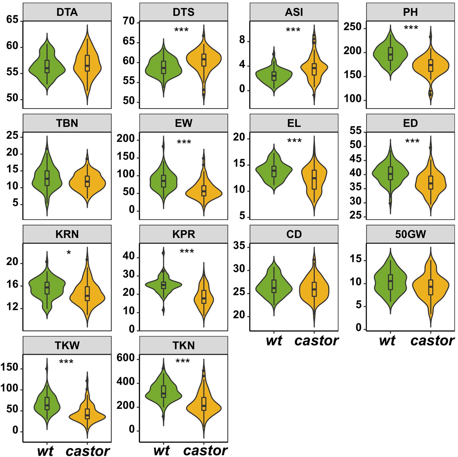
Comparison of plant phenotypic traits between AMF-S (wt) and AMF-R (castor) families.
The box in violin plots represents the interquartile range with the horizontal line representing the median and whiskers representing 1.5 times the interquartile ranges. The shape of the violin plot represents the probability density of data at different values along the y-axis. Results were based on two-group Wilcoxon tests with Bonferonni adjusted p-values. Note: *: p<0.05; **: p<0.01; ***: p<0.001; NS: not significant. Trait codes as in Table 1.
Figure 2—figure supplement 5

Ear and kernel image analysis.
The shape of maize ear (A), cob (B), and kernel (C) of AMF-S (wt) and AMF-R (castor) families. Median shapes of ear, cob, and kernel from two families were shown in thick green and yellow lines, whereas individual genotypes of two groups were shown in thin, semi-transparent green, and yellow lines. Shapes were extracted from scanned images from 3 ears per plot, 50 kernels per ear.
Figure 2—figure supplement 6
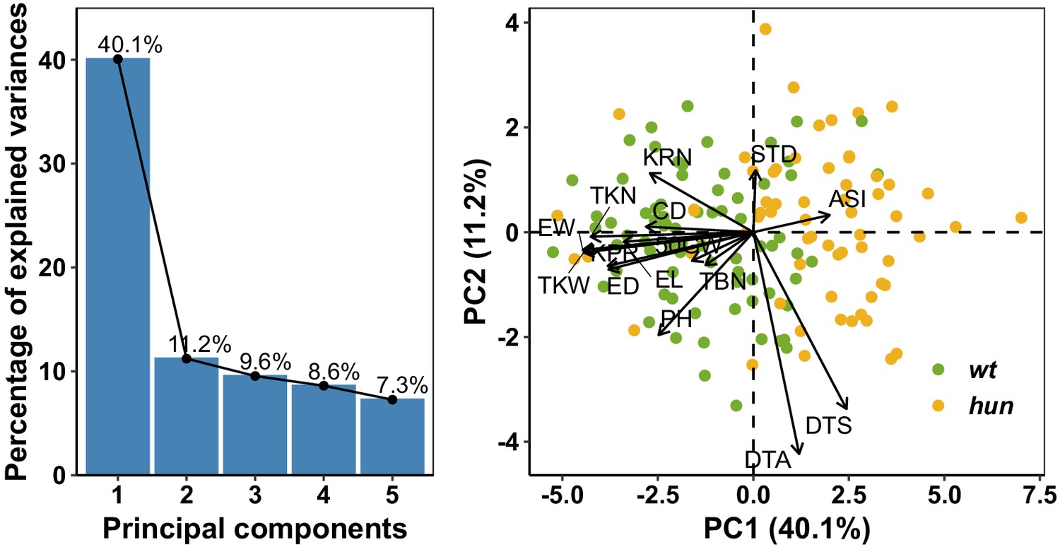
Principal component analysis.
A, Phenotypic variation captured by the first five principal components (PCs). The first two principal components (PCs) explained more than 50% of the phenotypic variance. PC1 (40.1%) was primarily associated with ASI and maize yield-related traits, such as ear weight (EW), total kernel number (TKN), and total kernel weight (TKW). B, Loading of AMF-S and AMF-R families on PC1 and PC2. The position of trait names (as Table 1) with respect to the origin indicates contribution to each PC.
Figure 3 with 2 supplements
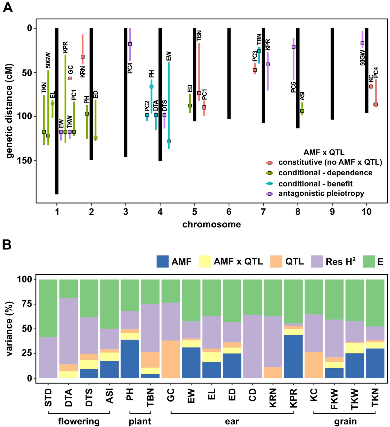
QTL x AMF effects contribute significantly to variation in host response.
(A) Genomic position of QTL identified in this study. Boxes indicate the position of the peak marker. Bars represent the drop-1 LOD interval. Colors denote patterns of AMF × QTL interaction as described in the text. (B) The contribution of different components to phenotypic variance in different plant traits among AMF-S and AMF-R families. Total genetic variance was estimated based on differences between experimental blocks and partitioned into variation explained by the additive effect of AMF, the additional variation explained by interactive QTL and QTL × AMF interaction (QTL × AMF), the additional variation explained by additive QTL (QTL) and residual genetic variation (Res H2). The balance of the phenotypic variance was assigned to the environment (E). Traits codes as in Table 1.
-
Figure 3—source data 1
QTL analysis.
LOD plots of the single-scan QTL performed on the 17 traits studied (see Supplementary file 1 Table S2 for trait codes). The color of the line represents the different models considered: AMF-S families only (H0wt, blue line), AMF-R only (H0hun, red line), AMF as an additive covariate (Ha, yellow line), AMF as an interactive covariate (Hf, purple line), and the evidence of interaction (Hi, green line). The solid line represents the QTL and drop 1-LOD confidence interval. The horizontal dotted line represents the LOD threshold obtained with a 1000 permutations(α = 0.05) for H0wt, H0hun, Ha, and Hf and calculated as LOD_thri = LOD_thrf - LOD_thra for Hi.
- https://cdn.elifesciences.org/articles/61701/elife-61701-fig3-data1-v1.pdf
Figure 3—figure supplement 1
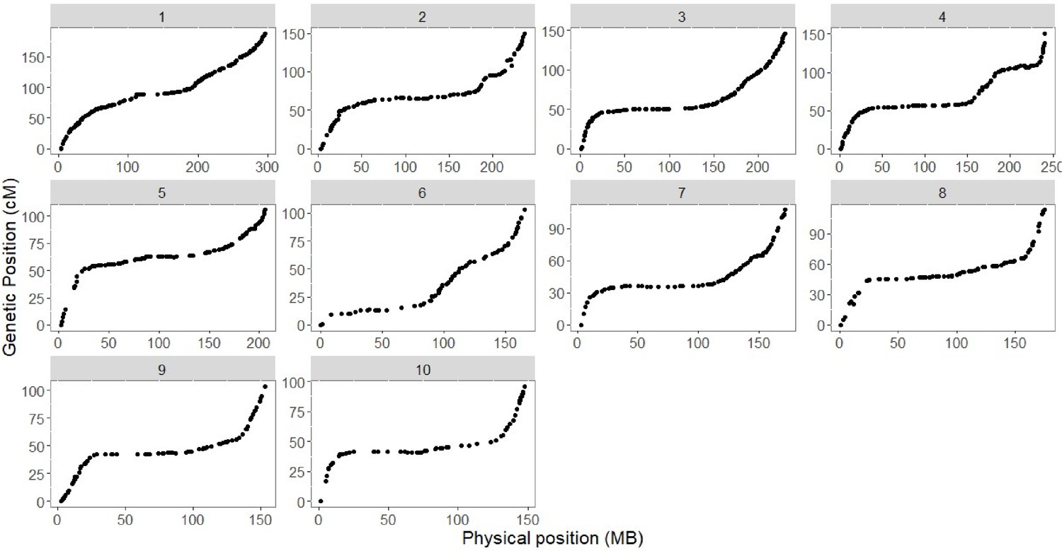
Genotypic analysis.
Plot of genetic (y axis) and physical (x axis) position for 1050 genetic markers that compose the genetic map of the CML312 x W22 castor-2 F2 population.
Figure 3—figure supplement 2
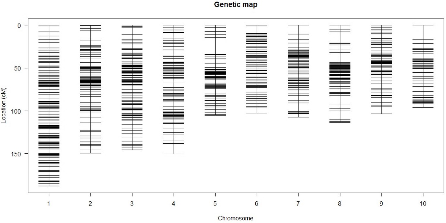
Genetic map.
Plot representing the estimated genetic map and the marker distribution across the ten chromosomes of maize for the CML312 × W22 castor-2 F2 population.
Figure 4 with 1 supplement

Mycorrhiza response confounds benefit and dependence.
(A) Host response (R) is the difference in trait value between mycorrhizal (M; green) and non-mycorrhizal (NM, yellow) plants. Increased response can result from either greater dependence (D; poorer performance of NM plants) or greater benefit (B; greater performance of M plants). (B), QTL × AMF effects underlying variation in response reveal the balance of benefit and dependence. In this theoretical example, the effect is conditional on mycorrhizal colonization, reflecting a difference in benefit more than dependence. (C, D) Effect plots for major QTL associated with PC1 and PC2, respectively. Effect of the homozygous CML312 (red), homozygous W22 (blue), or heterozygous (brown) genotypes in AMF-S and AMF-R families. The PC1 QTL is conditional on AMF-R, indicating a difference in dependence. The PC2 QTL is conditional on AMF-S, indicating a difference in benefit.
-
Figure 4—source data 1
QTL analysis.
Effect plots for major QTL detected in the analysis across susceptible (AMF-S) and resistant (AMF-R) families. The title of the plot gives the marker nearest to the LOD peak, and the color of the line represents the genotype at the QTL.
- https://cdn.elifesciences.org/articles/61701/elife-61701-fig4-data1-v1.pdf
Figure 4—figure supplement 1
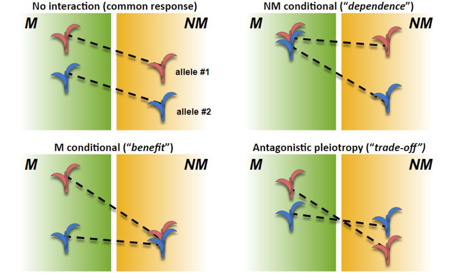
Scenarios in AMF x genotype interaction.
Theoretical performance (arbitrary units; y axis) of mycorrhizal (M) and non-mycorrhizal (NM) plants of two genotypes (red and blue). The difference between M and NM defines response for a given genotype. (Top left) No AMF × genotype interaction. Both genotypes respond equally to AMF; the difference between varieties is constant between M and NM. (Top right) NM conditional. Response is higher in the blue genotype; difference between genotypes is conditional on NM treatment; response variation is driven by greater dependence of the blue genotype. (Bottom left) M conditional. Response is higher in the red genotype; difference between genotypes is conditional on M treatment; response variation is driven by greater benefit of the blue genotype. (Bottom right) Antagonistic pleiotropy. Response is higher in the red genotype; difference between the genotypes is expressed in both M and NM, but the sign of the effect changes; the red genotype is superior in M growth but inferior in NM growth.
Figure 5

The genetic architecture of mycorrhiza response implies a trade-off between dependence and benefit.
(A) Extreme QTL × AMF effects result in antagonistic pleiotropy. In this theoretical example, the blue allele is superior in mycorrhizal (M) plants, while the red allele is superior in non-mycorrhizal (NM) plants. Such a QTL is linked to differences in both dependence and benefit. (B) Effect plot for a total kernel weight (TKW) QTL located on Chromosome 1. TKW of families homozygous for the CML312 allele at this locus (red) is stable across susceptible (AMF-S) and resistant (AMF-R) families. In contrast, families homozygous for the W22 allele (blue) or heterozygous at this locus (brown), show superior TKW if AMF-S but lower TKW if AMF-R. (C) Theoretical trade-off between the performance of non-mycorrhizal (NM) and mycorrhizal (M) plants. For any position on this plot, the vertical distance above the diagonal indicates the magnitude of host response. Trade-off prevents occupancy of the upper-right of the plot, defining a so-called ‘Pareto front’ (solid arc). Here an increase in the NM performance of variety X is necessarily accompanied by a reduction in M performance, as described by movement along the arc to condition Y. Biological constraint prevents the path towards condition Z. (D) Fitted ear weight values for all genotypes from a multiple QTL model under both levels of AMF (AMF-S and AMF-R). Line segments connect the same plant genotype under the two AMF levels. (E) Observed ear weight against whole-genome prediction for 73 susceptible (AMF-S) and 64 resistant (AMF-R) families. Best fit regression line in dashed blue. (F) Predicted ear weights for all 137 genotypes based on AMF-S (M) and AMF-R (NM) whole-genome models. Dashed red line shows AMF-S = AMF R, that is, no host response.
Tables
Table 1
Summary of the host response and QTLs.
| Trait | Mean AMF-S | Mean AMF-R | Adj. P-value1 | HR2 | HR (%)3 | QTLs4 | AMFxQTL5 | Chr6 | Type7 |
|---|---|---|---|---|---|---|---|---|---|
| STD | 11 | 10 | NS | 1 | 10 | 0 | 0 | ||
| DTA | 56 | 57 | NS | -1 | -1 | 1 | 1 | 4 | B |
| DTS | 59 | 60 | *** | -1 | -3 | 1 | 1 | 4 | AP |
| ASI | 2 | 4 | *** | -2 | −34 | 1 | 1 | 8 | D |
| PH | 196.8 | 171.8 | *** | 25 | 15 | 2 | 2 | 2, 4 | D, B |
| TBN | 13 | 12 | NS | 1 | 10 | 2 | 1 | 5, 7, | B |
| GC | 0. 56 | 0. 4 | NS | 0.15 | 38 | 1 | 0 | 1 | |
| EW | 86.6 | 60.6 | *** | 26 | 43 | 2 | 2 | 1, 4 | AP, B |
| EL | 13.9 | 12.4 | *** | 1.5 | 13 | 1 | 1 | 1 | D |
| ED | 40.3 | 37.2 | *** | 3.1 | 8 | 2 | 2 | 2, 5 | D, D |
| KRN | 16 | 15 | * | 1 | 6 | 1 | 0 | 2 | |
| KPR | 25 | 18 | *** | 7 | 37 | 2 | 2 | 1, 7 | D, AP |
| KC | 0. 3 | 0.23 | NS | −0.06 | 21 | 1 | 0 | 10 | |
| CD | 26.6 | 26.1 | NS | 0.5 | 2 | 0 | 0 | ||
| FKW | 10.4 | 9.4 | NS | 1 | 10 | 2 | 2 | 1, 10 | D, AP |
| TKW | 67.7 | 44.8 | *** | 22.9 | 51 | 1 | 1 | 1 | AP |
| TKN | 330 | 230 | *** | 100 | 44 | 1 | 1 | 1 | D |
| PC1 | −1.23 | 1.7 | *** | 2 | 1 | 1, 5 | D | ||
| PC2 | 0.126 | −0.182 | NS | 1 | 1 | 4 | B | ||
| PC3 | 0.251 | −0.288 | * | 1 | 0 | 7 | |||
| PC4 | −0.033 | 0.037 | NS | 2 | 1 | 3, 10 | AP | ||
| PC5 | −0.245 | 0.282 | *** | 1 | 1 | 8 | AP |
-
1Wilcoxon tests with Bonferonni adjusted p-values. Note: *: p<0.05; **: p<0.01; ***: p<0.001; NS: not significant. 2Host response calculated as mean AMF-S - AMF-R. 3Host response expressed as a percentage of AMF-R mean. 4Number of QTL associated with a given trait. 5Number of QTL showing significant QTL x AMF effect. 6Chromosomes where the QTLs are located. 7Pattern of QTL x AMF effect: D: dependence QTL expressed primarily in AMF-R families; B, benefit QTL expressed primarily in AMF-S families; AP, antagonistic pleiotropy. Trait codes: STD, stand count; DTA, days to anthesis; DTS, days to silking; ASI, anthesis-silking interval; PH, plant height; TBN, tassel branch number; EW, ear weight; EL, ear length; ED, ear diameter; KRN, kernel row number; KPR, kernels per row; CD, cob diameter; FKW, fifty kernel weight; TKW, total kernel weight; TKN, total kernel number. PC, principal components from an analysis of all traits, numbered in descending order of variance explained.
Additional files
-
Supplementary file 1
Table S1: Traits measured in this study; Table S2: Trait broad-sense heritability and variance explained by terms in QTL models.
- https://cdn.elifesciences.org/articles/61701/elife-61701-supp1-v1.docx
-
Transparent reporting form
- https://cdn.elifesciences.org/articles/61701/elife-61701-transrepform-v1.docx
Download links
A two-part list of links to download the article, or parts of the article, in various formats.
Downloads (link to download the article as PDF)
Open citations (links to open the citations from this article in various online reference manager services)
Cite this article (links to download the citations from this article in formats compatible with various reference manager tools)
The genetic architecture of host response reveals the importance of arbuscular mycorrhizae to maize cultivation
eLife 9:e61701.
https://doi.org/10.7554/eLife.61701


