Time encoding migrates from prefrontal cortex to dorsal striatum during learning of a self-timed response duration task
Figures
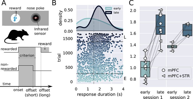
Description of the task and behavioral results.
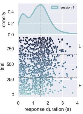
(A) Experimental design used in the experiment. The trial starts when the rat inserts its snout in the nose poke installed next to the reward port. The step lines represent the nose poke onset and offset. Depending on how long the rat stays in the nose poke—the response duration—it may receive access to a sucrose solution. Responses lasting more than 1.5 s grant access to three licks of sucrose solution, while shorter responses produce no consequences. (B) Responses from a single rat in the first session of training in the task. (Lower graph) Each dot represents a response duration (x-axis) in a specific trial (y-axis). The vertical dashed line represents the criterion (1.5 s) for receiving the reward. The two horizontal dash-dotted lines show the trials that were used in the electrophysiology experiments for early ‘E’ and late ‘L.’ (Upper graph) Probability density of responses as a function of the duration for the early and late trials, showing that the distribution shifted to the right. (C) Mean response duration for individual rats early and late in sessions 1 and 2. All animals significantly increased their responses in the very first session of training. For one group of animals (group medial prefrontal cortex [mPFC] + striatum [STR]), we recorded a second day of training. At the beginning of this second session (early trials), animals’ response durations were shorter than the late trials of session 1, but much longer than the early trials, showing that the training from session 1 improved the behavior early in session 2. Throughout the second session, rats achieved the same performance as the late trials of session 1, suggesting that the training in the first session took the rats close to the optimal performance.
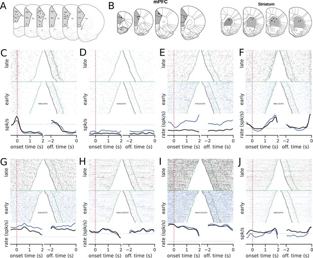
Recording sites and examples of neural activity during trials.
(A) Recording sites in the medial prefrontal cortex (group mPFC). (B) Recording sites for group mPFC + striatum (STR). (C–J) The upper graphs show the raster plots from early (blue) and late (black) trials for mPFC (C–F) and STR (G–J). The bottom graphs show the corresponding firing rates, color-coded. The time scale for raster plots and firing rates consists of recordings starting 500 ms before the rat enters the nose poke and ending when the animal leaves the nose poke. Trials were either aligned to the nose poke entering (onset time, left) or to the instant the rat left the nose poke (offset time, right). In onset time, the zero represents the instant the rat entered and the green points show when the animal left the nose poke. In offset time, the zero represents the instant the rat left the nose poke and, consequently, all times are negative. The green point shows when the animal entered the nose poke and the black markers at the beginning of each trial represent the 500 ms before entering the nose poke. (C) A neuron whose activity is tuned to the trial onset. (D–F) Examples of neurons whose activity within the trial became less sensitive (flatter) in later trials compared with earlier trials in the session.
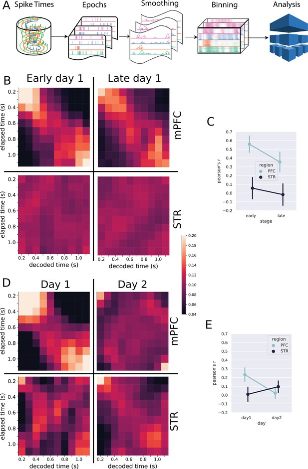
Classification analysis.
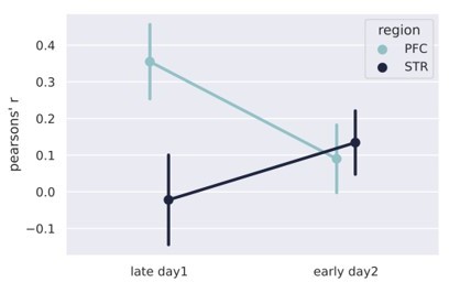
(A) Pipeline of the analysis at the population level. Spike trains are epoched according to the trials, from 0.5 s before nose poke onset through the offset. The epoched trials are shown in Figure 2C–J. The trials are smoothed with a Gaussian kernel (σ = 100 ms) and then binned every 100 ms. The resulting spike rates were analyzed with the linear discriminant analysis. (B, D) Results of the classification decoder analysis within session 1 (B) and between sessions 1 and 2 (D). The confusion matrix (in the form of a heatmap) shows the probability of decoding a particular actual time bin (x-axis) as one of the possible decoding bins (y-axis). A diagonal pattern of bright pixels indicates a better performance of the classifier. (B) Results of the classifier in the medial prefrontal cortex (mPFC) (top row) and striatum (STR) (bottom row), early and late in training showing that the performance decreased with learning. (C) Overall classifier performance for mPFC (blue line) and STR data (black line), measured as a correlation coefficient (Pearson’s R) between the actual and the predicted bin. The results show that the performance decreases in the mPFC while there is no evidence of changes in the STR. Error bars represent the standard deviation of the distributions obtained with a bootstrap procedure (1000 folds). (D, E) Same analysis as in (B, C) but comparing data from sessions 1 and 2, for animals with electrodes implanted in both regions (group mPFC + STR). (E) Decoding performance from mPFC (top row) and STR (bottom row) during day 1 (left column) and day 2 (right column). During day 1, mPFC outperformed the STR in decoding time information. On day 2, the opposite pattern emerged. (E) Pearson’s R score of the decoder performance summarizing results shown in (E).
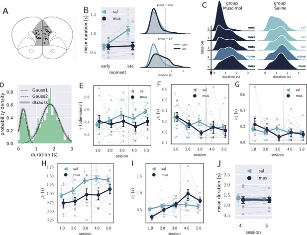
Results from the pharmacological inactivation of the medial prefrontal cortex (mPFC).
(A) Histology showing the microinjection sites in the mPFC. (B) Left: average response duration early and late in the first session for saline (sal, N=8) and muscimol (mus, N=11) groups. Error bars represent the SEM. Right: same data as in left, but combining the responses from all rats for each group. The saline (sal) group increased the response duration during the first session (day 1), while the muscimol (mus) group produced no detectable change in behavior. (C) Probability density of late responses combined from all rats for the five consecutive sessions. The drug injected in each session is at the right of each graph and color-coded. The saline group evolves as expected, producing longer responses from the first session, producing bimodal distribution, whose second peak increases with respect to the first, remaining stable in sessions 3 and 4. The muscimol group has no sign of learning in the first session but progressed after the second session at a slower rate compared to saline group. By session 3, the peak of premature responses is still more prominent than the long (> 1 s) responses. (D) Histogram of response durations from one rat showing the bimodal distribution and the separate fitted distributions representing the premature responses (Gauss1), the temporally controlled responses (Gauss2), and the double Gaussian fit (dGauss). (E–I) Evolution of each double Gaussian parameter as a function of the sessions, γ (E), (F), (G), (H), and (I). The vertical dashed line divides the experiment into two phases: the first (sessions 1–3), when groups received different treatments, and second (sessions 4 and 5) when both groups received the same treatment. (J) Comparison between sessions 4 (no drug) and 5 (muscimol) for the saline (sal) and muscimol (mus) groups, suggesting that the muscimol injection produced no effect on trained animals.
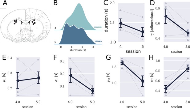
Inactivation of the striatum (STR) in trained animals.
(A) Histological sites for the pharmacological experiments in the STR. (B) Comparison between the combined distribution of responses for trained rats (N=4) in session 4 (no drug) and session 5 (muscimol), showing that the temporally controlled responses were more variable when the STR was inactivated. (C) Mean response duration for sessions 4 (no drug) and 5 (muscimol). (D–H) Parameters obtained with the double Gaussian fit for sessions 4 and 5. The variables and differed in these sessions, showing that the temporally controlled responses spread more with the inactivation of the STR. Errorbars represent the SEM.

Figure with spikes from a neuron that remained stable throughout the session and met the criterion (left) and one that did not (right).
In both figures, the average spike waveform from the beginning of the session is shown in blue and from the end in green. The corresponding shaded areas show the standard deviation of the waveforms.
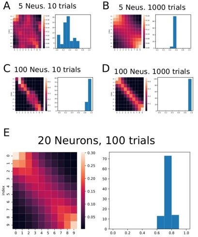
Figure showing the classifier applied to simulated data consisting of several ramping neurons and several trials.
Each graph from A through E shows a result from a different number ofneurons (Neus.) and the number of trials in the simulated data. Generally speaking, the effect of higher decoding probability at the beginning and at the end of the trials persists. On the right of each heat map there is a histogram showing the correlation coefficient obtained in each fold of the data.
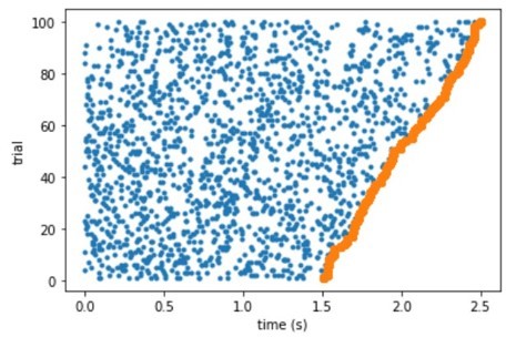
Raster plot of a simulated neuron with uniform response probability density.
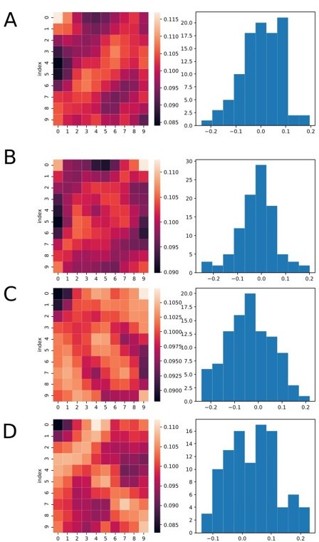
Heatmaps and histograms showing four different runs of the analysis, each for a different set of simulated data.
Neurons were simulated as random spikes uniformly distributed over the entire trial duration. We still can see that many bins at the border (top or down) are brighter. However, the overall mean value of the r coefficient remains zero on average for all cases.
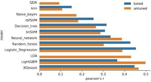
Figure comparing different algorithms decoding the time intervals, as the final pearson’s R coefficient.
Methods used, from top to bottom: QDA: Quadratic Discriminant Analysis,Naive_bayes, rbfSVM:Radial Basis Function kernel SVM, Decision Tree, linSVM: linear SVM, Neural network, Random Forest, Logistic Regression, LDA: linear discriminant analysis, LightGBM: Light Gradient Boosting Machine, and XGboost.
Tables
Number of units selected for analysis per rat, brain region, and day of training.
Rats 7–10 received only one session of training, with recordings in medial prefrontal cortex (PFC). Rats 3–6 trained for two days, with recordings in PFC and striatum (STR). The symbol ‘-’ denotes that no neurons in that specific condition were recorded.
| Day | Rat | 3 | 4 | 5 | 6 | 7 | 8 | 9 | 10 |
|---|---|---|---|---|---|---|---|---|---|
| Region | |||||||||
| 1 | PFC | 4 | 22 | 5 | 4 | 11 | 35 | 10 | 9 |
| STR | 12 | 15 | 16 | 1 | - | - | - | - | |
| 2 | PFC | 14 | 28 | 5 | 3 | - | - | - | - |
| STR | 16 | 16 | 23 | 5 | - | - | - | - | |
| Total | 46 | 81 | 49 | 13 | 11 | 35 | 10 | 9 |
Table with the number of trials for each rat implanted in the STR.
| Dayrat | 1 | 2 |
|---|---|---|
| 3 | 543 | 625 |
| 4 | 341 | 381 |
| 5 | 509 | 437 |
| 6 | 936 | 699 |
Additional files
-
Transparent reporting form
- https://cdn.elifesciences.org/articles/65495/elife-65495-transrepform1-v1.pdf
-
Supplementary file 1
Classification analysis on incorrect trials. The analysis shown here was identical to that in Figure 3 of the main manuscript, except that we only used trials that were shorter than 1.5 s (non-reinforced) and longer than 1s.
- https://cdn.elifesciences.org/articles/65495/elife-65495-supp1-v1.zip


