Research Article

Neuroscience

Mapping brain-behavior space relationships along the psychosis spectrum

Department of Psychiatry, Yale University School of Medicine, United States
Interdepartmental Neuroscience Program, Yale University School of Medicine, United States
RBNC Therapeutics, United States
Department of Psychology, University of Ljubljana, Slovenia
Faculty of Computer and Information Science, University of Ljubljana, Slovenia
Department of Psychiatry, University of Zagreb, Croatia
Department of Psychiatry, Psychotherapy and Psychosomatics, University Hospital for Psychiatry Zurich, Switzerland
The Janssen Pharmaceutical Companies of Johnson and Johnson, United States
Department of Physics, Yale University, United States
Department of Psychology, Yale University School of Medicine, United States

Jul 20, 2021

https://doi.org/10.7554/eLife.66968

Open access
Copyright information

Figures
Tables
Additional files

38 figures, 5 tables and 1 additional file

Figures

Figure 1

Download asset Open asset

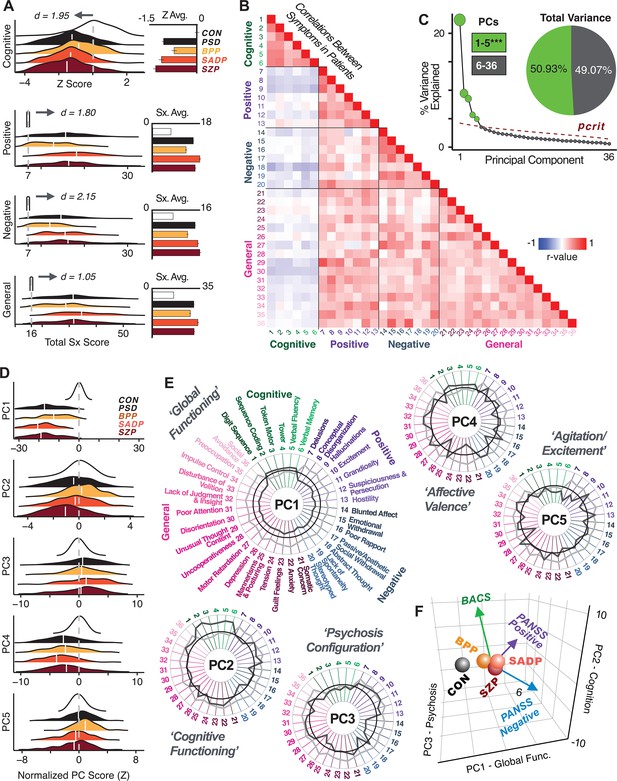
Quantifying data-driven low-dimensional variation of cross-diagnostic psychosis spectrum disorder (PSD) symptoms and cognitive deficits.

(A) Distributions of symptom scores for each of the DSM diagnostic groups across core psychosis symptom measures (PANSS positive, negative, and general symptoms tracking illness severity) and cognitive deficits (BACS composite cognitive performance). BPP: bipolar disorder with psychosis (yellow, N = 150); SADP: schizo-affective disorder (orange, N = 119); SZP: schizophrenia (red, N = 167); All PSD patients (black, N = 436); Controls (white, N = 202). Bar plots show group means; error bars show standard deviations. (B) Correlations between 36 symptom measures across all PSD patients (N = 436). (C) Screeplot shows the % variance explained by each of the principal components (PCs) from a PCA performed using all 36 symptom measures across 436 PSD patients. The size of each point is proportional to the variance explained. The first five PCs (green) survived permutation testing (p<0.05, 5000 permutations). Together they capture 50.93% of all symptom variance (inset). (D) Distribution plots showing subject scores for the five significant PCs for each of the clinical groups, normalized relative to the control group. Note that control subjects (CON) were not used to derive the PCA solution; however, all subjects, including CON, can be projected into the data-reduced symptom geometry. (E) Loading profiles shown in dark gray for the 36 PANSS/BACS symptom measures on the five significant PCs. Each PC (‘Global Functioning’, ‘Cognitive Functioning’, ‘Psychosis Configuration’, ‘Affective Valence’, ‘Agitation/Excitement’) was named based on the pattern of loadings on symptom measures. See Appendix 1—figure 2G for numerical loading values. The PSD group mean score on each symptom measure is also shown, in light gray (scaled to fit on the same radarplots). Note that the group mean configuration resembles the *PC1* loading profile most closely (as *PC1* explains the most variance in the symptom measures). (F) PCA solution shown in the coordinate space defined by the first three PCs. Colored arrows show a priori composite PANSS/BACS vectors projected into the *PC1-3* coordinate space. The a priori composite symptom vectors do not directly align with data-driven PC axes, highlighting that PSD symptom variation is not captured fully by any one aggregate a priori symptom score. Spheres denote centroids (i.e. center of mass) for each of the patient diagnostic groups and control subjects. Alternative views showing individual patients and controls projected into the PCA solution are shown in Appendix 1—figure 2A-F.

Figure 2

Download asset Open asset

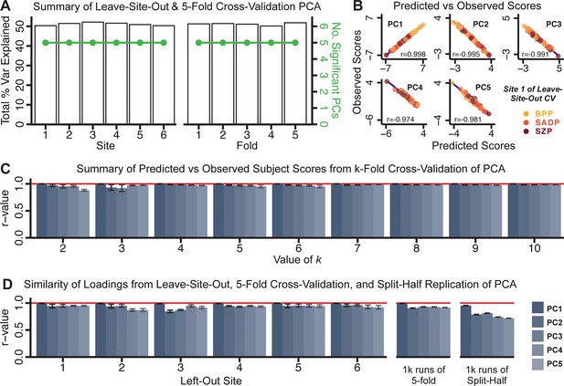
Dimensionality reduction of PSD symptom measures is highly stable and reproducible.

(A) PCA solutions for leave-one-site out cross-validation (left) and 5-fold bootstrapping (right) explain a consistent total proportion of variance with a consistent number of significant PCs after permutation testing. Full results available in Appendix 1—figure 4 and Appendix 1—figure 5. (B) Predicted versus observed single subject PC scores for all five PCs are shown for an example site (shown here for Site 1). (C) Mean correlations between predicted and observed PC scores across all patients calculated via k-fold bootstrapping for k = 2–10. For each k iteration, patients were randomly split into k folds. For each fold, a subset of patients was held out and PCA was performed on the remaining patients. Predicted PC scores for the held-out sample were computed from the PCA obtained from the retained samples. Original observed PC scores for the held-out sample were then correlated with the predicted PC scores derived from the retained sample. (D) Mean correlations between predicted and observed symptom measure loadings are shown for leave-one-site-out cross-validation (left), across 1000 runs of 5-fold cross-validation (middle), and 1000 split-half replications (right). For split-half replication, loadings were compared between the PCA performed in each independent half sample. Note: for panels C-D correlation values were averaged all k runs, all six leave-site-out-runs, or all 1000 runs of the fivefold cross-validation and split-half replications. Error bars indicate the standard error of the mean.

Figure 3

Download asset Open asset

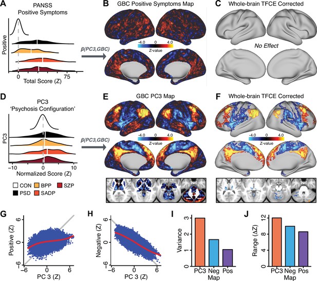
Dimensionality-reduced symptom variation reveals robust neurobehavioral mapping.

(A) Distributions of total PANSS Positive symptoms for each of the clinical diagnostic groups normalized relative to the control group (white = CON; black = all PSD patients; yellow = BPP; orange = SADP; red = SZP). (B) $β_{P o s i t i v e} G B C$ map showing the relationship between the aggregate PANSS Positive symptom score for each patient regressed onto global brain connectivity (GBC) across all patients (N = 436). (C) No regions survived non-parametric family-wise error (FWE) correction at p<0.05 using permutation testing with threshold-free cluster enhancement (TFCE). (D) Distributions of scores for *PC3 ‘Psychosis Configuration’* across clinical groups, again normalized to the control group. (E) $β_{P C 3} G B C$ map showing the relationship between the *PC3 ‘Psychosis Configuration’* score for each patient regressed onto GBC across all patients (N = 436). (F) Regions surviving p<0.05 FWE whole-brain correction via TFCE showed clear and robust effects. (G) Comparison between the *Psychosis Configuration* symptom score versus the aggregate PANSS Positive symptom score GBC map for every datapoint in the neural map (i.e. greyordinate in the CIFTI map). The sigmoidal pattern indicates an improvement in the Z-statistics for the *Psychosis Configuration* symptom score map (panel E) relative to the aggregate PANSS Positive symptom map (panel B). (H) A similar effect was observed when comparing the *Psychosis Configuration* GBC map relative to the PANSS Negative symptoms GBC map (Appendix 1—figure 8). (I) Comparison of the variances for the *Psychosis Configuration*, PANSS Negative and PANSS Positive symptom map Z-scores. (J) Comparison of the ranges between the *Psychosis Configuration*, Negative and Positive symptom map Z-scores. Symptom-neural maps for all five PCs and all four traditional symptom scales (BACS and PANSS subscales) are shown in Appendix 1—figure 8.

Figure 4

Download asset Open asset

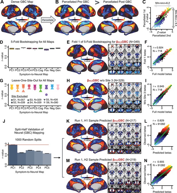
Parcellated symptom-neural GBC maps reflecting psychosis configuration are statistically robust and reproducible.

(A) Z-scored *PC3 Psychosis Configuration* GBC neural map at the ‘dense’ (full CIFTI resolution) level. (**B, C**) Neural data parcellated using a whole-brain functional partition (Ji et al., 2019b) *before* computing subject-level GBC yielded stronger statistical values in the Z-scored *Psychosis Configuration* GBC neural map as compared to when parcellation was performed *after* computing GBC for each subject. (D) Summary of similarities between all symptom-neural $β G B C$ maps (PCs and traditional symptom scales) across fivefold cross-validation. Boxplots show the range of r values between $β G B C$ maps for each fold and the full model. (E) Normalized $β G B C$ map from regression of individual patients’ *PC3* scores onto parcellated GBC data, shown here for a subset of patients from Fold 1 out of 5 (N = 349). The greater the magnitude of the coefficient for a parcel, the stronger the statistical relationship between GBC of that parcel and *PC3* score. (F) Correlation between the $β G B C$ value of each parcel in the regression model computed using patients in Fold one and the full PSD sample (N = 436) model indicates that the leave-one-fold-out $β G B C$ map was highly similar to the $β G B C$ map obtained from the full PSD sample model (r = 0.924). (G) Summary of leave-one-site-out regression for all symptom-neural maps. Regression of PC symptom scores onto parcellated GBC data, each time leaving out subjects from one site, resulted in highly similar maps. This highlights that the relationship between *PC3* scores and GBC is robust and not driven by a specific site. (H) $β G B C$ map for all PSD except one site. As an example, Site 3 is excluded here given that it recruited the most patients (and therefore may have the greatest statistical impact on the full model). (I) Correlation between the value of each parcel in the regression model computed using all patients minus Site 3, and the full PSD sample model. (J) Split-half replication of $β_{P C 3} G B C$ map. Bar plots show the mean correlation across 1000 runs; error bars show standard error. Note that the split-half effect for *PC1* was exceptionally robust. The split-half consistency for *PC3*, while lower, was still highly robust and well above chance. (K) $β_{P C 3} G B C$ map from *PC3*-to-GBC regression for the first half (H1) patients, shown here for one exemplar run out of 1000 split-half validations. (L) Correlation across 718 parcels between the H1 predicted coefficient map (i.e. panel K) and the observed coefficient map for H1. (**M–N**) The same analysis as K-L is shown for patients in H2, indicating a striking consistency in the *Psychosis Configuration* $β_{P C 3} G B C$ map correspondence.

Figure 5

Download asset Open asset

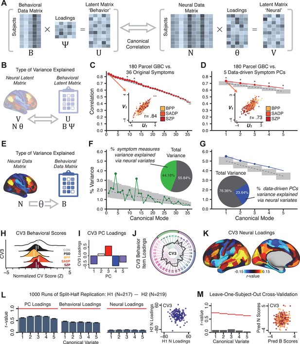
Multivariate symptom-neural feature mapping using canonical correlation analysis (CCA).

(A) Schematic of CCA data (**B, N**), transformation ( $Ψ$ , $Θ$ ), and transformed ‘latent’ (U, V) matrices. Here, each column in U and V is referred to as a canonical variate (CV); each corresponding pair of CVs (e.g. U₁ and V₁) is referred to as a canonical mode. (B) CCA maximized correlations between the CVs (U and V) (C) Screeplot showing canonical modes obtained from 180 neural features (cortical GBC symmetrized across hemispheres) and 36 symptom measures (‘180 vs. 36 CCA’). Inset illustrates the correlation (r = 0.85) between the CV of the first mode, U₁ and V₁ (note that the correlation was not driven by a separation between diagnoses). Modes 9 and 12 remained significant after FDR correction. (D) CCA computed with 180 neural features and five PC symptom features (‘180 vs. 5 CCA’). Here, all modes remained significant after FDR correction. Dashed black line shows the null calculated via a permutation test with 5000 shuffles; gray bars show 95% confidence interval. (E) Correlation between B and N $Θ$ reflects how much of the symptom variation can be explained by the latent neural features. (F) Proportion of symptom variance explained by each of the neural CVs in the 180 vs. 36 CCA. Inset shows the total proportion of behavioral variance explained by the neural CVs. (G) Proportion of total symptom variance explained by each of the neural CVs in the 180 vs. 5 CCA. While CCA using symptom PCs has fewer dimensions and thus accounts for lower total variance (see inset), each neural variate explains a higher amount of symptom variance than in F, suggesting that CCA could be optimized by first obtaining a low-rank symptom solution. Dashed black line indicates the null calculated via a permutation test with 5000 shuffles; gray bars show 95% confidence interval. Neural variance explained by symptom CVs are plotted in Appendix 1—figure 15. (H) Distributions of *CV3* scores from the 180 vs. 5 CCA are shown here as an example of characterizing CV configurations. Scores for all diagnostic groups are normalized to CON. Additionally, (I) symptom canonical factor loadings, (J) loadings of the original 36 symptom measures, and (K) neural canonical factor loadings for *CV3* are shown. (L) Within-sample CCA cross-validation appeared robust (see Appendix 1—figure 17). However, a split-half replication of the 180 vs. 5 CCA (using two independent non-overlapping samples) was not reliable. Bar plots show the mean correlation for each CV between the first half (H1) and the second half (H2) CCA, each computed across 1000 runs. *Left:* split-half replication of the symptom PC loadings matrix $Ψ$ ; *Middle:* individual symptom measure loadings; *Right:* the neural loadings matrix $Θ$ , which in particular was not stable. Error bars show the standard error of the mean. Scatterplot shows the correlation between *CV3* neural loadings for H1 vs. H2 for one example CCA run, illustrating lack of reliability. (M) Leave-one-subject-out cross-validation further highlights CCA instability.

Figure 6

Download asset Open asset

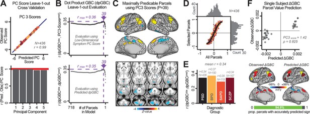
Optimizing neural feature selection to inform single-subject prediction via a low-dimensional symptom solution.

(A) Leave-one-out cross-validation for the symptom PCA analyses indicates robust individual score prediction. Top panel: Scatterplot shows the correlation between each subject's predicted *PC3* score from a leave-one-out PCA model and their observed *PC3* score from the full-sample PCA model, r = 0.99. Bottom panel: Correlation between predicted and observed individual PC scores was above 0.99 for each of the significant PCs (see Figure 1). The red line indicates r = 1. (B) We developed a univariate step-down feature selection framework to obtain the most predictive parcels using a subject-specific approach via the $d p G B C$ index. Specifically, the ’observed’ patient-specific $d p G B C^{o b s}$ was calculated using each patient’s $Δ G B C^{o b s}$ (i.e. the patient-specific GBC map vs. the group mean GBC for each each parcel) and the ‘reference’ symptom-to-GBC *PC3* map (described in Figure 4B) [ $d p G B C^{o b s}$ = $Δ G B C^{o b s} \cdot β_{P C 3} G B C^{o b s}$ ]. See **Materials and methods** and Appendix 1—figure 24 for complete feature selection procedure details. In turn, we computed the predicted $d p G B C$ index for each patient by holding their data out of the model and predicting their score ( $d p G B C^{p r e d}$ ). We used two metrics to evaluate the maximally predictive feature subset: (i) The correlation between *PC3* symptom score and $d p G B C^{o b s}$ across all N = 436, which was maximal for $P = 39$ parcels [r = 0.36, purple arrow]; (ii) The correlation between $d p G B C^{o b s}$ and $d p G B C^{p r e d}$ , which also peaked at $P = 39$ parcels [r = 0.35, purple arrow]. (C) The $P = 39$ maximally predictive parcels from the $β_{P C 3} G B C^{o b s}$ map are highlighted (referred to as the ‘selected’ map). (D) Across all n = 436 patients we evaluated if the selected parcels improve the statistical range of similarities between the $Δ G B C^{o b s}$ and the $β_{P C 3} G B C^{o b s}$ reference for each patient. For each subject the value on the X-axis reflects a correlation between their $Δ G B C^{o b s}$ map and the $β_{P C 3} G B C^{o b s}$ map across all 718 parcels; the Y-axis reflects a correlation between their $Δ G B C^{o b s}$ map and the $β_{P C 3} G B C^{o b s}$ map only within the ‘selected’ 39 parcels. The marginal histograms show the distribution of these values across subjects. (E) Each DSM diagnostic group showed comparable correlations between predicted and observed $d p G B C$ values. The r-value shown for each group is a correlation between the $d p G B C^{o b s}$ and $d p G B C^{p r e d}$ vectors, each of length N. (F) Scatterplot for a single patient with a positive behavioral loading ( $P C 3$ score = 1.42) and also with a high correlation between predicted $Δ G B C^{p r e d}$ versus observed $Δ G B C^{o b s}$ values for the ‘selected’ 39 parcels ( $ρ = 0.825$ ). Right panel highlights the observed vs. predicted $Δ G B C$ map for this patient, indicating that 94.9% of the parcels were predicted in the correct direction (i.e. in the correct quadrant).

Figure 7

Download asset Open asset

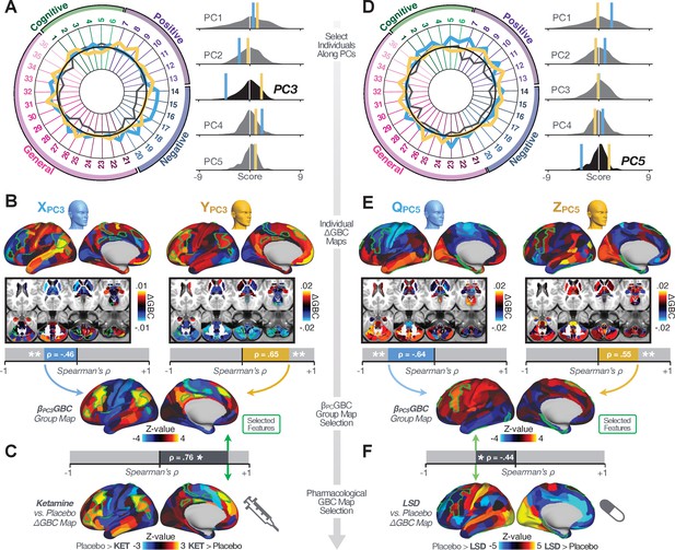
Leveraging subject-specific brain-behavioral maps for molecular neuroimaging target selection.

(A) Data for two individual patients from the replication dataset are highlighted for PC3: $X_{P C 3}$ (blue) and $Y_{P C 3}$ (yellow). Both of these patients scored above the neural and behavioral thresholds for *PC3* defined in the ‘discovery’ PSD dataset. Patient $X_{P C 3}$ loads highly negatively on the *PC5* axis and Patient $Y_{P C 3}$ loads highly positively. Density plots show the projected PC scores for Patients $X_{P C 3}$ and $Y_{P C 3}$ overlaid on distributions of PC scores from the discovery PSD sample. (B) Neural maps show cortical and subcortical $Δ G B C^{o b s}$ for the two patients $X_{P C 3}$ and $Y_{P C 3}$ specifically reflecting a difference from the mean *PC3*. The similarity of $Δ G B C^{o b s}$ and the $β_{P C 3} G B C^{o b s}$ map within the most predictive neural parcels for PC3 (outlined in green). Note that the sign of neural similarity to the reference *PC3* map and the sign of the *PC3* score is consistent for these two patients. (C) The selected *PC3* map (parcels outlined in green) is spatially correlated to the neural map reflecting the change in GBC after ketamine administration (ρ = 0.76, **Materials and methods**). Note that Patient $X_{P C 3}$ who exhibits $Δ G B C^{o b s}$ that is anti-correlated to the ketamine map also expresses depressive moods symptoms (panel A). This is consistent with the possibility that this person may clinically benefit from ketamine administration, which may elevate connectivity in areas where they show reductions (Berman et al., 2000). In contrast, Patient $Y_{P C 3}$ may exhibit an exacerbation of their psychosis symptoms given that their $Δ G B C^{o b s}$ is positively correlation with the ketamine map. (D) Data for two individual patients from the discovery dataset are highlighted for PC5: $Q_{P C 5}$ (blue) and $Z_{P C 5}$ (yellow). Note that no patients in the replication dataset were selected for *PC5* so both of these patients were selected from ‘discovery’ PSD dataset for illustrative purposes. Patient $Q_{P C 5}$ loads highly negatively on the *PC5* axis and Patient $Z_{P C 5}$ loads highly positively. Density plots show the projected PC scores for Patients $Q_{P C 5}$ and $Z_{P C 5}$ overlaid on distributions of PC scores from the discovery PSD sample. (E) Neural maps show cortical and subcortical $Δ G B C^{o b s}$ for Patients $Q_{P C 5}$ and $Z_{P C 5}$ , which are highly negatively and positively correlated with the selected *PC5* map respectively. (F) The selected *PC5* map (parcels outlined in green) is spatially anti-correlated with the LSD response map (ρ = −0.44, see **Materials and methods**), suggesting that circuits modulated by LSD (i.e. serotonin, in particular 5-HT2A) may be relevant for the *PC5* symptom expression. Here, a serotonin receptor agonist may modulate the symptom-neural profile of Patient $Q_{P C 5}$ , whereas an antagonist may be effective for Patient $Z_{P C 5}$ .

Figure 8

Download asset Open asset

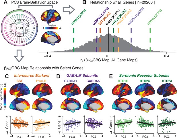
Psychosis spectrum symptom-neural maps track neural gene expression patterns computed from the Allen Human Brain Atlas (AHBA).

(A) The symptom loadings and the associated neural map jointly reflect the *PC3* brain-behavioral space (BBS) profile, which can be quantitatively related to human cortical gene expression patterns obtained from the AHBA (Burt et al., 2018). (B) Distribution of correlation values between the *PC3* BBS map and ∼20,000 gene expression maps derived from the AHBA dataset. Specifically, AHBA gene expression maps were obtained using DNA microarrays from six postmortem brains, capturing gene expression topography across cortical areas. These expression patterns were then mapped onto the cortical surface models derived from the AHBA subjects’ anatomical scans and aligned with the Human Connectome Project (HCP) atlas, described in prior work and methods (Burt et al., 2018). Note that because no significant inter-hemispheric differences were found in cortical gene expression all results were symmetrized to the left hemisphere, resulting in 180 parcels. We focused on a select number of psychosis-relevant genes – namely genes coding for the serotonin and GABA receptor subunits and interneuron markers. Seven genes of interest are highlighted with dashed lines. Note that the expression pattern of HTR2C (green dashed line) is at the low negative tail of the entire distribution, that is highly anti-correlated with *PC3* BBS map. Conversely, GABRA1 and HTR1E are on the far positive end, reflecting a highly similar gene-to-BBS spatial pattern. (C) Upper panels show gene expression patterns for two interneuron marker genes, somatostatin (SST) and parvalbumin (PVALB). Positive (yellow) regions show areas where the gene of interest is highly expressed, whereas negative (blue) regions indicate low expression values. Lower panels highlight all gene-to-BBS map spatial correlations where each value is a symmetrized cortical parcel (180 in total) from the HCP atlas parcellation. (D) Gene expression maps and spatial correlations with the *PC3* BBS map for two GABA_A receptor subunit genes: GABRA1 and GABRA5. (E) Gene expression maps and spatial correlations with the *PC3* BBS map for three serotonin receptor subunit genes: HTR1E, HTR2C, and HTR2A.

Appendix 1—figure 1

Download asset Open asset

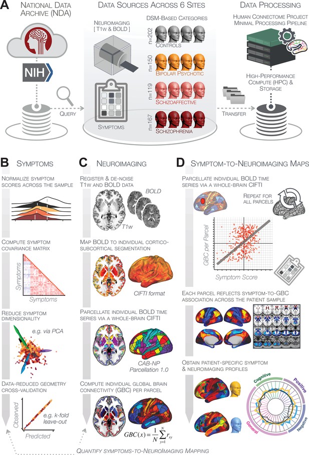
Study workflow used study to quantify shared neural and behavioral variation in individuals diagnosed with PSD.

(A) Data from the BSNIP study were acquired from the National Institute of Health Data Archive (NDA). T1-weighted structural and resting-state BOLD neuroimaging data were obtained for a total of 638 individuals (202 controls, 150 patients with a diagnosis of bipolar disorder with psychosis, 119 with a diagnosis of schizoaffective disorder, and 167 patients with schizophrenia). Data were processed through the Human Connectome Project’s (HCP) Minimal Preprocessing Pipeline with modifications made for ‘legacy’ BOLD and T1w data, which are now featured as a standard option in the HCP pipelines provided by our team (https://github.com/Washington-University/HCPpipelines/pull/156) using Yale High Performance Computing clusters. (B) Symptom data were first normalized across the sample. The correlation matrix across all 436 PSD patients and 36 symptom measures was computed followed by dimensionality reduction (e.g. using PCA or ICA). The dimensionality-reduced solution was then cross-validated to assess stability and reproducibility across sites, k-fold cross-validations, leave-subject-out and split-half approaches. (C) In parallel, all neuroimaging data were processed as noted above. T1w and resting-state BOLD images were preprocessed using a modified version of the HCP Minimal Preprocessing Pipeline, including individual-subject registration of structural and function data, de-noising, and mapping of BOLD data on a hybrid surface-volume cortico-subcortical format (Connectivity Informatics Technology Initiative [CIFTI] format, see **Materials and methods** for details). After registration to a standard CIFTI template BOLD data were parcellated at the individual subject level using the Cole-Anticevic Brain-wide Network Partition (CAB-NP), which is a functionally-defined network and parcel-level partition in the CIFTI space encompassing both cortex and subcortex (Glasser et al., 2016; Ji et al., 2019b). Lastly, a global brain connectivity (GBC) map for each subject was computed by taking the mean functional connectivity of each parcel with all other parcels in the brain at the single subject level. (D) After symptom and neural data were fully processed in tandem, the symptom-to-neuroimaging mapping was quantified across subjects. Specifically, the relationship between data-reduced symptom scores and GBC was computed for each parcel across all patients. This produced a group-level symptom-neural map, which was subsequently cross-validated using leave-site-out, k-fold, leave subject-out as well as split-half approaches to assess reproducibility of the effect. Finally, the stable symptom-neural mapping result was further feature-optimized for single-subject prediction. This yielded a set of parcels for quantifying patient-specific symptom-neural prediction based on a cross-validated group reference map as well as comparison of the selected parcels with independent molecular neuroimaging maps (i.e. pharmacological [Anticevic et al., 2012a; Preller et al., 2018] and gene expression maps [Burt et al., 2018]).

Appendix 1—figure 2

Download asset Open asset

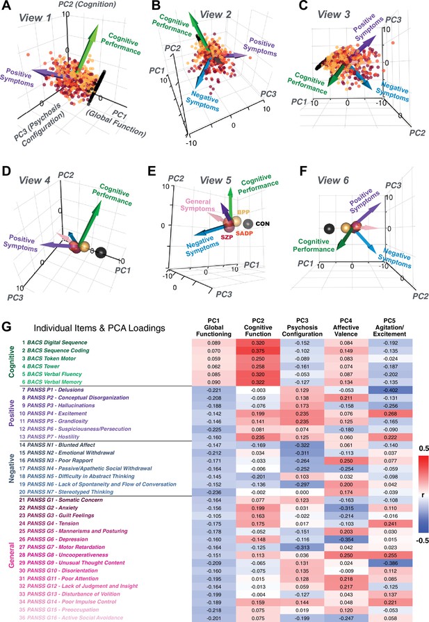
Alternative views of the behavioral PCA triplot.

(**A–C**) Alternative views of the triplot in Figure 1F showing the relationship between the three principal axes of variation in behavior and standard clinical symptom factors. Each point represents an individual subject projected into the geometry defined by the first three principal components (PC). Vectors show the projections of standard symptoms factors. (**D–F**) Alternative views of the triplot in panels A–C, where each sphere represents the mean of each a priori clinical group. Vectors show the projections of standard symptoms factors [PANSS positive (purple), negative (blue), general (pink) symptoms and BACS cognitive performance (green)]. BPP, bipolar disorder; SADP, schizoaffective disorder; SZP, schizophrenia; CON, controls. (G) Heatmap of the loadings of each of the 36 symptom measures on the five significant PCs (also seen in radarplot in Figure 1E). Positive loadings are indicated in red; negative loadings are shown in blue. Each PC is named based on its most strongly loaded items.

Appendix 1—figure 3

Download asset Open asset

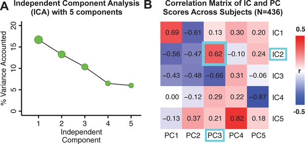
Independent component analysis (ICA) as an alternative method of dimensionality-reduction of symptom data.

(A) Screeplot showing the total proportion of variance explained by each independent component (IC) in a five-component solution performed across all 36 behavioral measures in 436 patients. The size of each point is proportional to the variance explained by that IC. (B) Correlation matrix showing correlations of individual subject scores for the five significant principal components (PCs) from the PCA solution shown in Figure 1 and the five ICs from the ICA solution, across all 436 subjects. Neural maps for each IC are shown in Appendix 1—figure 12.

Appendix 1—figure 4

Download asset Open asset

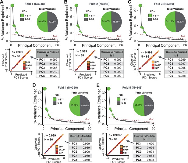
k-Fold cross-validation for symptom-driven principal component analysis (PCA).

These results show a fivefold cross-validation analysis to test the stability of the PCA solution. The full patient sample was first randomly split into five sets and patients were randomly assigned to one of five subsets. Each subset of patients was then used as an independent ‘test sample’ in a PCA that was derived from the other four subsets. Screeplot shows proportion of variance explained by each of the PCs in a PCA of all 36 behavioral measures, excluding a subset of 88 patients. The number of significant PCs determined via a permutation test and the total proportion of variance explained by these PCs are all comparable to the full model shown in the main text. To obtain a ‘predicted’ PC score for the 88 patients in the excluded subset, the loadings from the model obtained from the other 348 patients were used. The ‘observed’ PC scores are the scores from the full model of the same 88 patients. The scatterplot shows that the predicted and observed scores for *PC1* are highly correlated (r = 0.999), suggesting that the PCA solution is stable and predictive at the individual-subject level. Similarly, predicted and observed scores are highly correlated for all five PCs. (**B–E**) The results of the PCA are also highly comparable and predictive for the other four folds.

Appendix 1—figure 5

Download asset Open asset

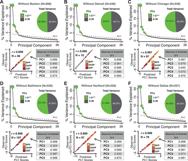
Leave-site-out cross-validation for symptom-driven principal component analysis (PCA).

These results show a sixfold leave-site-out cross-validation analysis to test the stability of the PCA solution when a given site is excluded from the model. The full patient sample was first split into six sets according to data collection site. Each held-out site was then used as an independent ‘test sample’ in a PCA that was derived from the other five sites. (A) Proportion of variance explained by each of the PCs in a PCA of all 36 behavioral measures, excluding one of the six sites at which data was collected (here we excluded the Boston site). The number of significant PCs determined via a permutation test and the total proportion of variance explained by these PCs are all comparable to the full model shown in Figure 1C. To obtain a ‘predicted’ PC score for the 46 patients in the excluded site, the loadings from the model obtained from the other 390 patients were used. The ‘observed’ PC scores are the scores from the full model of the same 88 patients. The scatterplot shows that the predicted and observed scores for *PC1* are highly correlated (r = 0.999), suggesting that the PCA solution is stable and robustly predictive at the individual patient level. Predicted and observed scores are highly correlated for all five PCs. (**B–F**) The results of the PCA are also highly comparable for the other five sites, suggesting that possible site differences in evaluating patient symptoms or patient sample composition are not impacting the obtained PCA solutions.

Appendix 1—figure 6

Download asset Open asset

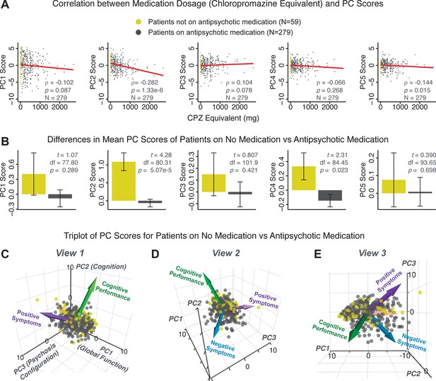
PCA solution is not driven by medication status or dosage.

Antipsychotic medication dosages were available for N = 338 out of 436 PSD patients, including 59 patients not on antipsychotic medication. Antipsychotic dosages were converted to chlorpromazine (CPZ) equivalents (Lencer et al., 2015). (A) Spearman’s ρ between medication dosage (CPZ equivalents) and PC scores for each of the five significant principal components (PCs), for medicated patients (gray points). Patients not on antipsychotic medication are also shown (yellow points, CPZ = 0 mg); however, they were not included in the calculation of Spearman’s ρ as they contain no rank information. (B) Bar plots show the mean PC scores of unmedicated (yellow) versus medicated (gray) PSD patients for each of the five PCs. Error bars show standard error of the mean. Note that only PC2 ‘Cognitive Performance’ scores appear to show a significant relationship with medication consistently; this could be because antipsychotic medication (particularly first-generation antipsychotics) are related to symptom variance across some PCA-derived symptom dimensions but do not effectively treat cognitive deficits. Also, cognitive deficits (such as reaction time and fluency) may be exacerbated due to the neuroleptic effects of first-generation antipsychotics. (**C–E**) Alternative views of the triplot (as seen in Appendix 1—figure 2A–C) showing the relationship between the three principal axes of variation in symptoms and aggregate scores from the PANSS and BACS symptom scales (i.e. vectors show the projections of standard symptoms factors). Each point represents an individual patient projected into the geometry defined by the first three principal components (PC). Each patient is colored according to medication status (yellow = unmedicated, gray = with medication). As evident from this plot there is no apparent clustering of patients according to their medication status in the 3D PCA-derived space.

Appendix 1—figure 7

Download asset Open asset

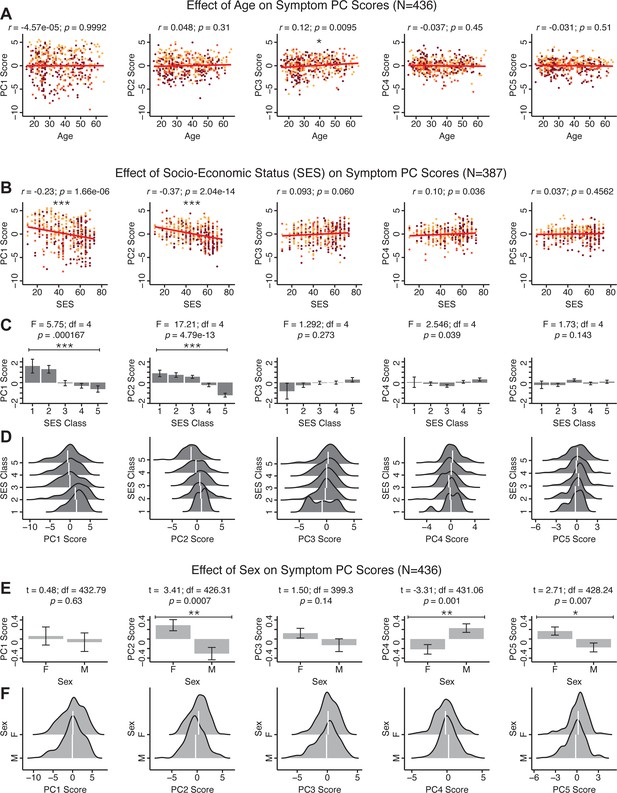
Effects of age, socio-economic status, and sex on symptom PCA solution.

(A) Correlations between symptom PC scores and age (years) across N = 436 PSD. Pearson’s correlation value and uncorrected p-values are reported above scatterplots. After Bonferroni correction, we observed a significant positive relationship between age and *PC3* score. This may be because older patients have been ill for a longer period of time and exhibit more severe symptoms along the positive *PC3* dimension. (B) Correlations between symptom PC scores and socio-economic status (SES) as measured by the Hollingshead Index of Social Position (Hollingshead, 1975), across N = 387 PSD with available data. The index is computed as (Hollingshead occupation score * 7) + (Hollingshead education score * 4); a higher score indicates lower SES (Padmanabhan et al., 2015). We observed a significant negative relationship between Hollingshead index and *PC1* and PC2 scores. Lower *PC1* and *PC2* scores indicate poorer general functioning and cognitive performance respectively, which is consistent with higher Hollingshead indices (i.e. lower-skilled jobs or unemployment and fewer years of education). (C) The Hollingshead index can be split into five classes, with one being the highest and five being the lowest SES class (Hollingshead, 1975). Consistent with (B) we found a significant difference between the classes after Bonferroni correction for *PC1* and *PC2* scores. (D) Distributions of PC scores across Hollingshead SES classes show the overlap in scores. White lines indicate the mean score in each class. (E) Differences in PC scores between (M)ale and (F)emale PSD subjects. We found a significant difference between sexes in *PC2 – Cognitive Functioning*, *PC4 – Affective Valence*, and *PC5 – Agitation/Excitement* scores. (F) Distributions of PC scores across M and F subjects show the overlap in scores. White lines indicate the mean score for each sex.

Appendix 1—figure 8

Download asset Open asset

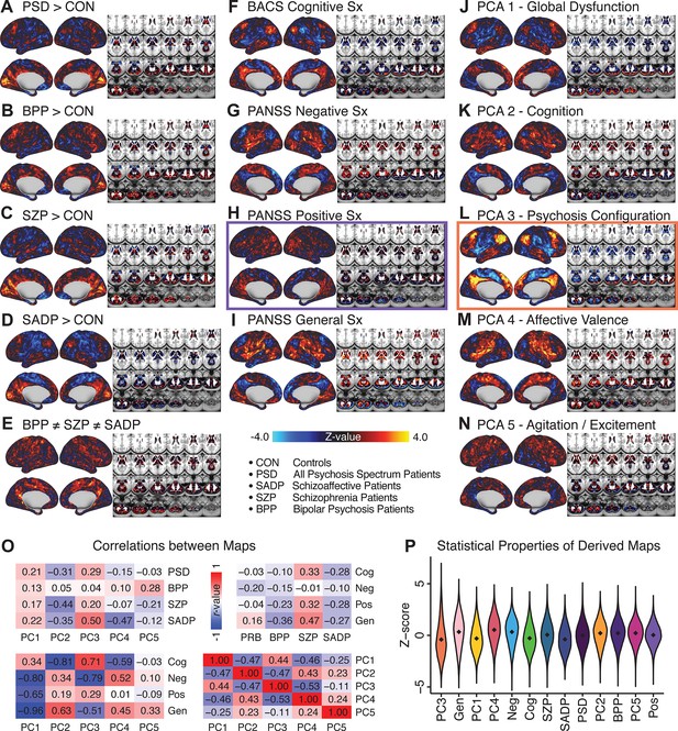
Similarity across a priori, categorical and PCA-derived brain-behavioral GBC maps.

Z-scored maps of t-test for the difference in group mean GBC between traditional diagnostic groups: (A) all patients (PSD) versus all healthy controls (CON); (B) patients with bipolar disorder (BPP) versus CON; (C) patients with schizophrenia (SZP) versus CON; (D) patients with schizoaffective disorder (SADP) versus CON. (E) Z-scored map of the F-test for the difference in group mean GBC between patients in all three diagnostic groups (BPP, SZP, SADP). Z-scored map of the regression against GBC, across all patients (PSD), of traditional symptom/behavioral scales: (F) BACS cognitive composite performance score; (G) PANSS total negative symptom score; (H) PANSS total positive symptom score; (I) PANSS total general symptom score. Z-scored map of the regression against GBC, across all patients, of data-derived behavioral dimension scores: (J) *PC1* score; (K) PC2 score; (L) *PC3* score; (M) *PC4* score; (N) *PC5* score. (O) Correlation matrices showing the similarity between brain-behavioral maps in A-N. (P) Violin plots of the distribution of Z-values in all phenotype maps. Note that although there are strong correlations between the PC maps and the a priori symptom maps, the statistical properties of some of the PC maps are improved (i.e. the range of Z-scores is greater, with more extreme values), suggesting a stronger mapping between neural and behavioral variation.

Appendix 1—figure 9

Download asset Open asset

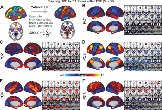
Parcellated symptom-neural GBC maps across all PSD patients derived from PCA dimensionality reduction of symptom measures.

(A) All of the maps shown here were parcellated at the single patient level using the Cole-Anticevic Brain Network Parcellation (CAB-NP) parcellation (Ji et al., 2019b), which defines functional networks and regions across cortex and subcortex that leveraged the Human Connectome Project's Multi-Modal Parcellation (MMP1.0) (Glasser et al., 2016; Ji et al., 2019b). The final published CAB-NP 1.0 parcellation solution can be visualized via the Brain Analysis Library of Spatial maps and Atlases (BALSA) resource (https://balsa.wustl.edu/rrg5v) and downloaded from the public repository (https://github.com/ColeLab/ColeAnticevicNetPartition). (**B–F**) Relationships across all patients (N = 436) at each parcel location between global brain connectivity (GBC) and PC score for each of the significant PCs. Values shown in each brain parcel is the Z-scored regression coefficient of PC score on to parcel GBC, across all 436 subjects.

Appendix 1—figure 10

Download asset Open asset

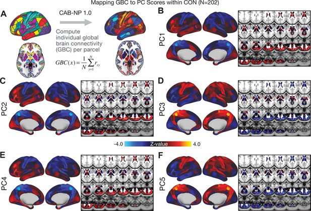
Parcellated symptom-neural GBC maps across all CON subjects derived from PCA dimensionality reduction of PSD symptom measures.

(A) As with PSD maps, all of the maps shown here were parcellated at the single patient level using the Cole-Anticevic Brain Network Parcellation (CAB-NP) parcellation (Ji et al., 2019b), which defines functional networks and regions across cortex and subcortex that leveraged the Human Connectome Project's Multi-Modal Parcellation (MMP1.0) (Glasser et al., 2016; Ji et al., 2019b). The final published CAB-NP 1.0 parcellation solution can be visualized via the Brain Analysis Library of Spatial maps and Atlases (BALSA) resource (https://balsa.wustl.edu/rrg5v) and downloaded from the public repository (https://github.com/ColeLab/ColeAnticevicNetPartition). (**B–F**) Relationships across all controls (N = 202) at each parcel location between global brain connectivity (GBC) and PC score for each of the significant PCs. Values shown in each brain parcel is the Z-scored regression coefficient of PC score on to parcel GBC, across all 202 control subjects.

Appendix 1—figure 11

Download asset Open asset

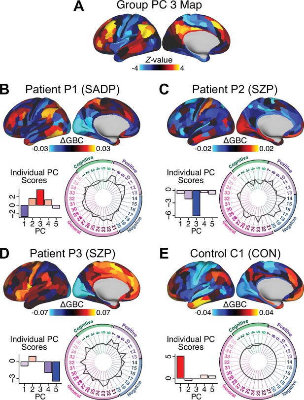
Individual patients exhibit complex projections into the PCA-derived brain-behavioral space (BBS) geometry (A) The *PC3* group-level cortical map is shown here for comparison purposes.

(B) Neural and behavioral profile for one PSD patients, ‘Patient P1’. Neural data shows the ΔGBC for Patient P1 (i.e. GBC demeaned relative to group mean of the entire PSD patient sample) to reflect the pattern of changes in their GBC relative to the ’average’ of the entire sample. The bar plot shows five behavioral PC scores for Patient P1. The radarplot shows original scores on the 36 individual symptom measures for Patient P1 (black circle indicates zero; positive values are indicated by outward deviation of the gray line). (C–D) Data is shown for two other individual Patients P2 and P3. (E). Data is shown for one Control C1 participant. Note the difference between the symptom-neural profiles of Patient P1, a positive *PC3* ‘loading’ individual, and Patient P2, a negative *PC3* ’loading’ individual, both of whom were diagnosed with SZP under a conventional categorical DSM approach. These data further illustrate the need to consider the complex relationships in the symptom-neural mapping and highlight that individual-level precision in BBS mapping can be obtained.

Appendix 1—figure 12

Download asset Open asset

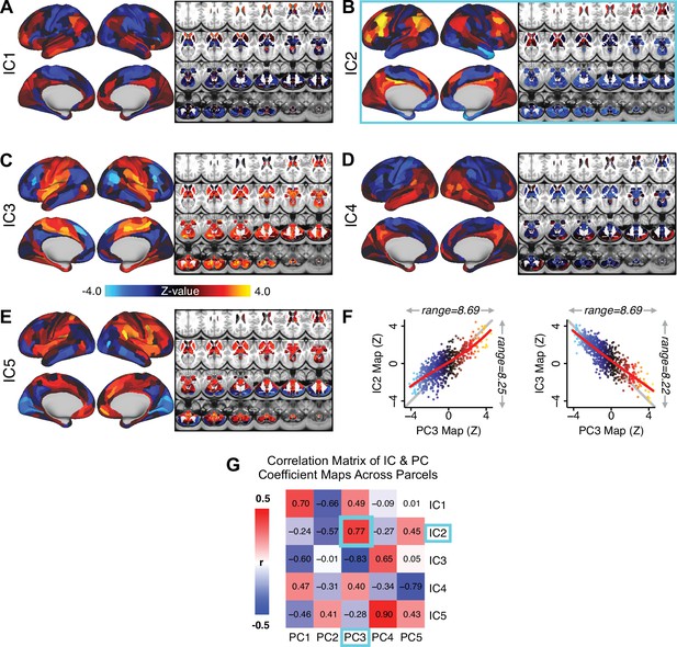
Independent component analysis (ICA) as an alternative method of dimensionality-reduction for symptom-neural mapping.

(**A–E**) Relationships across all patients (N = 436) at each brain location between global brain connectivity (GBC) and IC score, for ICs 1–5. Values shown in each brain parcel is the Z-scored regression coefficient of IC score on to parcel GBC, across all 436 subjects. (F) Scatterplots showing the relationships across parcels between the PC3 map and the IC2 and IC3 maps. Sigmoids and a greater range (max - min) indicate an improvement in the Z-statistics of the PC3 map relative to the IC maps. (G) Correlation matrix showing correlations of individual parcel regression coefficients for the five significant PCs and the five ICs (shown in A–E), across all 718 neural parcels. Of note, *PC3 ‘Psychosis Configuration’* discovered via the PCA solution appears to be oblique to both *IC2* and *IC3*, suggesting that these two *ICs* may capture diverging tails of the *PC3* axis; however, the orthogonality of the PCA solution yielded maximally separated symptom dimensions that mapped on to unique neural variance, as shown by the superior statistics of the PC3 map versus the *IC2/IC3* maps.

Appendix 1—figure 13

Download asset Open asset

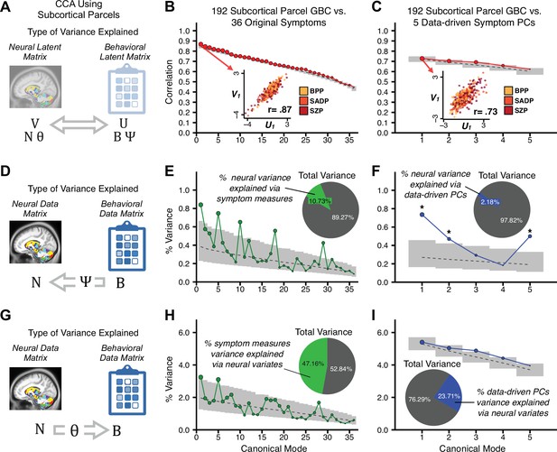
Canonical correlation analysis (CCA) of behavioral and subcortical neural features.

(A) As noted in the main text, CCA maximizes correlations between canonical variates (CVs), that is matrices U and V. Here we evaluated a version of CCA using subcortical neural parcel features in relation to item-level symptom measures or dimensionality-reduced PC symptom measures. (B) Screeplot showing canonical modes for the CVs obtained from 192 subcortical neural features (GBC of parcels from a neurobiologically-derived functional parcellation of the subcortex) and 36 single-item PANSS and BACS symptom measures. Inset illustrates the correlation (r = 0.85) between the CV of the first mode, U₁ and V₁ (note that the correlation was not driven by a separation between diagnoses). (C) CCA was obtained from 192 subcortical neural features and five low-dimensional symptom scores derived via the PCA analysis. Here, all modes remained significant after FDR correction. Dashed black line shows the null calculated via a permutation test with 5000 shuffles; gray bars show 95% confidence interval. (D) Correlation between the neural data matrix N and the behavioral data matrix weighted by the transformation matrix (BΨ) reflects the amount of variance in N that can be explained by the final latent neural matrix U. Put differently, this transformation calculates how much of the neural variation can be explained by the latent behavioral features. (E) Proportion of symptom variance explained by each of the neural CVs in a CCA performed between 192 subcortical neural features and all 36 behavioral measures. Inset shows the total proportion of behavioral variance explained by the neural variates. (F) Proportion of total behavioral variance explained by each of the neural CVs in a CCA performed between 192 subcortical neural features and the five low-dimensional symptom scores derived via the PCA analysis. Dashed black line shows the null calculated via a permutation test with 5000 shuffles; gray bars show 95% confidence interval. (G) Correlation between the behavioral data matrix B and the neural data matrix weighted by the transformation matrix (NΘ) reflects the amount of variance in B that can be explained by the final latent neural matrix V. Put differently, this transformation calculates how much of the symptom variation can be explained by the latent neural features. (H) Proportion of symptom variance explained by each of the neural CVs in a CCA performed between 192 subcortical neural features and all 36 behavioral measures. Inset shows the total proportion of behavioral variance explained by the neural variates. (I) Proportion of total behavioral variance explained by each of the neural CVs in a CCA performed between 192 subcortical neural features and the five low-dimensional symptom scores derived via the PCA analysis. While CCA using symptom PCs has fewer dimensions and thus lower total variance explained (see inset), each neural variate explains a higher amount of symptom variance than seen in F, suggesting that CCA could be further optimized by first obtained a principled low-rank symptom solution. Dashed black line shows the null calculated via a permutation test with 5000 shuffles; gray bars show 95% confidence interval.

Appendix 1—figure 14

Download asset Open asset

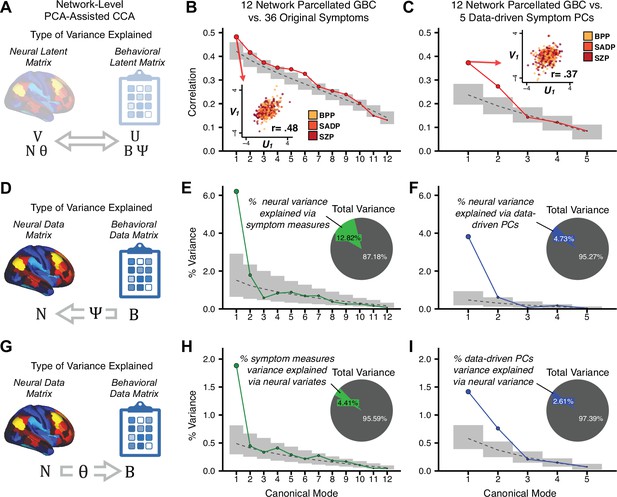
Canonical correlation analysis (CCA) of behavioral and network-level neural features.

(A) As noted in the main text, CCA maximizes correlations between canonical variates (CVs), that is matrices U and V. Here we evaluated a version of CCA using network-level neural parcel features in relation to item-level symptom measures or dimensionality-reduced PC symptom measures. (B) Screenplot showing canonical modes for the CVs obtained from 192 subcortical neural features (GBC of parcels from a neurobiologically derived functional parcellation of the subcortex) and 36 single-item PANSS and BACS symptom measures. Inset illustrates the correlation (r = 0.85) between the CV of the first mode, U₁ and V₁ (note that the correlation was not driven by a separation between diagnoses). (C) CCA was obtained from 192 subcortical neural features and five low-dimensional symptom scores derived via the PCA analysis. Here, all modes remained significant after FDR correction. Dashed black line shows the null calculated via a permutation test with 5000 shuffles; gray bars show 95% confidence interval. (B) Screeplot showing the correlations between the canonical variates of a CCA performed between 12 neural features (mean GBC of 12 whole-brain networks) and all 36 behavioral measures. Dashed black line shows the null calculated via a permutation test with 5000 shuffles; gray bars show 95% confidence interval. Inset illustrates the correlation (r = 0.48) between the canonical variates of the first mode, U₁ and V₁. Note that the correlation is not driven by a separation between categorical diagnoses. (C) Screeplot showing the correlations between the canonical variates of a CCA performed between 12 network neural features and the five behavioral principal components. Dashed black line shows the null calculated via a permutation test with 5000 shuffles; gray bars show 95% confidence interval. Inset illustrates the correlation (r = 0.37) between the canonical variates of the first mode, V₁ and V₁. Note that the strength of the correlations is greatly reduced compared to the parcel-level CCA shown in Figure 5. (D) The correlation between the neural data N and the transformed behavioral data matrix Bψ reflects the amount of variance in N that can be explained by behavioral canonical variates V. (E) Screeplot showing the proportion of neural variance explained by each of the behavioral canonical variates in a CCA performed between 12 network neural features and all 36 behavioral measures. Dashed black line shows the null calculated via a permutation test with 5000 shuffles; gray bars show 95% confidence interval. Inset shows the total proportion of neural variance explained by the behavioral variates. (F) Screeplot of the proportion of neural variance explained by each of the behavioral canonical variates in a CCA performed between 12 network neural features and the five PCs of behavior. (G) The correlation between the behavioral data B and the transformed neural data matrix NΘ reflects the amount of variance in B that can be explained by neural canonical variates U. (H) Screeplot showing the proportion of behavioral variance explained by each of the neural canonical variates in a CCA performed between 12 network neural features and all 36 behavioral measures. Dashed black line shows the null calculated via a permutation test with 5000 shuffles; gray bars show 95% confidence interval. Inset shows the total proportion of behavioral variance explained by the neural variates.t (I) Screeplot of the proportion of total behavioral variance explained by each of the neural canonical variates in a CCA performed between 12 network neural features and the 5 PCs of behavior. Note that although the CCA using behavioral PCs has far fewer dimensions, each neural variate explains a higher amount of total behavioral variance than neural variates in H, suggesting that the identified PCs of behavior capture variance with far fewer features.

Appendix 1—figure 15

Download asset Open asset

Canonical correlation analysis (CCA) results showing the amount of variance explained in the neural features via behavioral canonical variates.

(A) The correlation between the neural data N and the transformed behavioral data matrix Bψ reflects the amount of variance in N that can be explained by behavioral canonical variates. (B) Screeplot showing the proportion of neural variance explained by each of the behavioral canonical variates in a CCA performed between 180 neural features (symmetrized cortical parcel GBC) and all 36 behavioral measures. Dashed black line shows the null calculated via a permutation test with 5000 shuffles; gray bars show 95% confidence interval. Inset shows the total proportion of neural variance explained by the behavioral variates. (C) Screeplot of the proportion of neural variance explained by each of the behavioral canonical variates in a CCA performed between 180 neural features (symmetrized cortical parcel GBC) and the five PCs of behavior.

Appendix 1—figure 16

Download asset Open asset

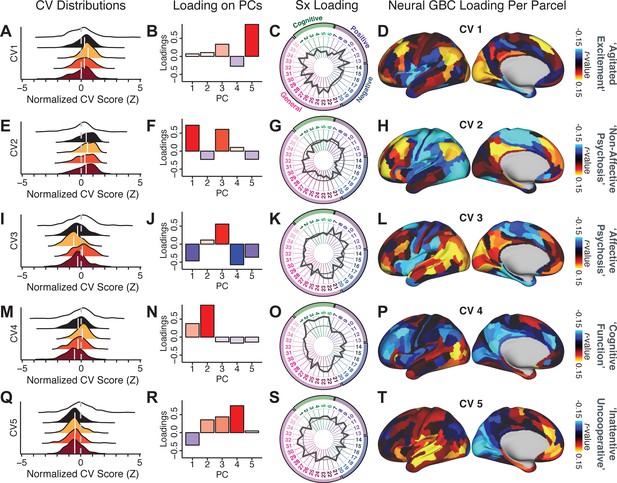
Canonical correlation analysis (CCA) symptom and neural configurations.

(A) Distributions of scores for the first canonical variate (*CV1*) by diagnostic group (white: controls; black: all patients; yellow: bipolar disorder with psychosis; orange: schizoaffective disorder with psychosis; red: schizophrenia). All scores are normalized to controls. (B) Loadings of the PC-derived symptom scores for *CV1*. (C) Loadings of the original item-level symptom measures for *CV1*. (D) Loadings of each neural parcel for *CV1*. (**E–T**) The same analyses are shown for canonical variates 2–5. As noted in the main text, these CCA effects were not stable when tested via out-of-sample cross-validation methods (see Figure 5).

Appendix 1—figure 17

Download asset Open asset

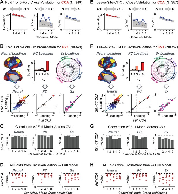
K-Fold cross-validation of canonical correlation analysis (CCA).

In the main text, we show that CCA effects do not reproduce when tested via out-of-sample cross-validation methods (see Figure 5). In contrast, here we show that using within-sample K-fold methods yields effects that appear reproducible but in fact reflect an overfit CCA solution. Panels (**A–E**) illustrate the results from a 5-fold cross-validation analysis to test the reproducibility of the CCA solution. Subjects were first randomly assigned to one of five subsets. Each subset of subjects was then used as an independent ‘test sample' in a CCA that was derived from subjects in the other four subsets. (A) Results of CCA performed in a subsample of N = 349 subjects. Left: screeplot showing the correlations between the canonical variates of a CCA performed between 180 neural features (symmetrized cortical parcel GBC) and the five behavioral principal components in N = 349 subjects. Middle: Screeplot of the proportion of neural variance explained by each of the behavioral canonical variates in a CCA performed between 180 neural features (symmetrized cortical parcel GBC) and the five PCs of behavior. Right: Screeplot of the proportion of total behavioral variance explained by each of the neural canonical variates in a CCA performed between 180 neural features (symmetrized cortical parcel GBC) and the five PCs of behavior. Dashed black line shows the null calculated via a permutation test with 5000 shuffles; gray bars show 95% confidence interval. Note that the outcome of this CCA is highly similar to the full sample CCA shown in the main text, but it is not similar at all to the split-half cross-validation effects, which reveal how overfit CCA effects seem to be with this number of features Figure 5. (B) Comparison of the first canonical variate (CV1) in a CCA performed in a subsample of N = 349 subjects with *CV1* from the full model performed with N = 436 subjects. Left: neural factor loadings for *CV1* obtained from the subsample (Fold 1) CCA and from the full sample CCA are highly correlated, at r = 0.85. Middle: Behavioral factor loadings are also highly correlated between the Fold 1 CCA and the full CCA, at r = 0.85. Right: Additionally, absolute values of individual symptom measure loadings associated with *CV1* are highly correlated between the Fold 1 CCA and the full CCA. (C) Summary of correlation values between Fold 1 CCA and full CCA results, as in panel B, across all 5 CVs. Note that the neural and behavioral factor loadings as well as individual symptom measure loadings are highly preserved between the sample CCA and the full model. (D) Summary of correlation values between all five subsample CCAs and the full sample CCA, for all five CVs. Each of the five CVs is plotted along the X-axis; each point represents the correlation between one of the fivefold subsample CCAs and the full CCA, hence there are five points (in the fivefold cross-validation) for each CV. (E) Results of a CCA performed in a subsample of N = 357 subjects, with subjects from one site left out (leave-one-site-out, LOSO). Panels as described in A. (F) Comparison of the first canonical variate (CV1) in a LOSO CCA and the *CV1* from the full model performed with N = 436 subjects. Panels as described in B. (G) Summary of correlation values between the LOSO CCA and full CCA results, as in panel B, across all five CVs. Panels as described in C. (H) Summary of correlation values between all six LOSO CCAs and the full sample CCA, for all five CVs. Panels as described in D; each point represents the correlation between one of the six LOSO CCAs and the full CCA.

Appendix 1—figure 18

Download asset Open asset

Multivariate power analysis for CCA.

Sample sizes were calculated according to Helmer et al., 2020, see also **Materials and methods** and https://gemmr.readthedocs.io/en/latest/. We computed the multivariate power analyses for three versions of CCA reported in this manuscript: (i) 718 neural vs. five symptom features; (ii) 180 neural vs. five symptom features; (iii) 12 neural vs. five symptom features. (A) At different levels of features, the ratio of samples (i.e. subjects) required per feature to derive a stable CCA solution remains approximately the same across all values of $r_{t r u e}$ . As discussed in Helmer et al., 2020, at $r_{t r u e} = 0.3$ the number of samples required per feature is about 40, which is much greater than the ratio of samples to features available in our dataset. (B) The total number of samples required (n_req) for a stable CCA solution given the total number of neural and symptom features used in our analyses, at different values of $r_{t r u e}$ . In general these required sample sizes are much greater than the N = 436 (horizontal gray line) PSD in our present dataset, consistent with the finding that the CCA solutions computed using our data were unstable. Notably, the ‘12 vs. 5’ CCA assuming $r_{t r u e} = 0.3$ requires only ∼700 subjects, which is closest to the N = 436 used in the present sample. This may be in line with the observation of the CCA with 12 neural vs five symptom features (Appendix 1—figure 15C) that the canonical correlation ( $r = 0.38$ for CV1) clearly exceeds the 95% confidence interval, and may be closer to the true effect. However, to to confidently detect effects in such an analysis (particularly if $r_{t r u e}$ is actually less than 0.3), a larger sample would likely still be needed.

Appendix 1—figure 19

Download asset Open asset

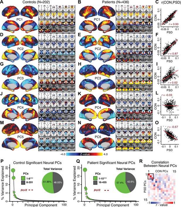
Principal component analysis (PCA) of neural features in control and patient subjects.

(A) Results of PCA performed on neural features (718 whole-brain parcel GBC) across all control subjects (N = 202). (B) Results of PCA performed on neural features (718 whole-brain parcel GBC) across all patient subjects (N = 436). (C) Note that the first neural PC in control subjects (panel A) and in patient subjects (panel B) are highly similar (r = 0.90 across parcels). This may reflect a component of neural variance common across all humans. (**D–I**) The second and third PCs are also similar between control and patient subjects. (**J–L**) The fourth PC is markedly dissimilar between control and patient subjects, suggesting that this component may reflect neural variance which deviates in individuals with psychiatric symptoms. (**M–O**) The fifth PC is also highly dissimilar between controls and patients, also possibly reflecting diagnosis-relevant differences in neural variance. (P) Screeplot showing the total proportion of variance explained by the first 100 PCs from the PCA performed across all 718 neural features in 202 control subjects. The size of each point is proportional to the variance explained by that PC. The first 8 PCs (green) were determined to be significant using a permutation test. Inset shows the proportion of variance both accounted and not accounted for by the eight significant PCs. Together, these 8 PCs capture 51.95% of the total variance in neural GBC in the sample. (Q) Screeplot showing the total proportion of variance explained by the first 100 PCs from the PCA performed across all 718 neural features in 436 patient subjects. The size of each point is proportional to the variance explained by that PC. The first 15 PCs (green) were determined to be significant using a permutation test. Inset shows the proportion of variance both accounted and not accounted for by the 15 significant PCs. Together, these five PCs capture 57.4% of the total variance in neural GBC in the sample. (R) Correlations between the first 15 neural PCs in controls (CON) and patients (PSD). The first three PCs are common across both control and patient subjects, possibly reflecting common components of human neural variance. After this, the PCs diverge, possibly reflecting differences in neural variance of healthy individuals and those with psychiatric symptoms.

Appendix 1—figure 20

Download asset Open asset

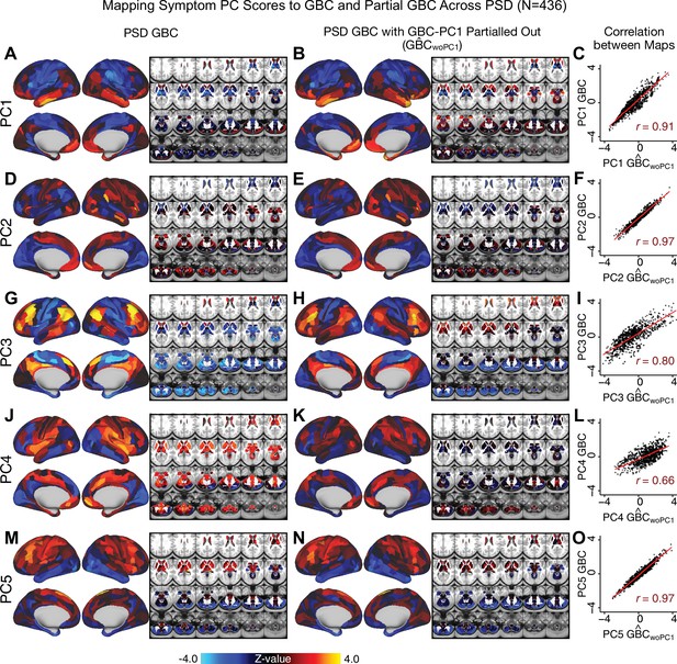
Comparison between the PSD $β_{P C} G B C$ maps computed using GBC and GBC with the first neural PC parsed out.

If a substantial proportion of neural variance is not be clinically relevant then removing the shared neural variance between PSD and CON should not drastically affect the reported symptom-neural univariate mapping solution, because this common variance will not map to clinical features. We therefore performed a PCA on CON and PSD GBC to compute the shared neural variance (see ***Materials and methods***), and then parsed out the first GBC-PC from the PSD GBC data ( ${\hat{G B C}}_{w o P C 1}$ ). We then reran the univariate regression as described in Figure 3, using the same five symptom PC scores across 436 PSD. (A) The $β_{P C 1} G B C$ map, also shown in Appendix 1—figure 10. (B) The first GBC-PC accounted for about 15.8% of the total GBC variance across CON and PSD. Removing GBC-PC1 from PSD data attenuated the $β_{P C 1} G B C$ statistics slightly (not unexpected as the variance was by definition reduced) but otherwise did not strongly affect the univariate mapping solution. (C) Correlation across 718 parcels between the two $β_{P C 1} G B C$ map shown in A and B. (**D–O**) The same results are shown for $β_{P C 2} G B C$ to $β_{P C 5} G B C$ maps.

Appendix 1—figure 21

Download asset Open asset

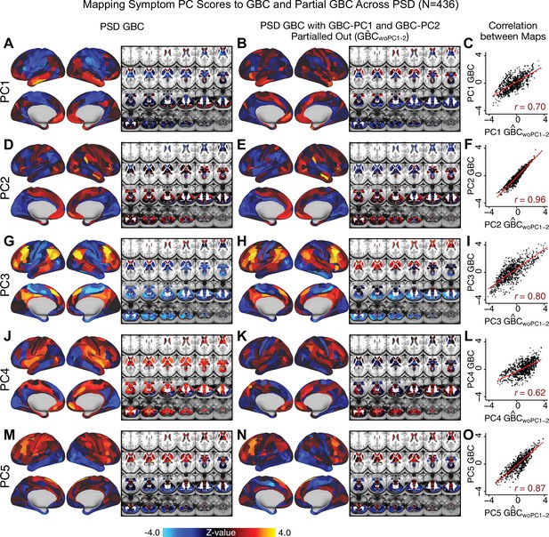
Comparison between the PSD $β_{P C} G B C$ maps computed using GBC and GBC with the first two neural PCs parsed out.

We performed a PCA on CON and PSD GBC and then parsed out the first three GBC-PC from the PSD GBC data ( ${\hat{G B C}}_{w o P C 1 - 2}$ , see **Materials and methods**). We then reran the univariate regression as described in Figure 3, using the same five symptom PC scores across 436 PSD. (A) The $β_{P C 1} G B C$ map, also shown in Appendix 1—figure 10. (B) The second GBC-PC accounted for about 9.5% of the total GBC variance across CON and PSD. (C) Correlation across 718 parcels between the two $β_{P C 1} G B C$ map shown in A and B. (**D–O**) The same results are shown for $β_{P C 2} G B C$ to $β_{P C 5} G B C$ maps.

Appendix 1—figure 22

Download asset Open asset

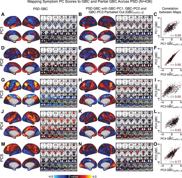
Comparison between the PSD $β_{P C} G B C$ maps computed using GBC and GBC with the first three neural PCs parsed out.

We performed a PCA on CON and PSD GBC and then parsed out the first three GBC-PC from the PSD GBC data ( ${\hat{G B C}}_{w o P C 1 - 3}$ , see **Materials and methods**). We then reran the univariate regression as described in Figure 3, using the same five symptom PC scores across 436 PSD. (A) The $β_{P C 1} G B C$ map, also shown in Appendix 1—figure 10. (B) The second GBC-PC accounted for about 9.5% of the total GBC variance across CON and PSD. (C) Correlation across 718 parcels between the two $β_{P C 1} G B C$ map shown in A and B. (**D–O**) The same results are shown for $β_{P C 2} G B C$ to $β_{P C 5} G B C$ maps.

Appendix 1—figure 23

Download asset Open asset

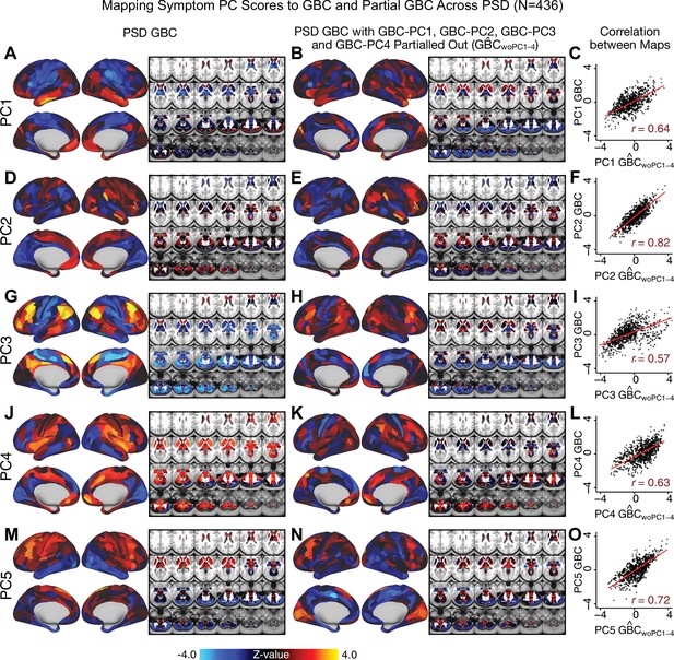
Comparison between the PSD $β_{P C} G B C$ maps computed using GBC and GBC with the first four neural PCs parsed out.

We performed a PCA on CON and PSD GBC and then parsed out the first four GBC-PC from the PSD GBC data ( ${\hat{G B C}}_{w o P C 1 - 4}$ , see ***Materials and methods***). We then reran the univariate regression as described in Figure 3, using the same five symptom PC scores across 436 PSD. (A) The $β_{P C 1} G B C$ map, also shown in Appendix 1—figure 10. (B) The second GBC-PC accounted for about 9.5% of the total GBC variance across CON and PSD. (C) Correlation across 718 parcels between the two $β_{P C 1} G B C$ map shown in A and B. (**D–O**) The same results are shown for $β_{P C 2} G B C$ to $β_{P C 5} G B C$ maps.

Appendix 1—figure 24

Download asset Open asset

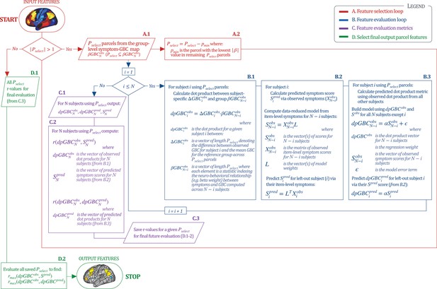
Workflow for optimizing the neural feature selection for a predictive symptom-neural subject specific model.

We optimized the selection of a subset of neural parcels from the group $β G B C_{N}^{o b s}$ map (where $N$ is the total number of subjects) that could be predicted via a single symptom score across subjects (e.g. for the *PC3* beta map and *PC3* symptom scores). (START) We start with $P_{s e l e c t}$ set as the full parcellated map, $P_{s e l e c t} = β G B C_{N}^{o b s}$ . Hence initially there are 718 elements in the vector $P_{s e l e c t}$ , each representing the value of a parcel ( $| P_{s e l e c t} | = 718$ ). Next, since $| P_{s e l e c t} | > 1$ , the selection process enters the A. Feature Selection Loop (in red). Selects subset of parcels $P_{s e l e c t}$ (A.1) for which the predictive model will be evaluated. This loop iteratively removes parcels from the $P_{s e l e c t}$ vector (A.2) and each time passes the updated $P_{s e l e c t}$ as input in the Feature Evaluation Loop (in blue). B. Feature Evaluation Loop (shown in blue). Using a multi-step algorithm, this loop produces the set of metrics to be evaluated at the final output using a leave-one-subject out approach. B.1: For each subject $i$ , this first step is to compute the ‘observed’ dot product metric $d p G B C_{i}^{o b s}$ for that subject. This is the dot product between $Δ G B C_{i}^{o b s}$ and $β G B C_{N - i}^{o b s}$ using the $P_{s e l e c t}$ features. $Δ G B C_{i}^{o b s}$ is the vector of the parcel-wise difference between subject $i$ ’s GBC map and the group mean GBC map; $β G B C_{N - i}^{o b s}$ denotes group-level relationship between symptom variation and GBC excluding subject $i$ . This group $β G B C_{N - i}^{o b s}$ is used as a reference for the dot-product. B.2: Next for subject $i$ we compute their predicted symptom score $S_{i}^{p r e d}$ . First, a symptom-prediction model is built using $X_{N - i}^{o b s}$ (all item-level symptom measures excluding subject $i$ ). This yields the ‘observed’ model scores and coefficients excluding subject $i$ ( $S_{N - i}^{o b s}$ ). The symptoms for excluded subject $i$ are then used to obtain the predicted symptom score $S_{i}^{p r e d}$ , as done in Figure 6A. B.3: Lastly, for excluded subject $i$ the loop computes the ”predicted’ dot product metric $d p G B C_{i}^{p r e d}$ to compare it to the ”observed’ value for model evaluation. Here, a regression model is computed relating $d p G B C_{N - i}^{o b s}$ to $S_{N - i}^{o b s}$ , excluding subject $i$ . This yields regression coefficients α, which are then used to predict the $d p G B C_{i}^{p r e d}$ for the excluded subject $i$ using their predicted symptom scores $S_{i}^{p r e d}$ . Once $i > N$ (i.e. $d p G B C_{i}^{p r e d}$ and $S_{i}^{p r e d}$ have been computed for all subjects), the algorithm moves to step ”C’. C. Feature Evaluation Metrics (shown in purple). C.1: This step captures feature evaluation metrics across N subjects for the model that was computed using the selected features ( $P_{s e l e c t}$ ). Specifically, three vectors (outputs from ‘B’) are computed: $d p G B C_{N}^{o b s}$ (the vector of observed $d p G B C$ values for all $N$ subjects); $d p G B C_{N}^{p r e d}$ (the vector of predicted $d p G B C$ values for all $N$ subjects); and $S_{N}^{p r e d}$ (the vector of predicted model symptom scores for all $N$ subjects). C.2: Generates two feature evaluation metrics across the entire sample ( $r (d p G B C_{N}^{o b s}, S_{N}^{p r e d})$ and $r (d p G B C_{N}^{o b s}, d p G B C_{N}^{p r e d})$ ). C.3: The feature evaluation metrics for the selected $P_{s e l e c t}$ are generated, such that they can be evaluated across all $P_{s e l e c t}$ iterations (red loop). D. Final Feature Selection (in green). This step evaluates the metrics computed for all $P_{s e l e c t}$ iterations, starting from from $| P_{s e l e c t} | = 718$ to $| P_{s e l e c t} | = 1$ . D.1: The input is the vector of $r (d p G B C_{N}^{o b s}, S_{N}^{p r e d})$ and the vector of $r (d p G B C_{N}^{o b s}, S_{N}^{p r e d})$ for all 718 models. D.2: The most predictive feature subset is obtained by finding the model for which $r (d p G B C_{N}^{o b s}, S_{N}^{p r e d})$ and $r (d p G B C_{N}^{o b s}, d p G B C_{N}^{p r e d})$ were maximized, which leads to the final output features (STOP). *Note*: that the algorithm imposed a threshold of $| P_{s e l e c t} | > 30$ to ensure that the correlation metrics were not unstable based on a small feature set.

Appendix 1—figure 25

Download asset Open asset

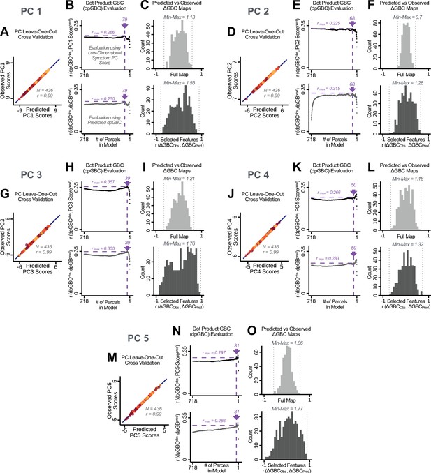
Optimizing neural feature selection to inform statistically reliable single-subject prediction via low-dimensional symptom scores only.

(A) Individual PC-derived symptom scores for *PC1* can be robustly predicted, as shown by leave-one-out cross-validation for the symptom PCA analyses. Here for the leave-one-out cross-validation, a PCA was computed in all except one subject (N = 435) and the PCA loadings were then used to compute the predicted PC scores for the left-out subject. This was repeated such that predicted scores were calculated for every subject, using loadings from a PCA computed in the other 435 subjects. Observed scores were obtained from a PCA computed using the full sample of subjects (N = 436). Top panel: Scatterplot at left shows the correlation between each subject's predicted *PC1* score from leave-one-out PCA model and their observed *PC1* score from the full-sample PCA model, r = 0.99. Red line shows perfect prediction, r = 1. (B) Top panel indicates that PC symptom scores can yield robust neural feature selection. ΔGBC denotes an individual subject GBC demeaned parcel-wise relative to the group mean GBC. The process is described in detail in the **Materials and methods** and in Appendix 1—figure 26. The correlation between *PC1* behavioral score and [ΔGBC · *PC1* beta] across all 436 subjects was maximal for $P = 79$ , at r = 0.27 (purple arrow). Bottom panel: For each value of p, the regression was performed in 435 subjects and was then used to predict the [ΔGBC · *PC1* beta] of the selected parcels in the left-out subject. The mean correlation between the predicted [ΔGBC·*PC1* beta] and the actual observed [ΔGBC · *PC1* beta] across all 436 subjects was highest for $P = 79$ , with r = 0.19 across all subjects, highly consistent with the across-subject analysis in the top panel. (C) Comparing the correlation between $Δ G B C^{o b s}, Δ G B C^{p r e d}$ , for the full map ( $P = 718$ ) versus the selected map ( $P = 79$ ) shows that the predictability of $Δ G B C$ is improved by using the selected parcels in the selected maps. (**D–O**) Similar results for PCs 2–5. Note that for *PC4* and *PC5* a local maximum ( $P = 50$ and $P = 31$ respectively) was selected after imposing a threshold of $P > 30$ to ensure that the correlation metrics used for evaluation were not made unstable from a small number of parcels in computing the $d p G B C$ .

Appendix 1—figure 26

Download asset Open asset

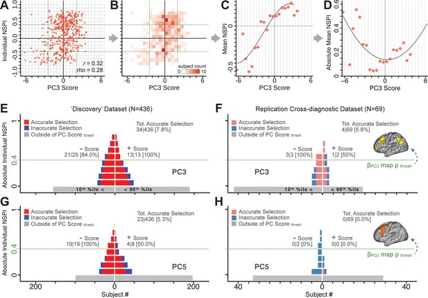
Evaluating patient-specific similarity to derived symptom-neural targets via data-reduced symptom scores.

(A) Scatterplot of *PC3* symptom score (X-axis) versus *PC3* neural similarity prediction index (NSPI, Y-axis) for all 436 PSD subjects. The NSPI is defined as the Spearman’s correlation between $Δ G B C^{o b s}$ and the $β_{P C 3} G B C^{o b s}$ map of the maximally-predictable ‘selected’ $P = 39$ parcels. Alternative metrics are shown in Appendix 1—figure 28. (B) Bins across axes express subject counts within each cell as a heatmap, indicating a high similarity between symptom PC score and *PC3* NSPI for a number of patients. (C) Mean NSPI is computed for a given bin along the the X-axis to visualize patient clustering. Note the sigmoidal shape of the distribution reflecting greater neural similarity at more extreme values of the *PC3* score. (D) The absolute value of the mean NSPI reflects the magnitude irrespective of neural similarity direction. This highlights a quadratic effect, showing that patients with higher *PC3* symptom scores (either positive/negative) exhibited higher neural correspondence of their maps with the target neural reference map. (E) Using the NSPI and PC scores we demonstrate one possible brain-behavioral patient selection strategy. We first imposed a PC score symptom threshold to select patients at the extreme tails (i.e. outside of the $10 t h - 90 t h % t i l e$ behavioral range [>+2.17 or <−2.41]). Note that this patient selection strategy excludes patients (shown in gray) below the PC symptom score threshold. This yielded n = 38 patients. Next, for each patient we predicted the sign of their individual NSPI based on their individual PC3 score, which served as the basis for the neural selection. Next, at each NSPI threshold we evaluated the proportion of patients correctly selected until there were no inaccurately selected patients in at least one PC3 direction (green line or higher). The number of accurately (A) vs. inaccurately (I) selected patients within each bin is shown in red and blue respectively. Note that as the neural ρ threshold increases the A/I ratio increases. (F) The neural and behavioral thresholds defined in the ‘discovery’ sample were applied to an independent ‘replication’ dataset (N = 69, see **Materials and methods**), yielding a similar final proportion of accurately selected patients. (G) The same brain-behavioral patient selection strategy was repeated for *PC5* in the discovery sample (thresholds of $10^{t h} % t i l e$ = −1.89 and $90^{t h} % t i l e$ = +1.47; NSPI threshold of ρ = 0.4 optimized for PC5). Results yielded similar A/I ratios as found for PC3. (H) The neural and behavioral thresholds for PC5 defined in the discovery sample were applied to the replication sample. Here the results failed to generalize due true clinical differences between the discovery and replication samples.

Appendix 1—figure 27

Download asset Open asset

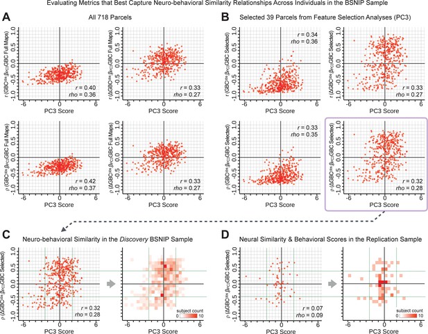
Metrics quantifying the relationship between individual-level neural effects relative to the group mean and individual-level PC-derived symptom scores.

The relationship between various symptom-neural similarity metrics and the behavioral *PC3* symptom scores across N = 436 PSD patients are shown. The goal was to evaluate metrics that maximize the spread of the Y-axis, while maintaining a centered distribution of scores around zero to yield an interpretable symptom-neural variation pattern across subjects. Specifically, along the Y-axis we examined either the Pearson’s correlation (top panels in A and B) or Spearman’s ρ (bottom panels in A and B) between two neural maps at the individual patient level: (i) the group-level $β_{P C 3} G B C$ map and (ii) an individual subjects’ raw GBC map which can be expressed as either a raw map (left panels in A and B) or as $Δ G B C^{o b s}$ relative to the group mean map (right panels in A and B). (A) These four panels show group-level symptom-neural relationships for sample using the entire 718-parcel neural map. As noted, the neural similarity metrics on each Y-axis show the relationship between individual-patient neural GBC (or $Δ G B C^{o b s}$ ) and the group-level $β_{P C 3} G B C$ map across 718 parcels. Note that the r and *rho* values reported in the corner of each plot reflect the *group-level* relationship between the neural similarity metric and the individual-level PC3 symptom score computed across across 436 patients. (B) These four parcels show group-level symptom-neural relationships using only the selected 39 *PC3* parcels derived from the feature selection workflow (Appendix 1—figure 25). The metric used in the main text is the ρ within selected parcels (shown with a light purple envelope) because the spread along Y-axis was maximized and the values centered around zero for both the x and the Y-axis. Furthermore, the ρ metric is desirable given violations of normality that the $r$ metric assumes. (C) The neural-behavioral similarity plot for the Discovery BSNIP sample was binned by $ρ = 0.1$ & $P C 3_{s c o r e} = 0.5$ to provide a visual intuition for patient segmentation across both the neural and symptom indices. For patients with highly positive or negative scores, the neuro-behavioral relationship was robust. Conversely, patients with a low absolute *PC3* score showed a weak relationship with symptom-relevant neural features. (D) The neural-behavioral similarity plot for the independent replication sample (see **Materials and methods** for sample details) was binned by $ρ = 0.1$ & $P C 3_{s c o r e} = 0.5$ , using the same neural similarity index (ρ[ $Δ G B C^{o b s}$ , $β_{P C 3} G B C^{o b s}$ ] within selected 39 parcels) and projected *PC3* symptom scores. Although the grid is far more sparse (total N = 69 for this sample), a similar pattern between PC3 symptom score and neural similarity index emerges.

Appendix 1—figure 28

Download asset Open asset

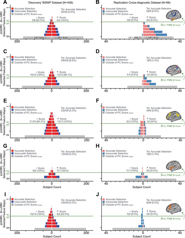
Evaluating patient-specific similarity to derived symptom-neural targets via data-reduced symptom scores for all *PCs*.

As noted in the main text for *PC3*, here we plot the PC symptom score (X-axis) versus the neural similarity prediction index (NSPI, Appendix 1—figure 26) for all 436 PSD patients. The NSPI is defined as the Spearman’s correlation between $Δ G B C^{o b s}$ and the $β_{P C 3} G B C^{o b s}$ map of the maximally-predictable ‘selected’ $P$ parcels (Y-axis for each plot). Alternative metrics were evaluated in Appendix 1—figure 27. (A) A parameter sweep was performed for 0<|rho|<1 in bins of 0.1, for all subjects with *PC1* score<−3.97 ‘negative behavioral threshold’ set at the 10th percentile (P_90-Disc) of the distribution and for all patients with *PC1* score >+3.60 (‘positive behavioral threshold’ set at the 90th percentile (P_90-Disc) of the distribution). The number of patients accurately selected within each bin is shown in red; the number of inaccurately selected patients is shown in blue. Note that this selection process excludes a number of patients (shown in gray) who do not meet the PC threshold cutoff. Note that as the neural ρ threshold increases the proportion of accurate to inaccurate selections increases and the number of inaccurately selected subjects decreases. For illustrative purposes, a neural threshold of ρ = 0.5 is applied at the point where no inaccurate selections occur for the positive behavioral threshold. (B) The neural and symptom score thresholds defined in discovery patients were applied on an independent external ‘replication’ dataset (N = 69, see **Materials and methods**). For the symptom score (p_90-Disc = −3.97 and p_90-Disc = +3.60 ) and neural (ρ = 0.5) thresholds as those defined in the discovery sample, no patients are selected for *PC1*. (**C–D**) Similar data to A–B for *PC2*, using PC score thresholds of p_90-Disc = −2.43 and p_90-Disc = +2.32 and a PC map threshold of ρ = 0.3 on a subset of $P = 68$ optimized parcels. (**E–F**) Similar data to A–B for *PC3* using PC score thresholds of p_90-Disc = −2.41 and p_90-Disc = +2.17 and a PC map threshold of ρ = 0.4 on a patients of $P = 39$ optimized parcels. (**G–H**) Similar data to A–B for *PC4*, using PC score thresholds of p_90-Disc = −1.69 and p_90-Disc = +1.72 and a PC map threshold of ρ = 0.2 on a subset of $P = 50$ optimized parcels. (**I–J**) Similar data to A–B for *PC5*, using PC score thresholds of p_90-Disc = −1.89 and p_90-Disc = +1.47 and a PC map threshold of ρ = 0.4 on a subset of $P = 31$ optimized parcels.

Appendix 1—figure 29

Download asset Open asset

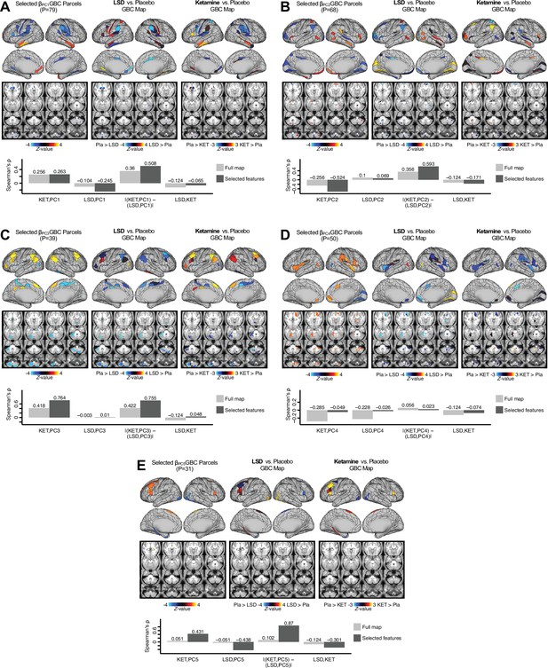
Examining most predictive parcels for all PC-driven symptom-neural effects and their relationship with pharmacological neuroimaging maps.

(A) (Left) The selected group-level $β_{P C 1} G B C$ map showing the 79 selected parcels derived from the feature selection workflow (Appendix 1—figure 25). (Middle) The same parcels are highlighted from the group-level $Δ G B C$ LSD map reflecting the pharmacological effect relative to placebo. (Right) the group-level ketamine $Δ G B C$ map reflecting the pharmacological effect relative to placebo. (Bottom bar plot) Here we show four values: (i) Spearman’s ρ between the ketamine $Δ G B C$ and $β_{P C 1} G B C$ maps (KET,PC1); (ii) Spearman’s ρ between the LSD $Δ G B C$ and $β_{P C 1} G B C$ maps (LSD,PC1); i(ii) Absolute value of the difference for the (i) and (ii), i.e. differential similarity; |(KET,PC1) - (LSD,PC1)|; (iv) Spearman’s ρ between the ketamine $Δ G B C$ response and LSD ketamine $Δ G B C$ response maps (KET,LSD). These relationships are quantified within both the selected 79 features (dark gray bars) and the full P=718 neural map (light gray bars). (**B–E**) These analyses are repeated and shown for *PCs 2–5*. Note that a strong differential similarity for a pair of pharmacological maps may indicate a strategy for patient treatment selection along a particular brain-behavioral axis. Specifically, in this framework patients loading on *PC3* behaviorally (or neurally) would be indicated as highly similar to neural variation induced by ketamine but not LSD. Such metrics may be clinically useful for selecting one pharmacological target over another in the process making individual patient segmentation decisions.

Appendix 1—figure 30

Download asset Open asset

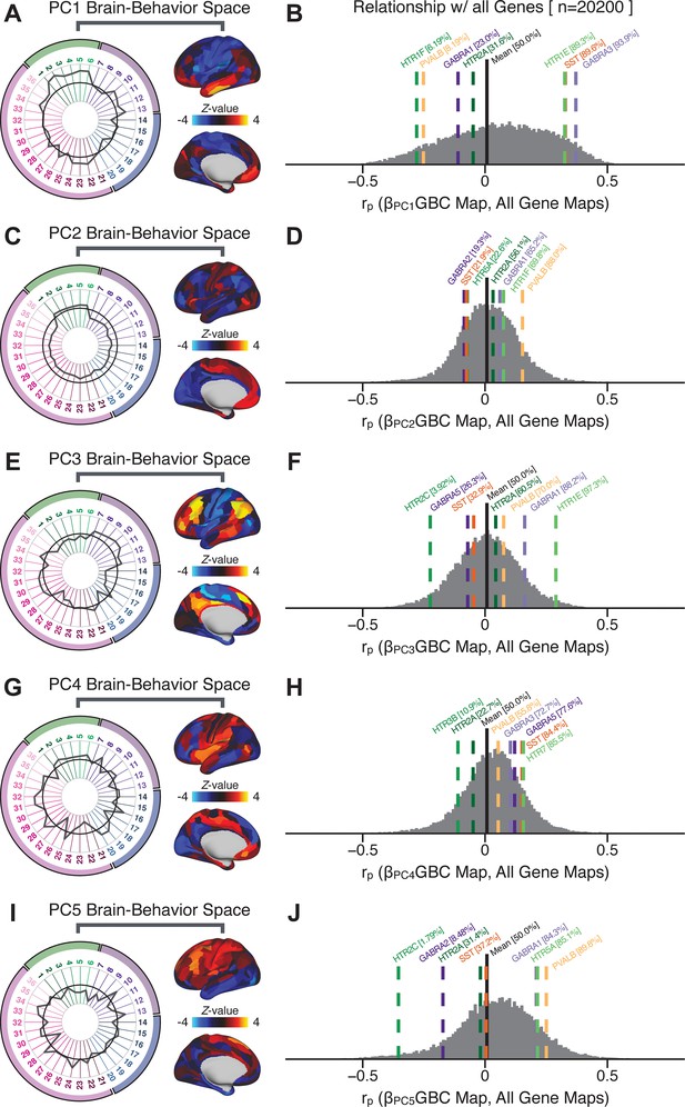
Quantifying the relationship between PC-derived symptom-neural effects and expression maps for genes implicated in psychosis spectrum disorder (PSD) neurobiology.

(A) The symptom loading profile (radarplot) and neural loading map derived in the main analyses are shown for the *PC1* BBS. (B) The distribution shows the Pearson’s correlation coefficients between the *PC1* symptom-neural map and all 20,200 gene expression maps derived from the Allen Human Brain Atlas (AHBA, see **Materials and methods** and for details on gene expression analyses see [Burt et al., 2018]). In this analysis we focused on a select number of PSD-relevant genes, as highlighted in the main text for PC3 specifically Figure 8. Seven genes of interest are shown. Specifically, these include two interneuron marker genes, somatostatin (SST) and parvalbumin (PVALB); two GABA_A receptor subunit genes: GABRA1 and GABRA3; and three serotonin receptor subunit genes: HTR1E, HTR1F, and HTR2A. The percentile for each highlighted gene relative to the entire distribution of 20,200 genes is reported in square brackets. Note that the gene expression maps of HTR1F and PVALB are at the negative tail of the entire distribution, that is, anti-correlated with *PC1* symptom-neural map. Conversely, GABRA3, SST, and HTR1E are on the far positive end, reflecting a highly similar spatial pattern of the gene expression maps with the *PC1* symptom-neural map. (**C–J**) PC symptom-neural map profiles and distributions of gene expression map similarities are also shown for PCs 2–5. Note that some of these exemplar genes show a strong spatial similarity (or anti-similarity) with the PC-derived neural maps relative to the entire distribution of all gene-PC map pairs.

Tables

Appendix 1—table 1

Glossary of the key terms and abbreviations used in the study.

Abbreviation/Term	Definition
General and Behavioral Terms
$P S D$	Psychosis spectrum disorder; or patients diagnosed with a PSD.
$B P P$	Bipolar disorder with psychosis; or patients diagnosed with BPP.
$S A D P$	Schizoaffective disorder with psychosis; or patients diagnosed with SADP.
$S Z P$	Schizophrenia with psychosis; or patients diagnosed with SZP.
$C O N$	Control subjects.
$B A C S$	Brief Assessment of Cognition in Schizophrenia.
$P A N S S$	Positive and Negative Syndrome Scale.
$S y m p t o m m e a s u r e s$	The 36 behavioral items from the BACS and PANSS.
$P C A, P C$	Principal component analysis, and principal component.
$I C A, I C$	Independent component analysis, and independent component.
Neural Terms
$F C$	Functional connectivity (Fisher's r-to-Z transformed Pearson correlation values).
$G B C$	Global brain connectivity; computed for each brain location as the the mean FC across the whole brain.
$β_{P C} G B C$	The beta coefficient map from a mass univariate regression of PC scores on to GBC across subjects.
$β_{P C} G B C^{o b s}$	The beta coefficient map from a mass univariate regression of observed (measured) symptom PC scores on to observed (measured) GBC across subjects.
$β_{P C} G B C^{p r e d}$	The beta coefficient map from a mass univariate regression of predicted symptom PC scores on to observed (measured) GBC across subjects.
$G B C - P C A$	A PCA performed on the neural GBC data across all N = 638 PSD and CON subjects.
${\hat{G B C}}_{w o P C 1}$	The GBC matrix reconstructed without the first PC of the GBC-PCA.
${\hat{G B C}}_{w o P C 1 - 2}$	The GBC matrix reconstructed without the first two PCs of the GBC-PCA.
${\hat{G B C}}_{w o P C 1 - 3}$	The GBC matrix reconstructed without the first three PCs of the GBC-PCA.
${\hat{G B C}}_{w o P C 1 - 4}$	The GBC matrix reconstructed without the first four PCs of the GBC-PCA.
Multivariate Analyses Terms
$C C A$	Canonical correlation analysis.
$C V$	Canonical variate from a CCA solution.
$180 v s . 36 C C A$	The CCA computed between 180 neural features and 36 symptom measures.
$5180 v s . 5 C C A$	The CCA computed between 180 neural features and five symptom PCs.
$N, B$	The input neural and behavioral data matrices in a CCA, respectively.
$\hat{N}, \hat{B}$	The predicted neural and behavioral data matrices in the CCA cross-validation, respectively.
$Θ, Ψ$	The neural and behavioral transformation matrices in a CCA, respectively.
$U, V$	The transfomed neural and behavioral data matrices in a CCA, respectively.
Single-Subject Prediction Analyses Terms
$Δ G B C$	The difference between an individual's measured GBC map and the mean GBC map computed for the whole group; reflects individual differences in GBC, which may otherwise be conflated by the group mean.
$β_{P C} G B C_{N - 1}^{o b s}$	The beta coefficient map computed across $N - 1$ subjects, using observed symptom PC and GBC data.
$S^{o b s}$	The vector of observed symptom scores for a single PC (i.e. from a PCA computed using symptom measures), with length N-1 (as subject i is left out).
$S^{p r e d}$	The predicted symptom PC for subject $i$ , using the loadings from a leave-one-out PCA computed on N-i subjects.
$d p G B C$	Dot product between a subject's ΔGBC map and a β_PCGBC map.
$d p G B C_{i}^{o b s}$	Dot product between a subject $i$ 's ΔGBC map and the $β_{P C} G B C_{N - 1}^{o b s}$ map computed without that subject.
$d p G B C_{i}^{p r e d}$	The predicted dpGBC for a subject $i$ , predicted from a regression model using the dpGBCobs from all other subjects and the predicted Spred for subject $i$ .
$P_{s e l e c t}$	The number of parcels in the subset of the brain map used in a particular analysis. $P_{s e l e c t} = 718$ for the full whole-brain map.
$B B S$	Brain-Behavior Space; the symptom and neural mapping for a particular dimension.

Appendix 1—table 2

Clinical and demographic details for the BSNIP sample.

Clinical and demographic measures are shown at the group level for the BSNIP sample used for initial ‘discovery’ analyses. Means and standard deviations were computed for each of the diagnostic groups. Abbreviations: CON, controls; PSD, psychosis spectrum disorder patients; BPP, bipolar disorder with psychosis; SADP, schizoaffective disorder with psychosis; SZP, schizophrenia; CPZ, chlorpromazine; PANSS, Positive and Negative Syndrome Scale for Schizophrenia, BACS, Brief Assessment of Cognition in Schizophrenia.

Characteristic	CON (N=202)		PSD (N=436)		BPP (N=150)		SADP (N=119)		SZP (N=167)
	Mean	SD	Mean	SD	Mean	SD	Mean	SD	Mean	SD
Age (years)	37.18	12.18	35.33	12.31	36.29	12.94	35.86	11.87	34.16	11.99
Sex (% male)	42.08	-	48.62	-	31.33	-	44.54	-	67.07	-
Parental Education (years)	13.35	3.42	13.67	3.43	14.16	3.44	13.05	3.95	13.62	2.93
Participant’s Education	14.76	2.27	13.47	2.34	14.22	2.31	13.25	2.22	12.93	2.28
Handedness (% right)	85.64	-	85.78	-	83.33	-	88.24	-	86.23	-
Signal-to-Noise (SNR)	231.03	82.70	218.34	93.44	229.78	100.09	230.93	93.83	198.10	83.13
% Frames Flagged	2.81	3.99	6.17	9.09	6.41	9.67	5.32	9.32	6.57	8.35
Medication (CPZ equivalents)	-	-	443.20	402.92	318.61	321.06	514.43	462.70	490.64	395.76
PANSS Positive Symptoms	7.03	0.30	15.66	5.35	12.87	4.35	18.19	5.20	16.37	5.15
PANSS Negative Symptoms	7.01	0.16	14.59	5.10	12.01	3.66	15.55	4.52	16.22	5.68
PANSS General Psychopathology	16.04 0.36	31.45	8.67	28.72	8.20	34.57	8.70	31.67	8.30
PANSS Total Psychopathology	30.08	0.61	61.67	16.32	53.59	13.69	68.22	15.72	64.26	16.04
BACS Cognitive Score (Z)	0.02	1.10	−1.22	1.20	−0.83	1.19	−1.30	1.10	−1.52	1.19

Appendix 1—table 3

Scan acquisition parameters for the BSNIP dataset across sites.

Scan acquisition details are shown for the 6 BSNIP acquisition sites. Adapted from Meda et al., 2015.

BOLD	TR (ms)	TE (ms)	FA (deg.)	Slices (N)	Slice order	Matrix (mm)	Voxel (mm)	Vendor
Baltimore	2210	30	70	36	I-A	64 × 64	3.4 × 3.4 × 3	Siemens Trio
Hartford	1500	27	70	29	S-A	64 × 64	3.4 × 3.4 × 5	Siemens Allegra
Detroit	1570/1720	22	60	29	S-A	64 × 64	3.4 × 3.4 × 4	Siemens Trio
Dallas	1500	27	60	29	S-A	64 × 64	3.4 × 3.4 × 4	Philips
Chicago	1775	27	60	29	S-A	64 × 64	3.4 × 3.4 × 4	GE Signa HDX
Boston	3000	27	60	30	S-A	64 × 64	3.4 × 3.4 × 5	GE Signa HDX
T1w	TR (ms)	TE (ms)	FA (deg.)	Slices (N)	Slice order	Matrix (mm)	Voxel (mm)	Vendor
Baltimore	2300	2.91	9	160	—	256 × 240	1 × 1 × 1.2	Siemens Trio
Hartford	2300	2.91	9	160	—	256 × 240	1 × 1 × 1.2	Siemens Allegra
Detroit	2300	2.94	9	160	—	256 × 240	1 × 1 × 1.2	Siemens Trio
Dallas	6.6	2.8	8	170	—	256 × 256	1 × 1 × 1.2	Philips
Chicago	6.98	2.84	8	166	—	256 × 256	1 × 1 × 1.2	GE Signa HDX
Boston	6.98	2.84	8	166	—	256 × 256	1 × 1 × 1.2	GE Signa HDX

Appendix 1—table 4

Clinical and demographic details for the independent replication cross-diagnostic sample.

Clinical and demographic measures are shown at the group level for the independent clinical sample used for replication analyses presented in main text (Figure 7). Means and standard deviations were computed for each of the diagnostic groups. Abbreviations: CON, controls; PTT, all patients; OCD, obsessive-compulsive disorder; SZP, schizophrenia; PANSS, Positive and Negative Syndrome Scale for Schizophrenia, BACS, Brief Assessment of Cognition in Schizophrenia.

Characteristic	CON (N=34)		PTT (N=69)		OCD (N=39)		SZP (N=30)
	Mean	SD	Mean	SD	Mean	SD	Mean	SD
Age (years)	29.91	8.11	33.7	12.89	32.23	12.32	35.63	13.63
Sex (% male)	61.7	-	59.4	-	46.1	-	76.7	-
Parental Education (years)	15.05	3.31	13.98	3.45	14.02	3.78	13.93	3.01
Participant’s Education	16.37	2.34	14.16	2.12	15.22	1.95	12.79	2.34
Handedness (% right)	93.9	-	91.3	-	84.6	-	100.0	-
Signal-to-noise (SNR)	53.45	5.59	51.86	5.63	52.29	5.28	51.33	6.08
% Frames Flagged	0.21	0.53	7.27	15.53	5.11	13.81	10.07	17.37
PANSS Positive Symptoms	7.58	1.06	11.40	4.23	8.97	2.74	14.56	6.16
PANSS Negative Symptoms	7.75	1.57	11.06	3.59	8.80	2.21 14.00	5.39
PANSS General Psychopathology	32.62	2.62	48.80	10.96	42.71	9.07 56.72	13.42
PANSS Total Psychopathology	47.95	5.25	71.26	18.78	60.48	14.02 85.28	24.97
BACS Cognitive Score (Z)	0.00	1.00	−0.67	1.45	−0.07	1.03	−1.45	1.55

Appendix 1—table 5

Summary of the key questions, results, and supporting data in this study.

Question	Results	Corresponding Figures
Can data-reduction methods (e.g. principal component analysis, PCA) reliably map symptom axes across PSD that include both canonical symptoms and cognitive deficits?	The PCA on 36 behavioral measures and 436 PSD patients produced five significant components (PCs) spanning key symptom domains and oblique to conventional symptom factors and diagnostic categories.	Figure 1
		Appendix 1—figure 2–3
Are the derived dimensionality-reduced symptom axes in PSD stable and replicable?	The behavioral PCA solution was stable across split-half replication, leave-site-out, and k-fold cross-validations, and not driven by medication effects.	Figure 2
		Appendix 1—figure 4, 5, 6, 7
Do dimensionality-reduced symptom axes yield stronger statistical neural maps across PSD, relative to conventional scales & diagnoses?	PC symptom scores yielded a much stronger statistical effect with neural features (as measured by global brain connectivity, GBC) across patients than did conventional symptom scores.	Figure 3
		Appendix 1—figures 7, 8, 9, 10
Are the PC brain-behavior maps stable and replicable?	PC brain-behavior maps are stable and reproducible across split-half, leave-site-out and k-fold cross-validations.	Figure 4
Are the PC brain-behavior maps stable and replicable?		Appendix 1—figure 11–12
Can a multivariate approach (e.g. canonical correlation analysis, CCA) be used to derive a stable neuro-behavioral mapping?	CCA produced a stable within-sample solution, but performed poorly on out-of-sample cross-validations.	Figure 5
		Appendix 1—figures 13, 14, 15, 16, 17, 18
8Is the computed symptom-to-neural mapping actionable for individual patient selection?	A majority of neural variance in PSD patients is not symptom-relevant. However, brain-behavioral maps can be optimized to select specific patients along PC axes. This method can also be applied to select patients from independent datasets.	Figures 6 and 7
		Appendix 1—figures 24, 25, 26, 27, 28
8Can we inform molecular mechanism and treatment decisions by relating patient-specific brain-behavioral maps to independently-acquired pharmacological neuroimaging maps?	Pharmacological neuroimaging maps targeting mechanisms of interest (e.g. ketamine and LSD) can be used as independent benchmarks against which patient-specific brain-behavioral maps can be evaluated.	Figure 7
		Appendix 1—figure 29
9Can we inform molecular mechanism and potential novel therapeutic targets by relating brain-behavior maps to gene expression maps?	Gene expression maps for genes implicated in PSD neuropathology (e.g. serotonin and GABA receptors, interneuron markers) can inform mechanism and potential novel targets relating to specific axes of neuro-behavioral variation.	Figure 8
		Appendix 1—figure 30

Additional files

Transparent reporting form: https://cdn.elifesciences.org/articles/66968/elife-66968-transrepform-v1.pdf
Download elife-66968-transrepform-v1.pdf

Download links

A two-part list of links to download the article, or parts of the article, in various formats.

Downloads (link to download the article as PDF)

Article PDF

Open citations (links to open the citations from this article in various online reference manager services)

Mendeley

Cite this article (links to download the citations from this article in formats compatible with various reference manager tools)

Jie Lisa Ji
Markus Helmer
Clara Fonteneau
Joshua B Burt
Zailyn Tamayo
Jure Demšar
Brendan D Adkinson
Aleksandar Savić
Katrin H Preller
Flora Moujaes
Franz X Vollenweider
William J Martin
Grega Repovš
John D Murray
Alan Anticevic

(2021)

Mapping brain-behavior space relationships along the psychosis spectrum

eLife 10:e66968.

https://doi.org/10.7554/eLife.66968

Share this article

Cite this article

Quantifying data-driven low-dimensional variation of cross-diagnostic psychosis spectrum disorder (PSD) symptoms and cognitive deficits.

Dimensionality reduction of PSD symptom measures is highly stable and reproducible.

Dimensionality-reduced symptom variation reveals robust neurobehavioral mapping.

Parcellated symptom-neural GBC maps reflecting psychosis configuration are statistically robust and reproducible.

Multivariate symptom-neural feature mapping using canonical correlation analysis (CCA).

Optimizing neural feature selection to inform single-subject prediction via a low-dimensional symptom solution.

Leveraging subject-specific brain-behavioral maps for molecular neuroimaging target selection.

Psychosis spectrum symptom-neural maps track neural gene expression patterns computed from the Allen Human Brain Atlas (AHBA).

Study workflow used study to quantify shared neural and behavioral variation in individuals diagnosed with PSD.

Alternative views of the behavioral PCA triplot.

Independent component analysis (ICA) as an alternative method of dimensionality-reduction of symptom data.

k-Fold cross-validation for symptom-driven principal component analysis (PCA).

Leave-site-out cross-validation for symptom-driven principal component analysis (PCA).

PCA solution is not driven by medication status or dosage.

Effects of age, socio-economic status, and sex on symptom PCA solution.

Similarity across a priori, categorical and PCA-derived brain-behavioral GBC maps.

Parcellated symptom-neural GBC maps across all PSD patients derived from PCA dimensionality reduction of symptom measures.

Parcellated symptom-neural GBC maps across all CON subjects derived from PCA dimensionality reduction of PSD symptom measures.

Individual patients exhibit complex projections into the PCA-derived brain-behavioral space (BBS) geometry (A) The PC3 group-level cortical map is shown here for comparison purposes.

Independent component analysis (ICA) as an alternative method of dimensionality-reduction for symptom-neural mapping.

Canonical correlation analysis (CCA) of behavioral and subcortical neural features.

Canonical correlation analysis (CCA) of behavioral and network-level neural features.

Canonical correlation analysis (CCA) results showing the amount of variance explained in the neural features via behavioral canonical variates.

Canonical correlation analysis (CCA) symptom and neural configurations.

K-Fold cross-validation of canonical correlation analysis (CCA).

Multivariate power analysis for CCA.

Principal component analysis (PCA) of neural features in control and patient subjects.

Comparison between the PSD βP⁢C⁢G⁢B⁢C maps computed using GBC and GBC with the first neural PC parsed out.

Comparison between the PSD βP⁢C⁢G⁢B⁢C maps computed using GBC and GBC with the first two neural PCs parsed out.

Comparison between the PSD βP⁢C⁢G⁢B⁢C maps computed using GBC and GBC with the first three neural PCs parsed out.

Comparison between the PSD βP⁢C⁢G⁢B⁢C maps computed using GBC and GBC with the first four neural PCs parsed out.

Workflow for optimizing the neural feature selection for a predictive symptom-neural subject specific model.

Optimizing neural feature selection to inform statistically reliable single-subject prediction via low-dimensional symptom scores only.

Evaluating patient-specific similarity to derived symptom-neural targets via data-reduced symptom scores.

Metrics quantifying the relationship between individual-level neural effects relative to the group mean and individual-level PC-derived symptom scores.

Evaluating patient-specific similarity to derived symptom-neural targets via data-reduced symptom scores for all PCs.

Examining most predictive parcels for all PC-driven symptom-neural effects and their relationship with pharmacological neuroimaging maps.

Quantifying the relationship between PC-derived symptom-neural effects and expression maps for genes implicated in psychosis spectrum disorder (PSD) neurobiology.

Glossary of the key terms and abbreviations used in the study.

Clinical and demographic details for the BSNIP sample.

Scan acquisition parameters for the BSNIP dataset across sites.

Clinical and demographic details for the independent replication cross-diagnostic sample.

Summary of the key questions, results, and supporting data in this study.

Transparent reporting form

Downloads (link to download the article as PDF)

Open citations (links to open the citations from this article in various online reference manager services)

Cite this article (links to download the citations from this article in formats compatible with various reference manager tools)

Comparison between the PSD $β_{P C} G B C$ maps computed using GBC and GBC with the first neural PC parsed out.

Comparison between the PSD $β_{P C} G B C$ maps computed using GBC and GBC with the first two neural PCs parsed out.

Comparison between the PSD $β_{P C} G B C$ maps computed using GBC and GBC with the first three neural PCs parsed out.

Comparison between the PSD $β_{P C} G B C$ maps computed using GBC and GBC with the first four neural PCs parsed out.