Motor cortex activity across movement speeds is predicted by network-level strategies for generating muscle activity
Figures
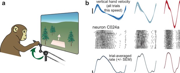
Illustration of behavior and neural activity.
(a) Schematic of the task, which required cycling at a range of different speeds for juice reward. (b) Behavior and neural activity for one example neuron (C024a) and three cycling speeds. Data are for Monkey C, cycling forward. All data are plotted after temporal alignment within each speed bin. For visualization, plots show just over one cycle. Top: vertical hand velocity for every trial in the three speed bins. These overlap heavily, forming an envelope spanning trial-to-trial variability. Rasters show spikes for ~25 trials per speed bin. Color denotes speed bin, with faster speeds in red and slower in blue. Bottom: colored traces plot the trial-averaged firing rate. Shaded envelopes for firing rates indicate the standard error of the mean (SEM). Vertical calibration indicates 10 spikes/s.
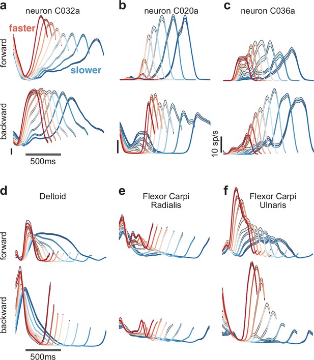
Speed-dependent neural and muscle activity patterns during cycling.
(a–c) Neural and (d–f) muscle activity across all eight speeds. Mean across-trial firing rate (or mean across-trial muscle activity) is plotted versus time for each speed bin. Envelopes give SEM across trials. Each panel plots activity for one example neuron or muscle. In each panel, data for forward cycling is plotted on top and data for backward cycling is plotted on bottom. All data is for monkey C. Traces are colored red to blue according to speed. All vertical calibrations for neural activity are 10 spikes/s. Muscle activity scale is arbitrary but preserved across all traces for a given muscle.
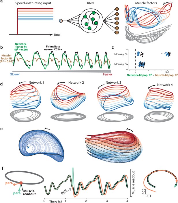
Goal-driven neural network solutions.
(a) Recurrent neural networks (RNNs) received a constant input whose level instructed cycling speed. Network-output targets were the top six muscle population factors (the projection of muscle population activity onto each of the top six PCs). Trajectories for the top three factors are plotted in state space, colored blue-to-red with increasing speed. Network outputs (not plotted for simplicity) were nearly identical to the target factors. (b) Example, for one neuron and all speeds, of fitting single-neuron activity with network factors (green) or muscle factors (brown). Fits were obtained by regressing the neuron’s activity against the top three factors (network or muscle). The R2 values shown here correspond to the example neuron. For the analyses below, we computed the population R2 across all neurons. The population R2 is the mean R2 across neurons, but taking into account response magnitudes (for example, a poor fit for a low-rate neuron has less impact). (c) Difference in population R2 for every network. The two cycling directions and two monkeys provided four network-output targets. For each we trained many networks. For each such network, the difference in population R2 for network-factor fits versus muscle-factor fits is plotted as a single point. The analysis was performed twice: once when fitting using two factors (black circles) and once when fitting using three factors (blue circles). Filled circles denote p<0.05 (paired one-tailed t-test with n=8 speeds) when testing whether network factors provided significantly better decoding than muscle factors. (d) Network trajectories for four example networks projected onto global PCs 1, 2, and 3 (the dominant dimensions across all speeds). Networks employ non-identical solutions due to different weight initializations before training. (e) Network trajectories are stable. Left: The network was perturbed so that it started at different initial states. All trajectories converge to the same limit cycle. Network input corresponded to the slow speed. Right: Same, but repeated for all eight input levels. Trajectories converge to an input-dependent limit cycle. (f) Using perturbations to explore network strategy. We delivered two perturbations to the network state. The rhythm-generation perturbation (orange) was designed to strongly impact activity in the plane containing the elliptical path (the plane defined by the top two PCs for the speed being examined) while remaining orthogonal to the muscle readout. The muscle-generation perturbation (green) was designed to do the opposite: strongly impact activity in one of the muscle readout dimensions while remaining orthogonal to the top two PCs. Traces versus time (middle) show network output with no perturbation (black), and the two perturbations (orange and green). State-space trajectories (right) plot network population activity in the top two PCs, which capture the dominant elliptical trajectory. Trajectories begin at the time of the perturbation. Consistent with its design, the muscle-generation perturbation had no immediate impact in this plane: the green trajectory begins in the same location as the black (unperturbed) trajectory. This reflects the fact that the muscle-generation perturbation had a large impact in other dimensions, but almost no influence on the future evolution of the elliptical trajectory. In contrast, the rhythm-generation perturbation had a large immediate impact on the elliptical trajectory, and permanently altered its phase: the orange trajectory ends at an earlier phase than the black trajectory, even though both are plotted for the same time-span.
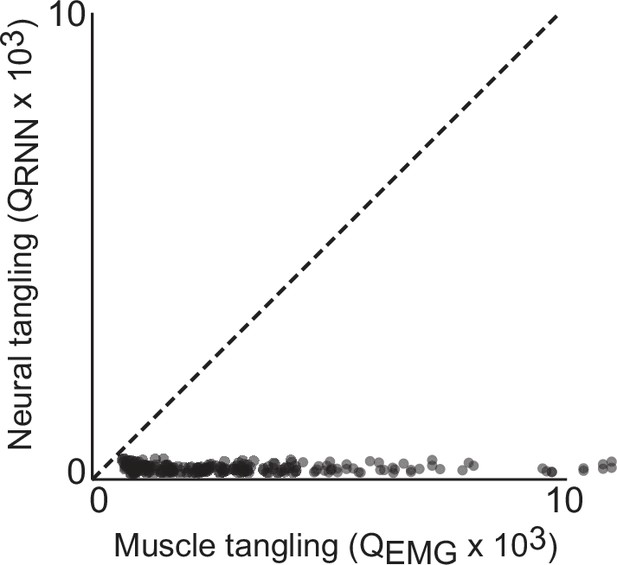
Trajectory tangling values for RNN trajectories vs EMG trajectories in the global (12 dimensional) subspace.
Each point shows tangling for one time point. Points are shown for all times during movement (sampled every 25ms) for all eight conditions. Black line indicates unity slope. Data are from one example network of the type shown in Figure 3a and d. Results are nearly identical across all networks of this type. Trajectory tanging was computed ‘globally’, both within and between different speeds.

Network trajectories for networks receiving input commands other than the graded-speed command used for the networks in Figure 3.
In all cases, target outputs were the same as in the original networks: the top six muscle-activity factors. (a) Illustration of networks that received forcing sinusoidal inputs: a sine and a cosine with the same period as the output targets. Example inputs are shown for slow (blue) and fast (red) cycling speeds. Each of these two inputs (the sine and cosine) was conveyed by a distinct input vector (inputs weight were initialized randomly). (b) Three example solutions for networks of this type, projected onto global PCs 1, 2, and 3. (c) Illustration of networks that received a distinct “one-hot encoded” input for each speed. The total number of inputs was equal to the number of trained speeds. Each input was conveyed by a distinct vector (initialized randomly, and thus close to orthogonal), with only one speed being ‘on’ for any given trial. (d) Three example network solutions for networks of this type.
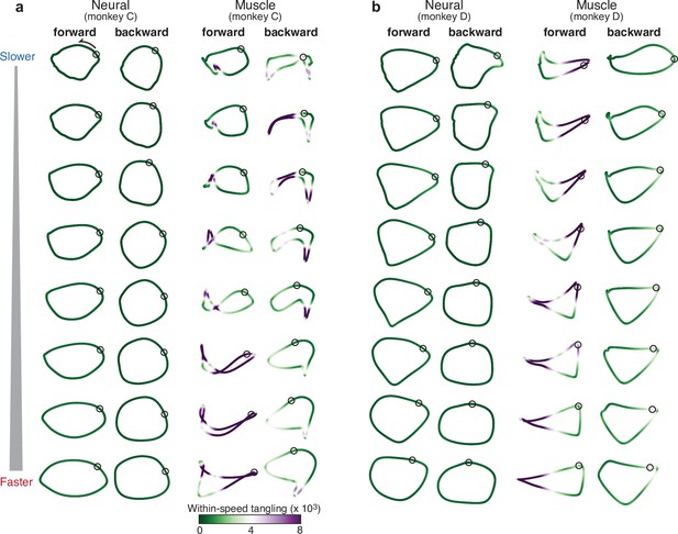
Comparison of individual-speed neural trajectories and muscle trajectories.
(a) Neural and muscle trajectories of monkey C. Trajectories were created by projecting the population response into the top two PCs, with PCs computed separately for each ‘condition’: that is, each speed bin and cycling direction. Each point within a trajectory corresponds to one time during the cycle for that condition. The time at which the pedal is at the top position is indicated by a black circle. Trajectories are shaded according to the instantaneous tangling value Q(t), computed for these two PCs and entirely within-speed (i.e. only tangling with other points within the same trajectory was considered). (b) Same analysis for monkey D.
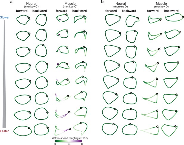
Same as Figure 4, but trajectory tangling was computed in the top six PCs.
As in Figure 4, both PCA and tangling considered only a single speed at a time.
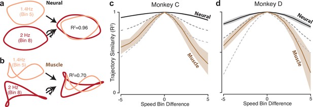
Path similarity between trajectories at different speeds.
(a) Method for calculating neural path similarity. Comparison involved two-dimensional neural trajectories (projected onto PCs 1 and 2) for different speed bins within the same cycling direction. One speed bin (here 1.4 Hz) was chosen as the ‘reference trajectory’. Its trajectory path was compared with the trajectory path for each other speed bin (2 Hz is shown for illustration). Comparison of trajectory similarity (computation of R2) followed reflection and rotation, selected to maximize similarity. (b) Same as panel (a) but for muscle data. (c) Average path similarity as a function of speed-bin difference between the reference trajectory and the trajectory with which it is compared. For example, for a speed-bin difference of two, the plotted R2 averages across all comparisons where the comparison trajectory differed from the reference trajectory by two speed bins. Shaded envelopes indicate the SEM. As noted above, the primary analyses compared paths in the top two PCs. For the neural data, we also compared paths in PCs 3 and 4 (dark dashed gray line) and PCs 5 and 6 (light dashed gray line). (d) Same as (c) but for monkey D.
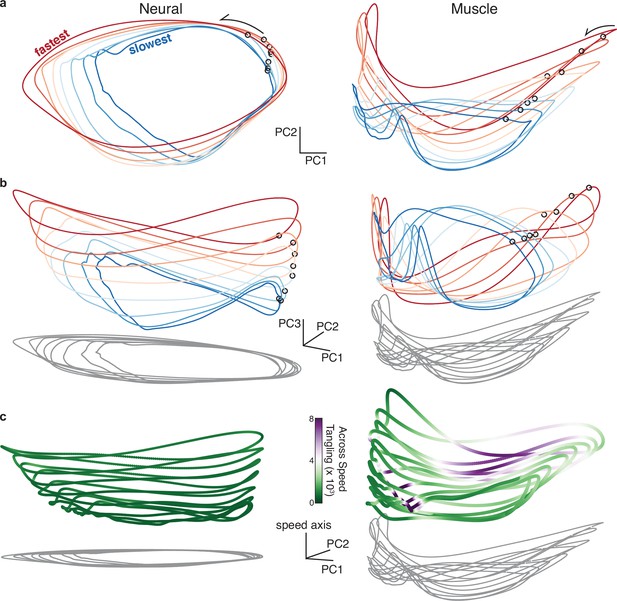
Neural and muscle population trajectories across speeds, with trajectories for every speed projected into a common basis.
All data are for monkey C, forward condition. (a) Neural and muscle activity projected onto global PCs 1 and 2: the dominant dimensions when PCA was applied across all speeds for that cycling direction (b) Same as (a) but for PCs 1, 2, and 3. (c) Same as (a) but for PCs 1, 2, and the ‘speed axis’ (see text for how this was found). Trajectories in (c) are colored according to instantaneous tangling values, considering only tangling across conditions and ignoring any within-condition tangling. Tangling was computed in a twelve-dimensional PC space, computed by applying PCA to the data for all speeds for a given direction.

Same as Figure 6 but for forward cycling for monkey D.
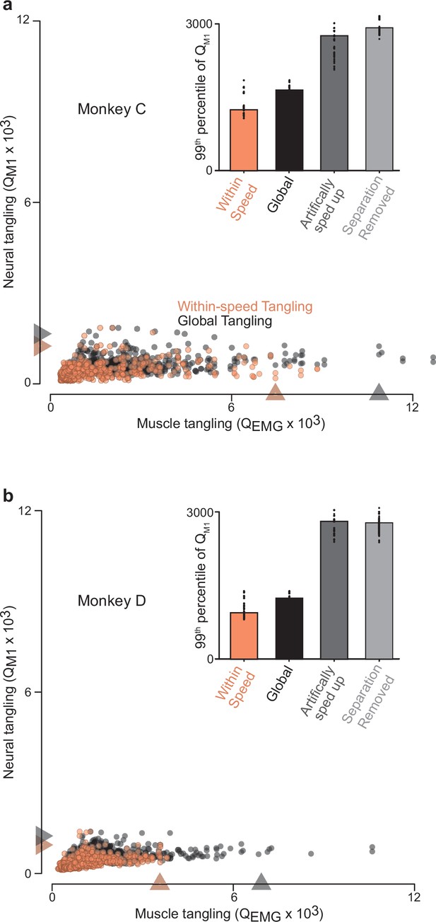
Trajectory tangling values for purely within-speed comparisons and global comparisons (within and across all speeds for a given direction).
(a) Scatterplot of neural-trajectory tangling versus muscle-trajectory tangling (monkey C) for within-speed tangling (orange) and global tangling (black). Each point shows tangling for one moment (one time during one speed and one direction). Points are shown for all times during movement (sampled every 25ms) for all sixteen conditions. Gray / orange triangles indicate 99th percentile tangling. All tangling values (both within-speed and global) were computed in the same twelve-dimensional global space found by applying PCA to all the data (that is, all speeds) for that cycling direction. The difference in the within-speed versus global computations simply involved whether the computation of tangling included only the trajectory for the speed containing a given state, or included all other trajectories. Note that, by construction, global tangling must be at least as high as within-speed tangling. Inset plots 99th percentile tangling values for within-speed tangling and global tangling. Also shown are values obtained by manipulating the empirical data to create new data without separation between speeds. For the ‘artificially sped up’ manipulation, all trajectories were identical in path but evolved according to their original rates. For the ‘separation removed’ manipulation, all trajectories were given the same mean and forced to unfold in the same dimensions. Black dots show 99th percentile tangling values for bootstrapped data (Materials and methods). (b) Same as (a) but for Monkey D.

Similar to insets in Figure 7, but ‘neural’ tangling assesses the population response of an example RNN rather than recorded population activity.
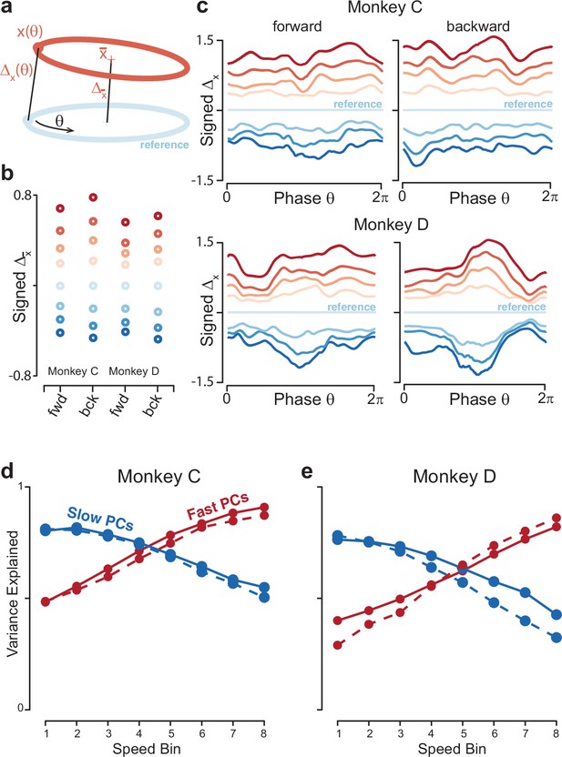
Quantification of separation between neural trajectories at different speeds.
(a) Illustration of the method for calculating distance as a function of phase. One speed bin was chosen to provide the reference trajectory. For the present analysis this was always speed bin 4, and the cartoon reference trajectory (light blue) is thus colored accordingly. We then took a trajectory from another speed bin (orange). We swept the phase, , of the reference trajectory, and for each phase computed the distance to the nearest point of the other trajectory. We also computed the distance between the trajectory means. (b) Distance between trajectory means, for each monkey and cycling direction. Speed bin 4 is the reference trajectory, and thus distance is zero. (c) Phase-dependent distance of the reference trajectory from each of the other trajectories. (d) Quantification of the degree to which elliptical trajectories unfold in the same set of dimensions across speeds. Slow PCs were the first two PCs based on speed bin 1, and fast PCs were the same based on speed bin 8. For each set of PCs, we computed the proportion of variance explained for each of the other speed bins. The analysis was performed separately for forward and backward cycling (solid and dashed lines, respectively). This analysis is repeated, using the top ten PCs, in Figure 8—figure supplement 2C, D. Data are for monkey C. (e) Same for monkey D.
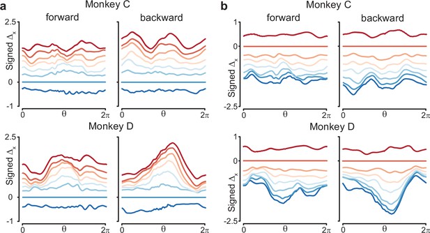
Similar to Figure 8c, but using different speed bins for the reference trajectory.
(a) Results when the trajectory in speed bin 2 was the reference trajectory. (b) Results when the trajectory in speed bin 7 was the reference trajectory.
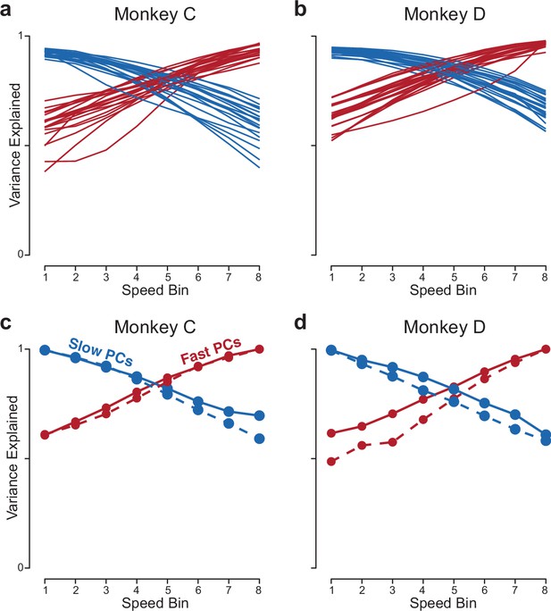
Analyses related to those in Figure 8d and e.
(a,b) Same as in Figure 8d and e, but the analysis is applied to the population response of RNNs (one line per trained network). (a,b) Same as in Figure 8d and e, but using more PCs (10 PCs, rather than 2).
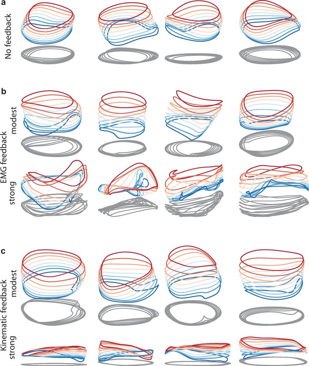
Network solutions with and without simulated sensory feedback.
Network inputs and outputs were as in Figure 3, except some networks were supplied with an additional input conveying delayed sensory feedback related to prior motor output. All examples were trained to produce outputs based on the muscle activity of Monkey C during forward cycling. Training occurred in the presence of all relevant inputs (including feedback if present). (a) Networks with no explicitly simulated sensory feedback (similar to Figure 3d). (b) Networks supplied with delayed EMG feedback (PCs 1–6 of muscle activity; 60ms delay) at a gain of 0.1 (top) and a gain of 10 (bottom). (c) Networks supplied with delayed kinematic feedback (horizontal and vertical position and velocity signals; 60ms delay) at a gain of 0.1 gain (top), and a gain of 10 (bottom).
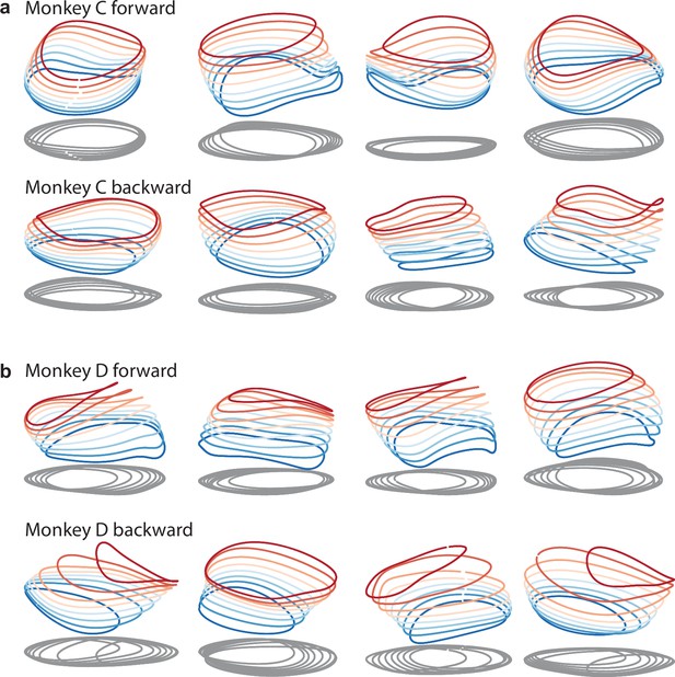
Same as in Figures 9a and 3d, but with additional example networks for the other cycling direction and the other monkey.
All networks are of the type illustrated in Figure 3a (a single input whose magnitude instructs speed). (a) Four networks trained to produce the muscle activity of monkey C during forward cycling (top row) and four networks trained to do the same for backward cycling (bottom row). (b) Same but for monkey D.


