Expansion and contraction of resource allocation in sensory bottlenecks
Figures
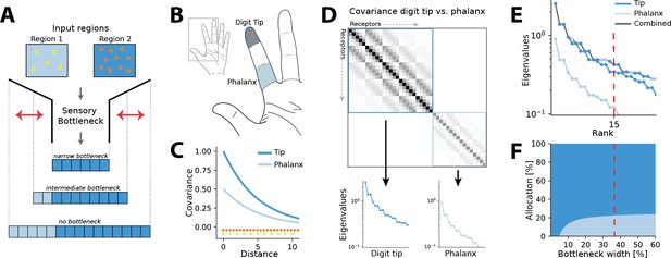
Illustration of the resource allocation problem and solution outline.
(A) Abstract problem setup. When two regions vary in their receptor densities and activation, how should a shared resource be allocated between them when that resource is limited, as in a sensory ‘bottleneck’? The allocation between the two regions may vary depending on the width of the bottleneck, for example, for narrow bottlenecks it might be most efficient to allocate all resources to the higher density region 2. (B) Application of the problem to the tactile system. The density of touch receptors differs across regions of the hand (e.g. fingertip, shown in orange, versus finger phalanx, yellow). Different finger regions make contact with objects at different rates (dark blue versus light blue shading, darker colours indicating higher contact rates). (C) Sensory inputs are correlated according to a covariance function that decays with distance between receptors on the sensory sheet. This function is evaluated at different receptor distances depending on the density of sensory receptors (orange versus yellow dots at the bottom). Regions with higher probability of activation exhibit greater variance (dark versus light blue curves). (D) Decorrelation of sensory inputs in the presence of a bottleneck is achieved by calculating and retaining the eigenvectors and eigenvalues of the receptor covariance matrix. Here, this matrix is approximated as a block matrix, which allows calculating the eigenvalues for each region individually (dark blue versus light blue box). (E) The combined set of eigenvalues from all regions is then sorted; the region where each successive eigenvalue in the combined sorted set originates from determines where that output neuron’s receptive field will fall. (F) Counting which input regions successive eigenvalues belong to results in the allocation breakdown for different bottlenecks. For certain forms of the covariance function, this allocation can be calculated analytically.
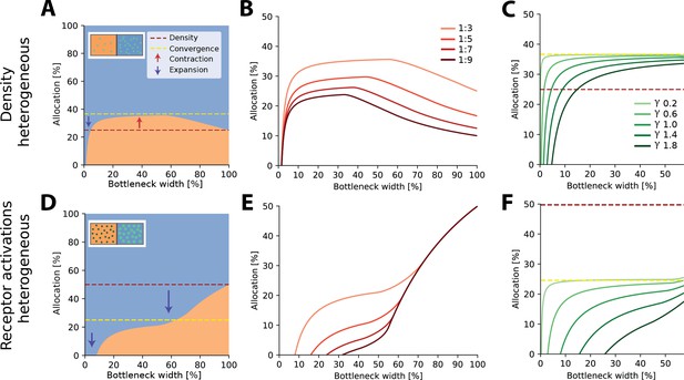
Optimal resource allocation for heterogeneous receptor densities or input statistics leads to complex trade-offs.
(A) Illustration of resource allocation for heterogeneous receptor density but homogeneous stimulus statistics over all bottleneck sizes. Orange denotes the lower density region and blue the higher density region, with a ratio of 1:3. Dotted lines show proportional representation according to receptor numbers (red) and convergence of the optimal allocation in the limit (yellow). Arrows indicate contraction (up) and expansion (down) of the higher density region representation. Inset demonstrates change in density between the regions. (B) Bottleneck allocation boundaries for different density ratios (given as low:high). The area below each line corresponds to the low-density representation, while the area above corresponds to the high-density representation, as in (A). (C) Effect of changing the extent of the spatial correlations (parameterized by the decay value γ, see ‘Methods’ for details and Figure 2—figure supplement 1 for an illustration of the covariance function for different values of γ). Density ratio is set at 1:3 for all γ. Increasing γ leads to expansion of the higher density region for a larger initial portion of the bottleneck. (D–F) Same as in row above but for homogeneous density and heterogeneous receptor activation ratios. (D) Illustrative example with the blue region having higher receptor activation. Note that the representation of the higher activation region is expanded for all bottleneck widths. Inset demonstrates difference in activation between the regions. Larger, brighter coloured points indicate higher activation for that region compared to the other. (E) Allocation boundaries for different activation ratios. The representation of the higher activation regions is expanded for all bottlenecks. As activation ratio increases, the highly active region allocation is expanded for wider bottlenecks. (F) Changing the extent of spatial correlations (γ) has larger effects when the activation ratio is heterogeneous (set at 1:3 for all γ) compared to heterogeneous density (C). See Figure 2—figure supplement 2 for an equivalent figure considering 1D receptor arrangements.
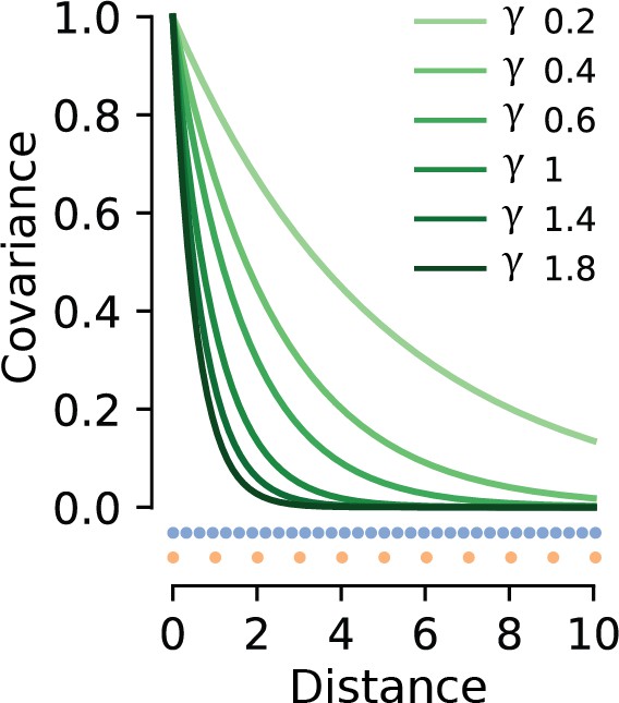
Effect of different values of γ on the covariance function decay.
Smaller γ leads to a slower decay and therefore a larger extent of spatial correlations. When the sigma is large, receptors have less similar responses to their neighbours, and therefore co-vary less. Orange points denote the baseline spacing of receptors along one dimension. When receptor density is varied, the other region will have higher density (e.g. 1:3, indicated by blue dots).
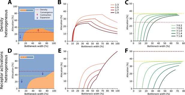
Resource allocation for heterogeneous receptor densities and variations in input statistics in 1D.
(A) Examples of allocation for two input regions with differing receptor densities and activation (see insets) for different bottleneck widths, demonstrating complex trade-offs in resource allocation. Here, ratio for low:high density = 1:3, γ=1. Dotted lines show representation proportional to receptor density (red) and convergence in the limit (yellow). Arrows indicate expansion (down) and contraction (up) of the higher density (blue) region. Both expansion and contraction of the higher density region are seen, similar to the 2D case. (B). Allocation boundaries for different density ratios. Ratios are given as low:high density. (C) Effect of changing the decay γ parameter. Density ratio is set at 1:3 for all sigmas. (D–F), same as above but for density constant across the two regions and receptor activation manipulated. Activation ratio is set at 1:3 in (D, F). Note that in (D) the representation of the higher activation (blue) region is expanded for all bottlenecks.
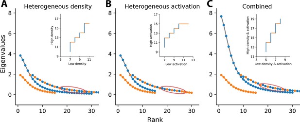
Illustration of eigenvalue sorting and resulting allocation.
Main panels: eigenvalues for heterogeneous density (A), heterogeneous activation (B), or combined (C). For each, the manipulated ratio is set as 1:2. For simplicity, the example considers 1D regions. Orange markers show eigenvalues from the baseline region, which is identical for all panels. Blue markers show eigenvalues from the second region with higher density, activation, or both, respectively. Markers connected by the grey line show the combined set of sorted eigenvalues from both regions. Insets: cumulative allocation for the set of eigenvalues marked by the red ellipse in the main panel. Horizontal orange lines indicate eigenvalues from and therefore allocation to the orange region, whilst vertical blue lines indicate allocation to the blue region. (A) Heterogeneous density. Increased receptor density in the blue region causes higher spatial correlations between neighbouring receptors and therefore larger eigenvalues, leading to a scaling of the eigenvalue curve. Increased density also leads to a larger number of receptors in the blue region, increasing the number of eigenvalues from this region and the total number of eigenvalues considered. (B) Heterogeneous activation. Increased variance in the blue region leads to a scaling of the eigenvalue curve. However, the number of receptors in the blue region is not affected, explaining differences observed compared to (A). (C) Heterogeneous density and activation. Effects from (A) and (B) are combined, leading to a double scaling of the eigenvalue curve, plus an increase in the total number of eigenvalues.
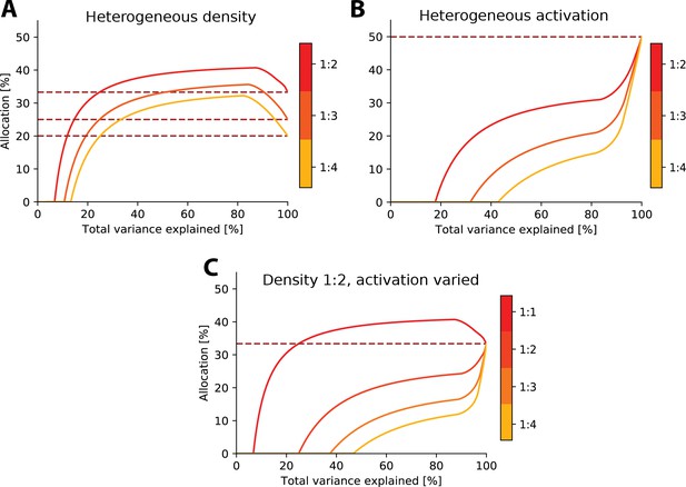
Limit on information rather than number of neurons.
Resource allocations where the bottleneck is expressed as variance explained. Because eigenvalues decrease dramatically in size, this re-expression results in a ’squashing’ of the allocation curve towards higher bottleneck sizes as the initial eigenvalues in the sorted set explain a much larger amount of the variance. (A) Examples with heterogeneous density. (B) Examples with heterogeneous activation. (C) Examples with heterogeneous density and activation. Dashed red line in each denotes allocation proportional to density.
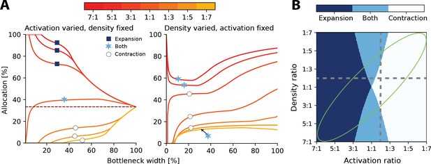
Interactions between heterogeneous statistics and density.
(A) Allocations with both heterogeneous density and activation ratios. Expansion and contraction for a baseline region where relative density and activation is varied over the other region. All ratios given are baseline:other region. Left: fixed density ratio of 1:2, while activation ratio is varied between 7:1 and 1:7 (see colourbar). Purple dashed line indicates allocation proportional to density ratio. Right: fixed activation ratio of 1:2, while density ratio is varied between 7:1 and 1:7. The coloured markers indicate whether the baseline region is expanded (dark blue squares), contracted (white circles), or both (light blue stars) across all bottlenecks. (B) Possible expansion/contraction regimes for the baseline region based on combinations of density and activation ratios. Colours as shown by the markers in (A). Grey dashed lines show all possible allocation regimes for an example with either fixed density ratio (horizontal, corresponding plot in A, left) or activation ratio (vertical, A, right). When activation is fixed and density is varied, the allocations can be either expanded/both or contracted/both across the full bottleneck width. In contrast, when the density ratio is fixed and activation is varied, the allocation of a region could be any of the three regimes. The green ellipse highlights parameter combinations where activation and density ratios are correlated. See Figure 3—figure supplement 1 for a comparison of how receptor density and activation interact between 1D and 2D receptor arrangements.
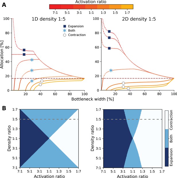
Comparison between 1D and 2D results for heterogeneous activation and density.
(A) Effect of changing both the density and activation ratios, and possible resource allocations for two regions. Plots show the same density ratio, 1:5, considering 1D (left) and 2D (right) regions. Allocation % is for baseline region (region 1). Each line denotes the variance ratios between region 1:region 2 (see colourbar). Solid lines denote contraction of baseline region representation, whilst dotted lines are expansion. The horizontal red dashed line shows the proportional density representation. Across both 1D and 2D, different patterns of expansion and contraction occur. The baseline region is more likely to either be fully expanded or contracted for the whole bottleneck in 2D, whereas in 1D both expansion and contraction occur (denoted by light blue star, which covers three activation ratios in 1D, but only 1:1 in 2D as indicated by the markers). In 1D, the same activation and density ratio leads to convergence at the proportional density, whereas for 2D, the convergence is always lower. (B) Comparison of the possible allocation schemes between 1D (left) and 2D (right). Dotted grey line denotes density ratio from (A). In 2D, the likelihood of both expansion and contraction (light blue region) of the representations decreases.
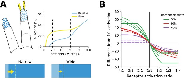
Re-allocation to account for changes in stimulus statistics.
(A) Top left: illustration of problem setup. Increased stimulation is applied to the middle digit (yellow symbols), leading to changes in optimal allocations. Top right: optimal allocations for baseline (blue) and stimulation (yellow) conditions across all bottleneck widths. Stimulation of the middle finger increases its representation, but the relative magnitude of the effect depends on the bottleneck width. Bottom: changes in allocation of the middle digit for two bottleneck widths (indicated by dashed lines above). The increase is proportionally larger for the narrow compared to the wide bottleneck. (B) Change in allocation when receptor activation for an input region increases (left half) or decreases (right half). Drastic changes in cortical allocation are observed for narrow bottlenecks (green lines), while wider bottlenecks (red and purple lines) induce only moderate change. Solid lines denote equal receptor density across both regions, while dashed lines show examples with varying density.

Allocations for other monotonically decreasing covariance functions.
(A) Three covariance functions of different smoothness taken from the Matérn class, differing in the parameter ν (see ‘Methods’). (B) Examples of numerically determined allocation for the covariance functions shown in (A) for two scenarios. Left: density ratio 1:2, equal activation. Right: density ratio 1:6, activation ratio 1:3. The red dashed line shows the analytic solution for the negative exponential covariance (). (C) Estimated allocations at convergence for different density ratios (horizontal axis) and a fixed activation ratio of 1:2. Solid lines denote numerical convergence, and dashed lines refer to fitted functions (see main text).

Resource allocation in the star-nosed mole.
(A) Star-nosed moles have two sets of 11 tactile rays used for detecting and capturing prey. (B) Fibre innervation densities for each ray. (C) Typical usage percentages for each ray during foraging. Higher usage corresponds to greater average activation of receptors located on the corresponding ray. Typically prey is funnelled from distal rays towards ray 11, which is located next to the mouth. Ray outlines adapted from Catania et al., 2011. (D) Left: explained variance () between model predictions and cortical allocation for three different models: restricted to receptor density only (purple), restricted to receptor activation only (green), and a full model (pink) that incorporates accurate values for both factors. Results confirm previous findings that ray usage is a better predictor of cortical allocation than receptor densities alone. Additionally, we show that including both of these factors provides a marginal improvement to the fit, with the highest (86%). Right: predicted versus empirical cortical allocations for all rays. When including both density and activation parameters, the model provides a good fit to empirical measurements. Scatter plots for all models are available in Figure 6—figure supplement 1B. (A) Reproduced from Figure 1C in Catania et al., 2011, copyright Kenneth Catania.
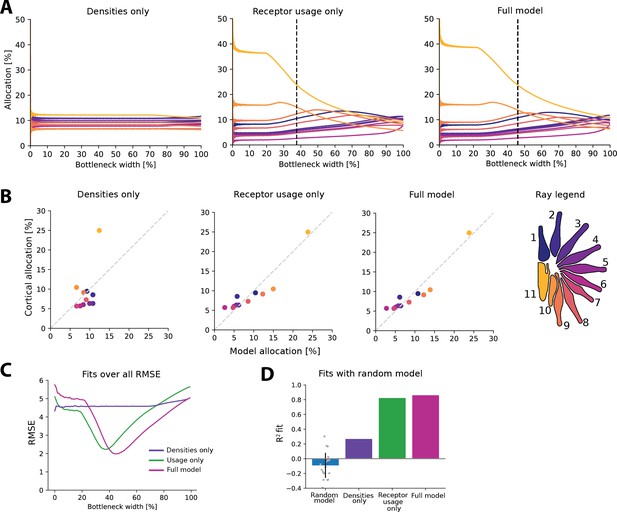
Additional figures for the star-nosed mole.
(A) Fits across all bottleneck sizes for each model. Lowest root-mean-square error (RMSE) is indicated for each model. Dashed line indicates lowest RMSE (excluded for densities-only model as RMSE is fairly constant across bottlenecks, see C). (B) Corresponding fits at each selected bottleneck size compared to cortical data. (C) RMSE values over all bottleneck sizes for each model. (D) Can any values be fit given the range of bottleneck sizes? Here, we test whether a good fit can be obtained for a series of ‘random models’, where the random values are selected for each ray’s density and variance within the range of parameters. The same fitting process is then applied, where the lowest RMSE fit to the cortical data is selected based on the range of possible bottlenecks. Note that values are calculated with fixed intercept, resulting in some negative values. Most random models perform poorly, suggesting that the model cannot be fit successfully without using the precise parameter values from the empirical star-nosed mole data.
Tables
Model parameters for the star-nosed mole.
| Ray | 1 | 2 | 3 | 4 | 5 | 6 | 7 | 8 | 9 | 10 | 11 |
|---|---|---|---|---|---|---|---|---|---|---|---|
| Size | 1.14 | 1.21 | 1.21 | 1.17 | 1.08 | 1.02 | 1.00 | 1.13 | 1.05 | 0.87 | 1.10 |
| Density | 45.78 | 47.14 | 45.82 | 45.69 | 45.2 | 46.91 | 43.3 | 44.01 | 44.26 | 47.92 | 50.46 |
| Activation | 0.03 | 0.01 | 0.02 | 0.01 | 0.02 | 0.01 | 0.02 | 0.02 | 0.04 | 0.08 | 0.11 |
| γ | 0.99 | 1.00 | 1.02 | 1.01 | 1.00 | 1.01 | 0.99 | 1.04 | 1.10 | 1.16 | 1.27 |


