Imaging of the pial arterial vasculature of the human brain in vivo using high-resolution 7T time-of-flight angiography
- Athinoula A. Martinos Center for Biomedical Imaging, Massachusetts General Hospital, United States
- Department of Radiology, Harvard Medical School, United States
- Centre for Advanced Imaging, The University of Queensland, Australia
- Department of Biomedical Magnetic Resonance, Institute of Experimental Physics, Otto-von- Guericke-University, Germany
- High Field MR Centre, Department of Biomedical Imaging and Image-guided Therapy, Medical University of Vienna, Austria
- Karl Landsteiner Institute for Clinical Molecular MR in Musculoskeletal Imaging, Austria
- Department of Neurology, Medical University of Graz, Austria
- German Center for Neurodegenerative Diseases, Germany
- Center for Behavioral Brain Sciences, Germany
- Leibniz Institute for Neurobiology, Germany
- Division of Health Sciences and Technology, Massachusetts Institute of Technology, United States
Figures
Figure 1
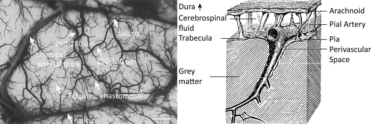
Properties of the pial arterial vasculature of the human brain.
Left: The pial vascular network on the medial orbital gyrus depicted using intravascular India ink injection (adapted with permission from Duvernoy, 1999; this is not covered by the CC-BY 4.0 license and further reproduction of this panel would need permission from the copyright holder). The arrows indicate the average diameter of central pial arteries (260–280 μm), peripheral pial arteries (150–180 μm), and pial arterioles (<50 μm). Pial anastomoses are commonly formed by arteries ranging from 25 to 90 μm in diameter. For reference, the diameter of intracortical penetrating arterioles is approximately 40 μm (scale bar: 2.3 mm). Right: Pia-arachnoid architecture (adapted with permission from Ranson and Clark, 1959; this is not covered by the CC-BY 4.0 license and further reproduction of this panel would need permission from the copyright holder) illustrates the complex embedding of pial vessels, which are surrounded by various membrane layers that form the blood-brain barrier, cerebrospinal fluid, and grey matter (Marin-Padilla, 2012; Mastorakos and McGavern, 2019; Ranson and Clark, 1959).
© 1959, Springer. W. B. Saunders Company Permissions: The left part of Figure 1 is adapted from Duvernoy, 1999, and the right side of Figure 1 is adapted from Ranson and Clark, 1959. Relevant permission have been obtained from the publishers. These are not covered by the CC-BY 4.0 license and further reproduction of this panel would need permission from the copyright holder
Figure 2
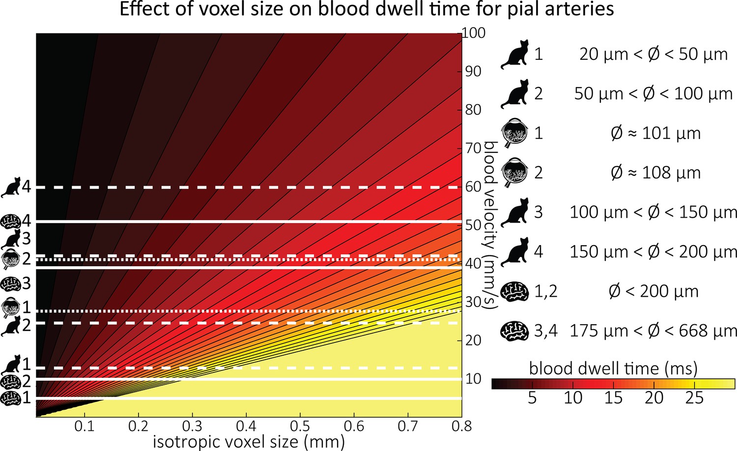
Blood dwell time (ms) as a function of blood velocity and voxel size.
For small voxel sizes, blood dwell times are short even for low blood velocities. The horizontal white lines indicate blood velocities reported in humans (solid lines) in the centrum semiovale (1 and 2) and the basal ganglia (3 and 4) (Bouvy et al., 2016), in cats (dashed lines) for various pial artery diameters (Kobari et al., 1984), and human retina (dotted lines) (Nagaoka and Yoshida, 2006). For reference, red blood cells in the capillaries are estimated to move at approximately 1 mm/s (Cipolla, 2009; Wei et al., 1993), whereas blood velocities in the major cerebral arteries can reach 1000 mm/s (Lee et al., 1997; Molinari et al., 2006).
Figure 3 with 1 supplement
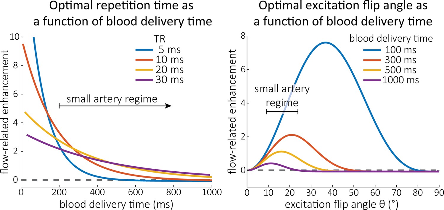
Optimal imaging parameters for small arteries.
:Left: Flow-related enhancement (FRE) was simulated as a function of blood delivery time for different repetition times assuming an excitation flip angle of 18° and longitudinal relaxation times of blood and tissue of 2100 and 1950 ms at 7 Tesla (T), respectively. Overall, FRE decreases with increasing blood delivery times. In the small vessel regime, that is, at blood delivery times >200 ms, longer repetition times result in higher FRE than shorter repetition times. Right: FRE was simulated as a function of excitation flip angle for different blood delivery times assuming a value of 20 ms and longitudinal relaxation rates as above. The excitation flip angle that maximizes FRE for longer blood delivery times is lower than the excitation flip angle that maximizes FRE for shorter blood delivery times, and often the optimal excitation flip angle is close to the Ernst angle for longer blood delivery times (Ernst angle: 8.2°; optimal excitation flip angles: 37° (100 ms), 21° (300 ms), 16° (500 ms), 11° (1000 ms)).
Figure 3—figure supplement 1
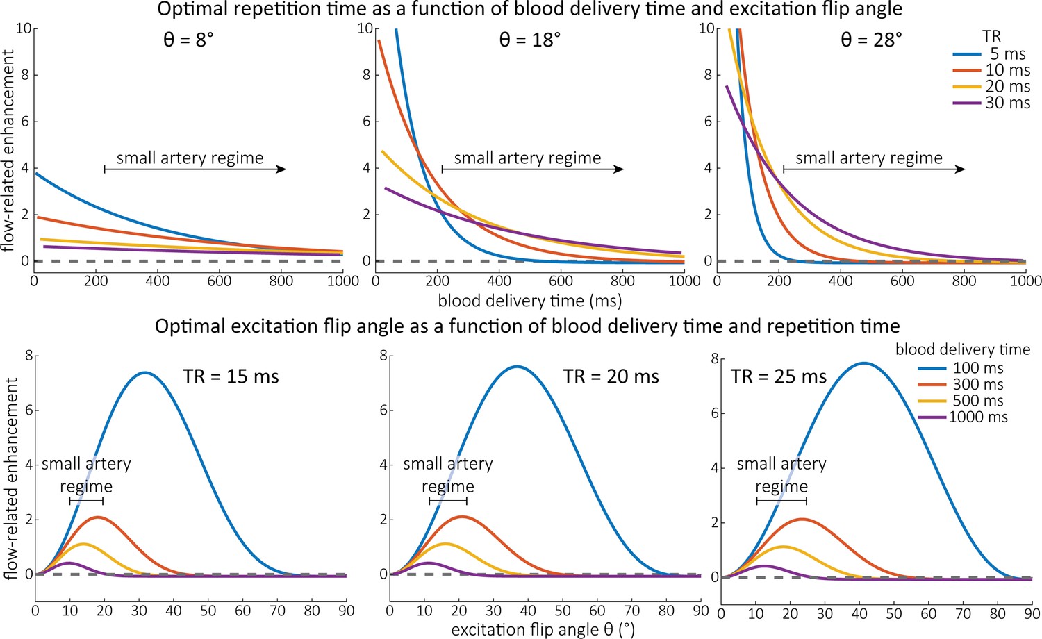
Optimal imaging parameters for small arteries.
This assessment follows the simulations presented in Figure 3, but in addition shows the interdependency for the corresponding third parameter (either flip angle or repetition time). Top: Flip angles close to the Ernst angle show only a marginal flow-related enhancement; however, the influence of the blood delivery time decreases further (left). As the flip angle increases well above the values used in this study, the flow-related enhancement in the small artery regime remains low even for the longer repetition times considered here (right). Bottom: The optimal excitation flip angle shows reduced variability across repetition times in the small artery regime compared to shorter blood delivery times.
Figure 4 with 2 supplements
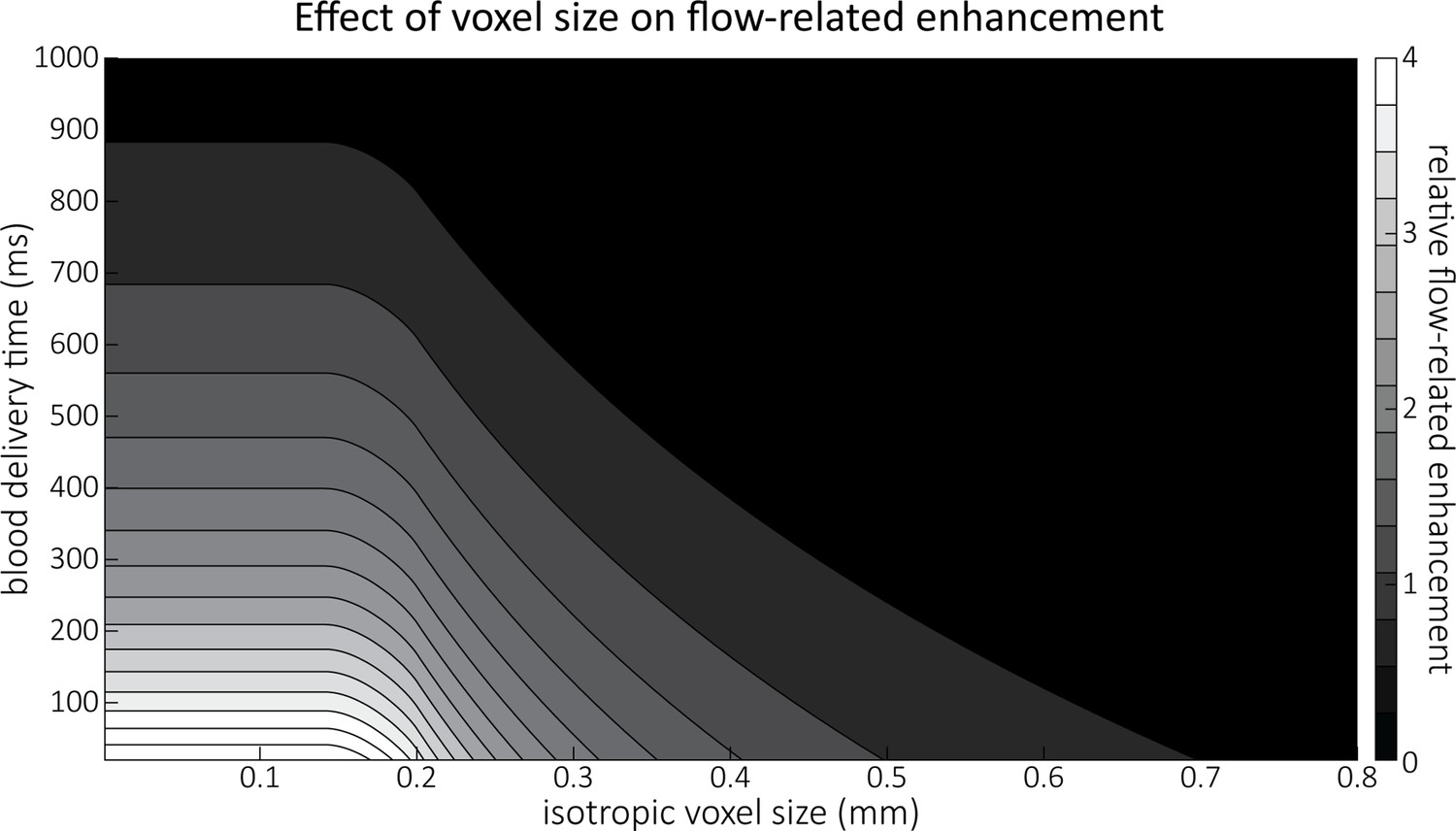
Effect of voxel size and blood delivery time on the relative flow-related enhancement (FRE), assuming a pial artery diameter of 200 μm.
The relative FRE represents the signal intensity in the voxel containing the artery relative to the surrounding tissue (Equation (3)). For example, an FRE of 0 would indicate equal intensity, and an FRE of 1 would indicate twice the signal level in the voxel compared to the surrounding tissue. The FRE decreases with blood delivery time due to more signal attenuation (Equation (2)) and with voxel size due to more partial-volume effects (Equation (4)).
Figure 4—figure supplement 1
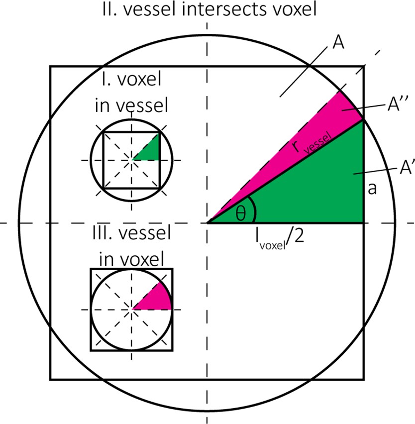
Estimation of the blood volume fraction for case (I) voxel in vessel, case (II) vessel intersects voxel, and case (III) vessel in voxel.
The pink regions indicate circular sectors and the green regions indicate right triangles. The full split into the 8 equal areas is shown for cases (I) and (III), the partial areas and are shown for case (II).
Figure 4—figure supplement 2
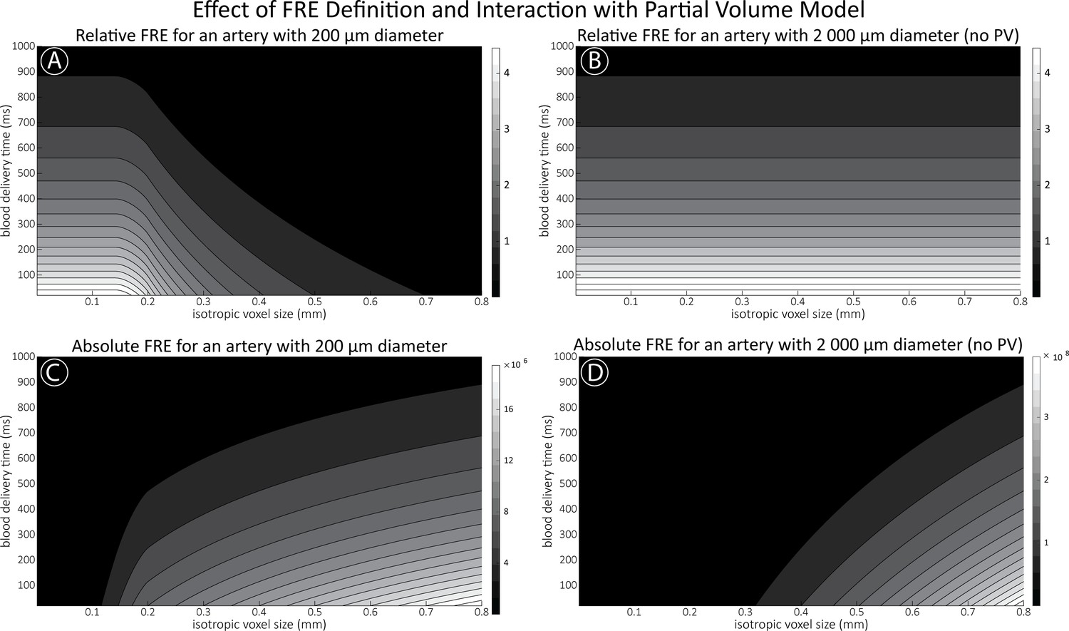
Effect of voxel size and blood delivery time on the relative flow-related enhancement (FRE) using either a relative (A,B) (Equation (3)) or an absolute (C,D) (Equation (12)) FRE definition assuming a pial artery diameter of 200 μm (A,C) or 2000 µm, that is, no partial-volume effects at the central voxel of this artery considered here.
Figure 5 with 1 supplement
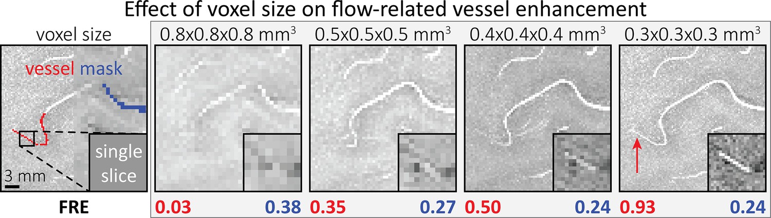
Effect of voxel size on flow-related vessel enhancement.
Thin axial maximum intensity projections containing a small artery acquired with different voxel sizes ranging from 0.8 to 0.3 mm isotropic are shown. The flow-related enhancement (FRE) is estimated using the mean intensity value within the vessel masks depicted on the left, and the mean intensity values of the surrounding tissue. The small insert shows a section of the artery as it lies within a single slice. A reduction in voxel size is accompanied by a corresponding increase in FRE (red mask), whereas no further increase is obtained once the voxel size is equal or smaller than the vessel size (blue mask).
Figure 5—figure supplement 1
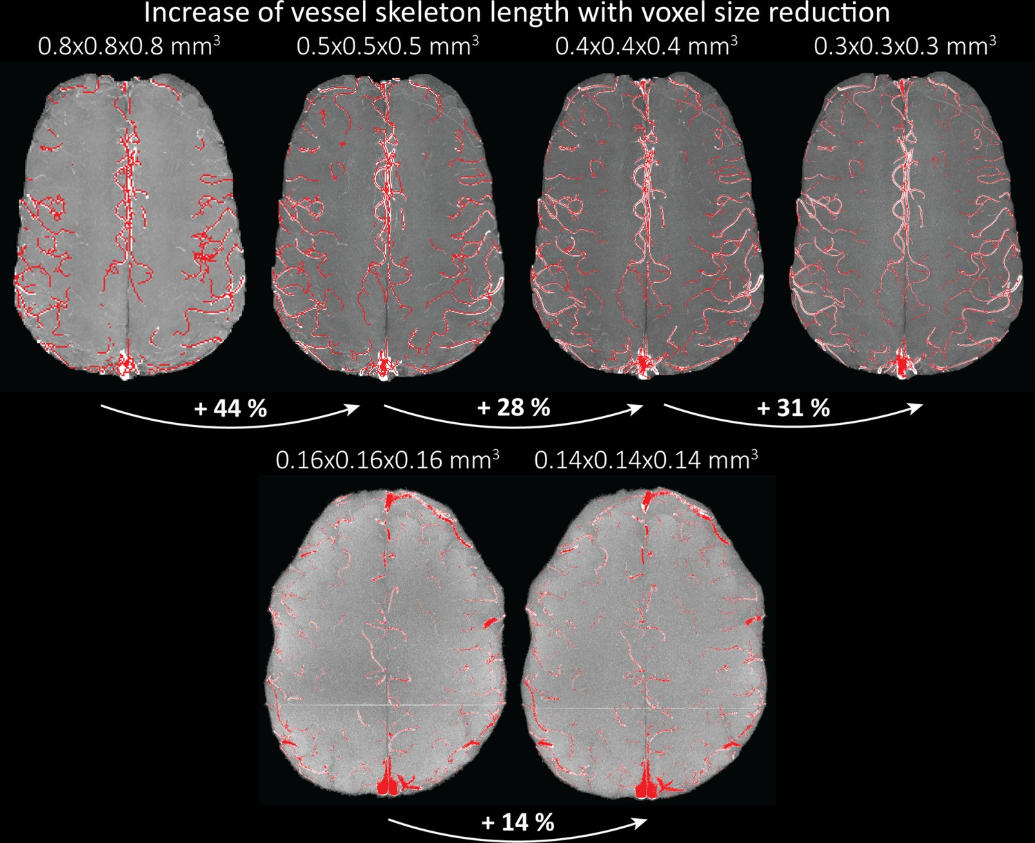
Increase of vessel skeleton length with voxel size reduction.
Axial maximum intensity projections for data acquired with different voxel sizes ranging from 0.8 to 0.3 mm (top) (corresponding to Figure 5) and 0.16 to 0.14 mm isotropic (corresponding to Figure 7) are shown. Vessel skeletons derived from segmentations performed for each resolution are overlaid in red. A reduction in voxel size is accompanied by a corresponding increase in vessel skeleton length.
Figure 6 with 5 supplements
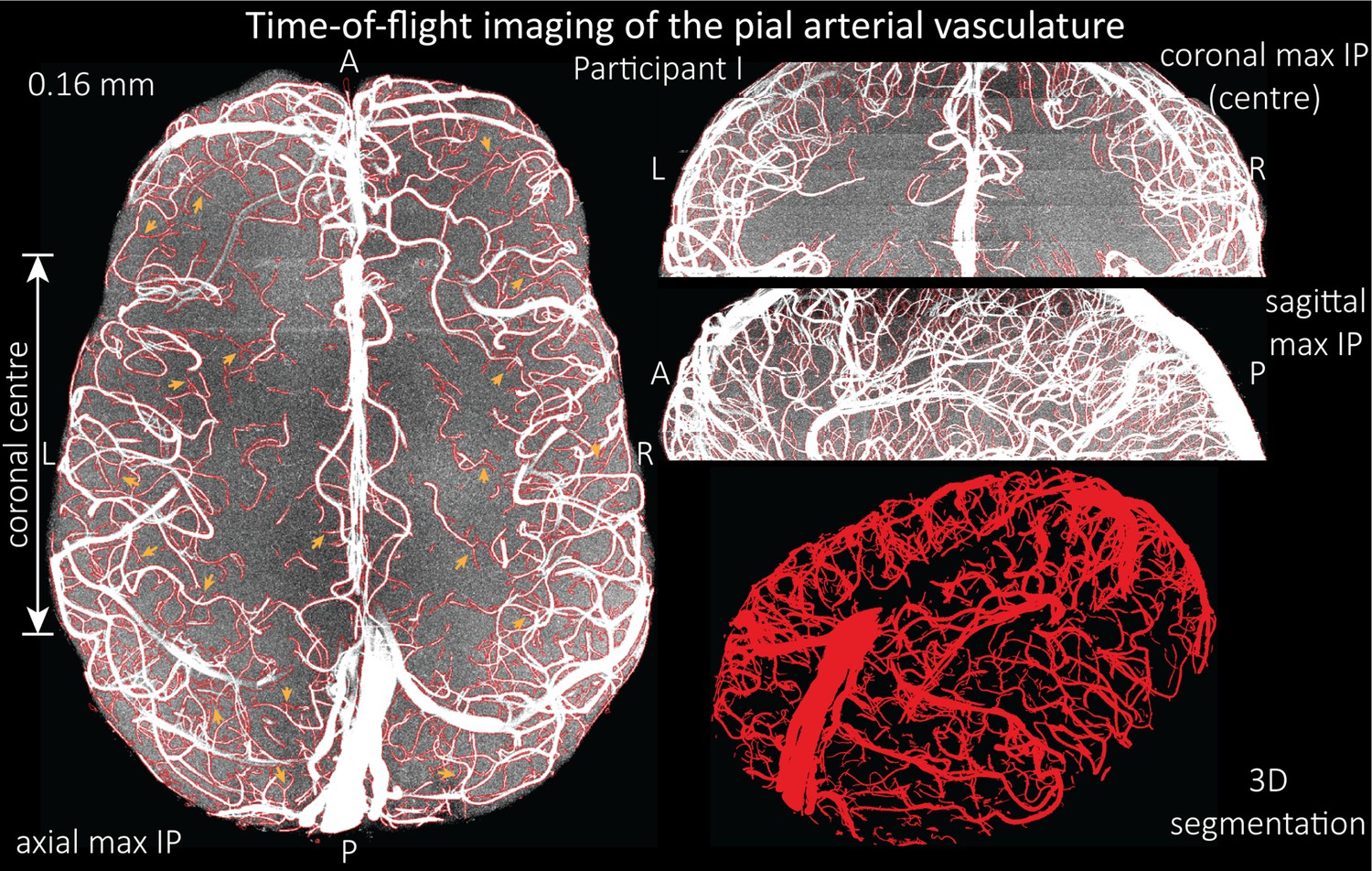
Time-of-flight imaging of the pial arterial vasculature at 0.16 mm isotropic resolution and 50 mm coverage in the head-foot direction.
Left: Axial maximum intensity projection and outline of the vessel segmentation overlaid in red. Examples of the numerous right-angled branches are indicated by orange arrows. Right: Coronal maximum intensity projection and segmentation of the central part of the brain (top), sagittal maximum intensity projection and segmentation (middle), and 3D view of the vessel segmentation (bottom).
Figure 6—figure supplement 1
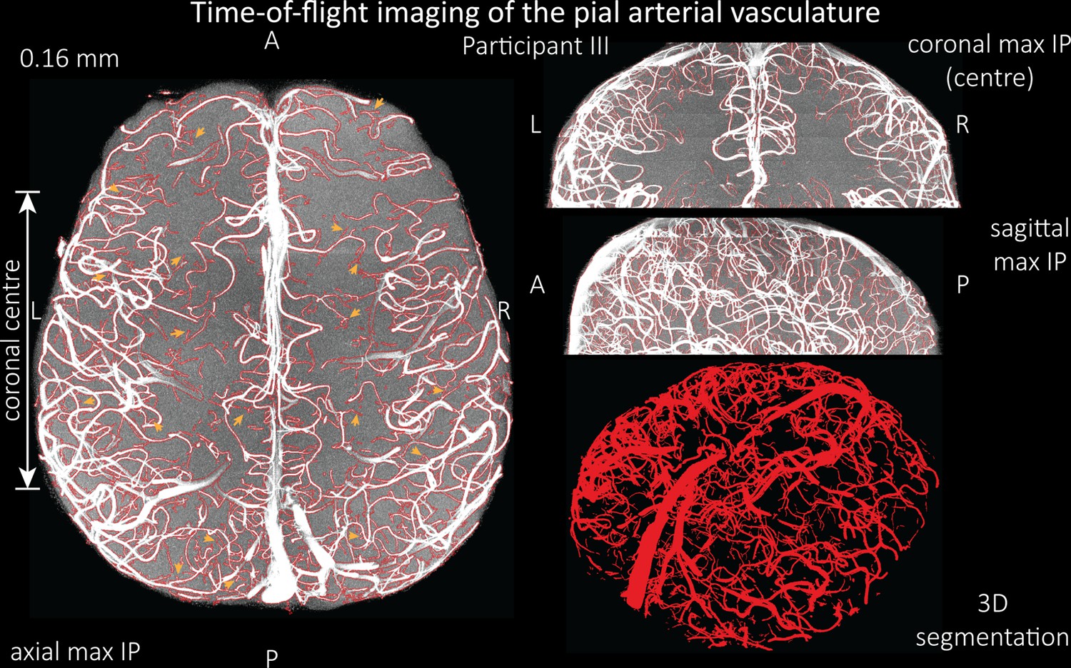
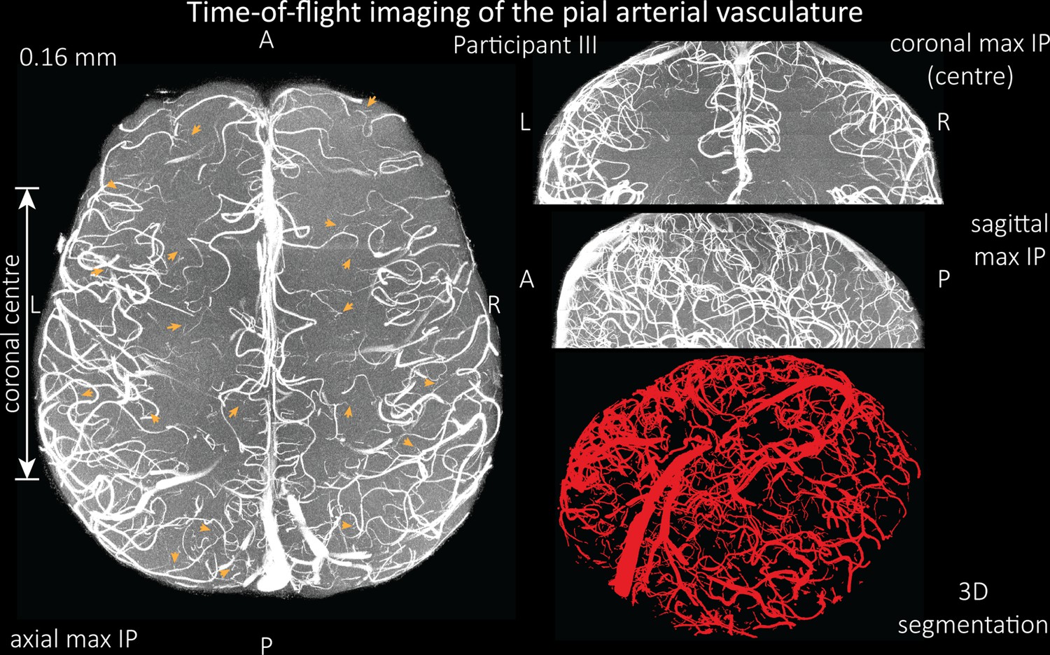
Time-of-flight imaging of the pial arterial vasculature at 0.16 mm isotropic resolution and 58 mm coverage in the head-foot direction showing the results from participant III using the same acquisition protocol as for Figure 6.
Left: Axial maximum intensity projection and outline of the vessel segmentation overlaid in red. Examples of the numerous right-angled branches are indicated by orange arrows. Right: Coronal maximum intensity projection and segmentation of the central part of the brain (top), sagittal maximum intensity projection and segmentation (middle), and 3D view of the vessel segmentation (bottom).
Figure 6—figure supplement 2
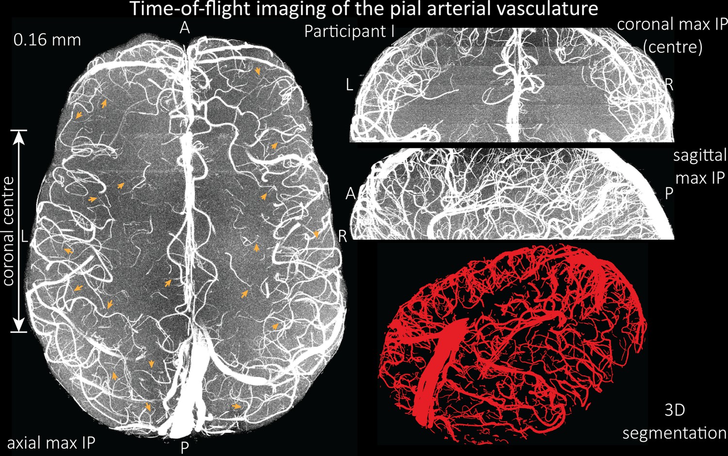
Time-of-flight imaging of the pial arterial vasculature at 0.16 mm isotropic resolution and 50 mm coverage in the head-foot direction showing the same data of participant I as in Figure 6, but without the overlay of the segmentation.
Left: Axial maximum intensity projection. Examples of the numerous right-angled branches are indicated by orange arrows. Right: Coronal maximum intensity projection of the central part of the brain (top), sagittal maximum intensity projection (middle), and 3D view of the vessel segmentation (bottom).
Figure 6—figure supplement 3
Time-of-flight imaging of the pial arterial vasculature at 0.16 mm isotropic resolution and 58 mm coverage in the head-foot direction showing the same data of participant III as in Figure 6—figure supplement 1 but without the overlay of the segmentation.
Left: Axial maximum intensity projection. Examples of the numerous right-angled branches are indicated by orange arrows. Right: Coronal maximum intensity projection of the central part of the brain (top), sagittal maximum intensity projection (middle), and 3D view of the vessel segmentation (bottom).
Figure 6—video 1
Video of the segmentation of the time-of-flight data acquired with 160 µm isotropic voxel size as shown in Figure 6.
Figure 6—video 2
Video of the segmentation of the time-of-flight data acquired with 160 µm isotropic voxel size as shown in Figure 6—figure supplement 1.
Figure 7 with 4 supplements
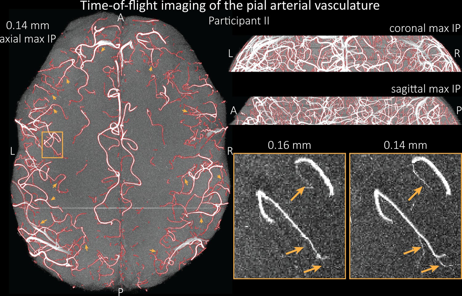
Time-of-flight imaging of the pial arterial vasculature at 0.14 mm isotropic resolution and 19.6 mm coverage in the foot-head direction.
Left: Axial maximum intensity projection and outline of the vessel segmentation overlaid in red. Examples of the numerous right-angled branches are indicated by orange arrows. Right: Coronal maximum intensity projection and segmentation (top) and sagittal maximum intensity projection and segmentation (middle). A comparison of 0.16 and 0.14 mm voxel size (bottom) shows several vessels visible only at the higher resolution. The location of the insert is indicated on the axial maximum intensity projection on the left. Note that for this comparison, the coverage of the 0.14 mm data was matched to the smaller coverage of the 0.16 mm data.
Figure 7—figure supplement 1
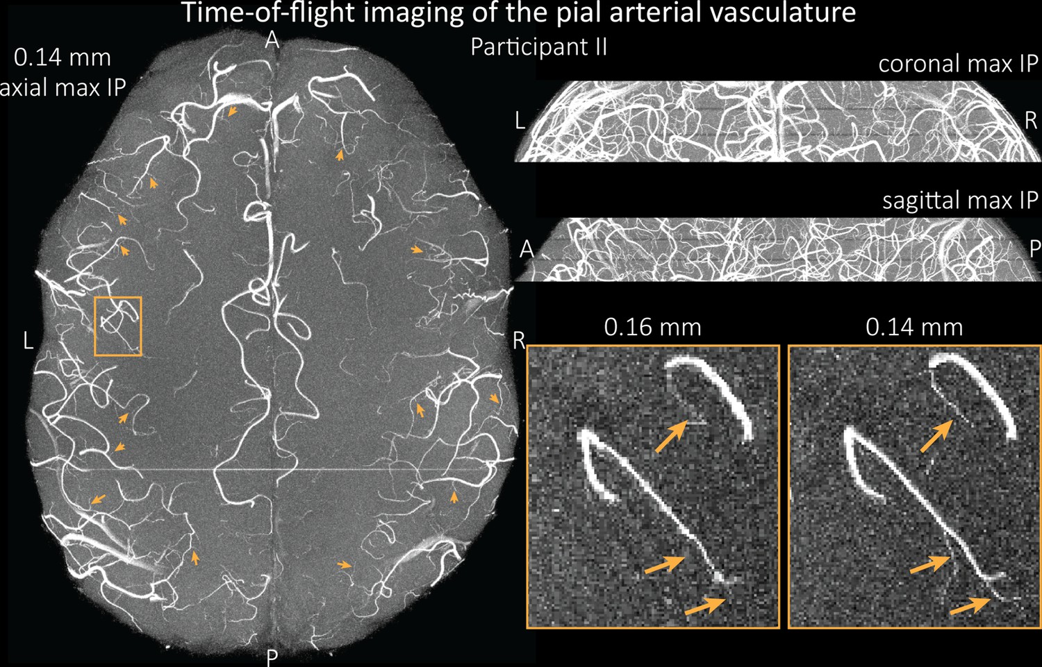
Time-of-flight imaging of the pial arterial vasculature at 0.14 mm isotropic resolution and 19.6 mm coverage in the foot-head direction showing the same data of participant II as in Figure 7, but without the overlay of the segmentation.
Left: Axial maximum intensity projection. Examples of the numerous right-angled branches are indicated by orange arrows. Right: Coronal maximum intensity projection (top) and sagittal maximum intensity projection (middle). A comparison of 0.16 and 0.14 mm voxel size (bottom) shows several vessels visible only at the higher resolution. The location of the insert is indicated on the axial maximum intensity projection on the left. Note that for this comparison, the coverage of the 0.14 mm data was matched to the smaller coverage of the 0.16 mm data.
Figure 7—figure supplement 2
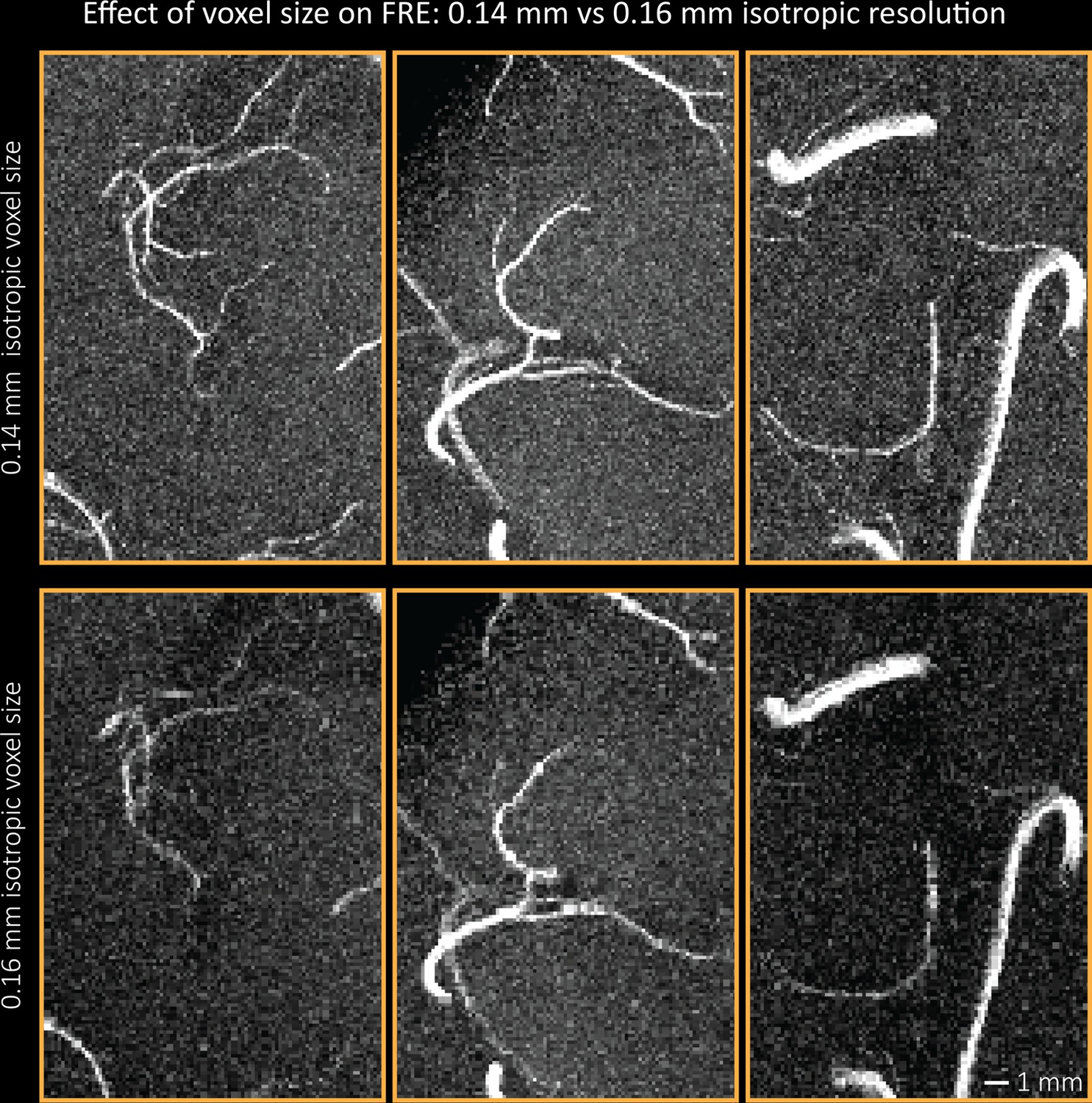
Additional examples comparing the flow-related enhancement at 0.14 mm (top) and 0.16 mm (bottom) voxel size showing additional small branches visible only at the higher resolution.
Figure 7—figure supplement 3

Small section of the time-of-flight data (13.44 mm × 9.94 mm × 7 mm) acquired at 0.14 mm isotropic resolution and the corresponding segmentation of the pial arterial vasculature from Figure 7 showing the performance of the automatic segmentation used in this study (left) and manual segmentation (right).
Figure 7—video 1
Video of the segmentation of the time-of-flight data acquired with 140 µm isotropic voxel size as shown in Figure 7.
Figure 8 with 3 supplements

Vessel displacement without correction for blood motion.
The vessel displacement is illustrated using a maximum intensity projection of the first, flow compensated echo of a two-echo time-of-flight (TOF) acquisition with the vessel centreline of the second echo without flow compensation overlaid in red. Strong displacements in both phase-encoding directions are present resulting in complex vessel shift patterns (green arrows). While furthest vessel displacements are observed in large arteries with faster flow (yellow arrows), considerable displacements arise even in smaller arteries (blue arrow).
Figure 8—figure supplement 1
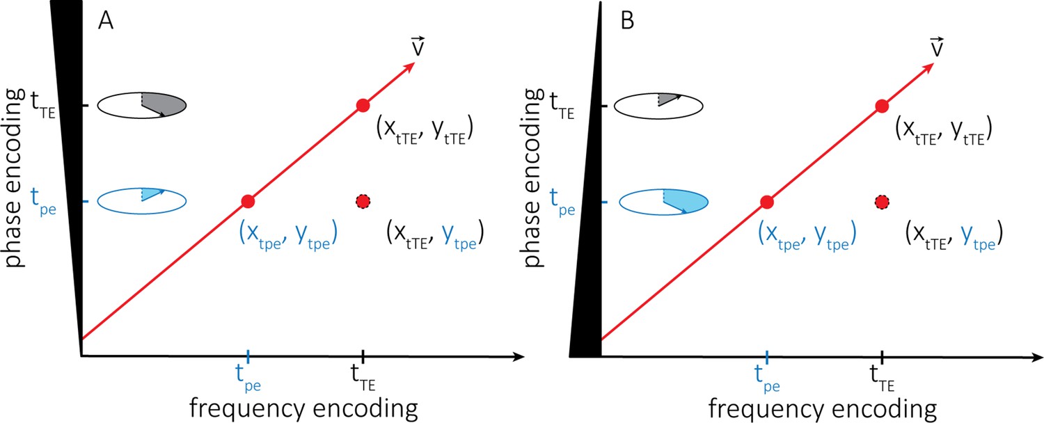
Explanation of the vessel displacement artefact.
(A) Illustration of the vessel displacement artefact in 2D caused by moving blood water spins. The blood water spins travel along the path indicated by the red arrow with velocity v and occupy different locations at the time of the phase-encoding blip (tpe) and the echo time (tTE). The resulting image location is a combination of their position at time tpe in the phase encoding direction y and their position at time tTE in the frequency encoding direction x. (B) Describes the same process but with the inverted polarity of the phase-encoding gradient.
Figure 8—video 1
Illustration of the vessel displacement artefact showing axial maximum intensity projections of the first and second echo of the two-echo time-of-flight (TOF) in Figure 8.
Figure 8—video 2
Illustration of the vessel displacement artefact showing sagittal maximum intensity projections of the first and second echo of the two-echo time-of-flight (TOF) in Figure 8.
Figure 9
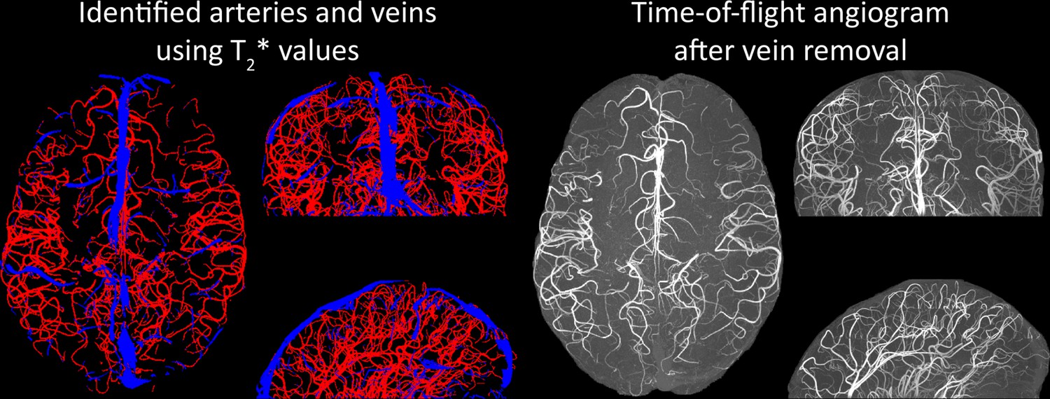
Removal of non-arterial vessels in time-of-flight imaging.
Left: Segmentation of arteries (red) and veins (blue) using estimates. Right: Time-of-flight angiogram after vein removal.
Additional files
Download links
A two-part list of links to download the article, or parts of the article, in various formats.
Downloads (link to download the article as PDF)
Open citations (links to open the citations from this article in various online reference manager services)
Cite this article (links to download the citations from this article in formats compatible with various reference manager tools)
Imaging of the pial arterial vasculature of the human brain in vivo using high-resolution 7T time-of-flight angiography
eLife 11:e71186.
https://doi.org/10.7554/eLife.71186


