3D virtual histopathology of cardiac tissue from Covid-19 patients based on phase-contrast X-ray tomography
- Institut für Röntgenphysik, Georg-August-Universität Göttingen, Friedrich-Hund-Platz, Germany
- Technical University of Denmark, Richard Petersens Plads, Denmark
- Institute of Anatomy and Cell Biology, University Medical Center of the Johannes Gutenberg-University Mainz, Germany
- Medizinische Hochschule Hannover (MHH), Germany
- Deutsches Zentrum für Lungenforschung (DZL), Hannover (BREATH), Germany
Figures
Figure 1
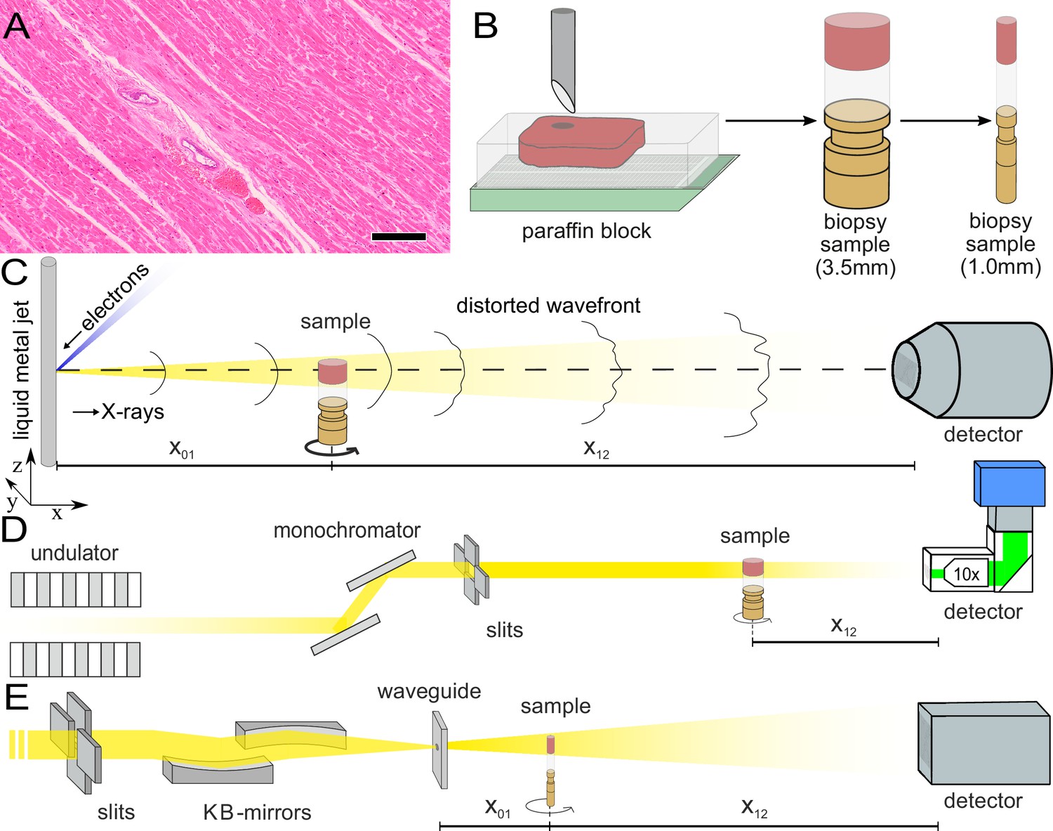
Sample preparation and tomography setups.
(A) HE stain of a 3-m-thick paraffin section of one sample from a patient who died from Covid-19 (Cov-I, Scalebar: ). In total, 26 postmortem heart tissue samples were investigated: 11 from Covid-19 patients, 4 from influenza patients, 5 from patients who died with myocarditis and six control samples. (B) From each of the samples, a biopsy punch with a diameter of was taken and transferred onto a holder for the tomography acquisition. After tomographic scans of all samples at the laboratory setup, Covid-19 and control specimens were investigated at the synchrotron. Furthermore,at the laboratory and parallel beam setup at the synchrotron, one punch with a diameter of was taken from one of the control and Covid-19 samples for investigations at high resolution. (C) Sketch of the laboratory micro-CT setup. Tomographic scans of all samples were recorded in cone beam geometry with an effective pixel size of using a liquid metal jet source (EXCILLUM, Sweden). (D) Sketch of the parallel beam setup of the GINIX endstation (P10 beamline, DESY, Hamburg). In this geometry, datasets of Covid-19 and control samples were acquired at an effective voxel size of . One plane of each sample was covered by 3×3 tomographic recordings. For each sample a plane of 3×3 tomographic acquisitions was recorded. (E) Cone beam setup of the GINIX endstation. After the investigation in parallel geometry, the 1 mm biopsy punches of one control and Covid-19 sample were probed and a high resolution scan in cone beam geometry was recorded. This configuration is based on a coherent illumination by a wave guide and allows for high geometric magnification and effective voxel sizes below .
Figure 2
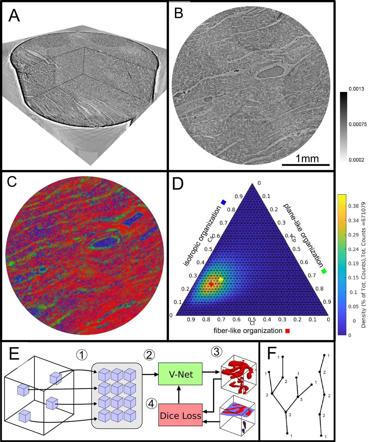
Data analysis workflow of cardiac samples.
(A) Volume rendering of a tomographic reconstruction from PB data. (B) Orthogonal slice of the masked tissue. Scale bar: (C) Shape measure distribution ( red, green and blue) of the slice shown in B. (D) Ternary plot of shape measure distribution. The peak (red) and mean (yellow) values are marked with an asterisk. (E) Overview of the training process for the neural network. (1) Random subvolumes (containing labeled voxels) are sampled from the full volume and are collected in a batch. (2) The batch is fed through the neural network, resulting in (3) a segmentation (top) and labels for one subvolume (bottom). (4) The dice loss is computed from segmented subvolumes based on labeled voxels, and the parameters of the neural network are updated. (F) Scheme of branching and the relation to degree of the vessel nodes obtained by a graph representation of the segmented microvasculature.
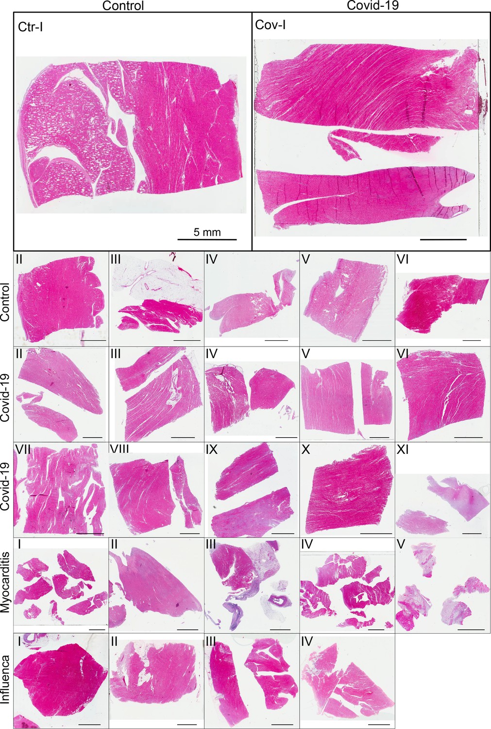
Figure 3
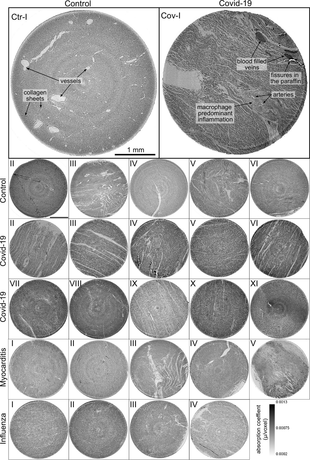
Overview of reconstruction volumes: Laboratory setup.
For each sample analyzed at the LJ µ-CT setup one slice of the reconstructed volume is shown. In the top row, a slice of a tomographic reconstruction of a control sample (Ctr-I) and of a sample from a patient who died from Covid-19 (Cov-I) are shown. Below, further slices from control (Ctr-II to Ctr-VI), Covid-19 (Cov-II to Cov-XI) as well as myocarditis (Myo-I to Myo-V) and influenza (Inf-I to Inf-IV) samples are shown. Scale bars: .
Figure 4
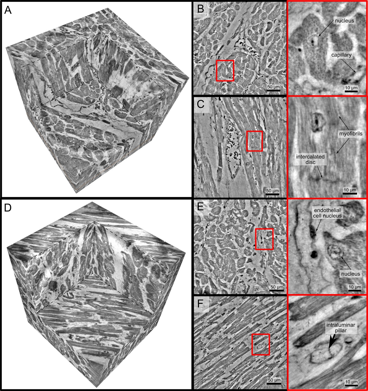
High-resolution tomogram of cardiac tissue recorded in cone beam geometry.
(A) Volume rendering of a tomographic reconstruction from a control sample recorded in cone beam geometry based on a wave guide illumination. After the analysis in parallel beam geometry, a biopsy with a diameter of was taken from the biopsy punch. This configuration revealed sub-cellular structures such as nuclei of one cardiomyocytes, myofibrils and intercalated discs. (B) Slice of the reconstructed volume perpendicular to the orientation of the cardiomyocytes. The red box marks an area which is magnified and shown on the right. One cardiomyocyte is located in the center of the magnified area. In this view, the nucleus can be identified. It contains two nucleoli, which can be identified as dark spots. The myofibrils appear as round discs. (C) Orthogonal slice which oriented along the orientation of the cardiomyocytes. A magnification of the area marked with a red box. In this view, a nucleus but also the myofibrils can be identified as dark, elongated structures in the cell. Further, an intercalated disc is located at the bottom of the area. (D) Volume rendering of a tomographic reconstruction from a Covid-19 sample. Slices orthogonal (E) and along (F) to the cardiomyocyte orientation are shown on the right. In the magnified areas, a nucleus of an endothelial cell and an intraluminar pillar -the morphological hallmark of intussusceptive angiogenesis- are visible. Scale bars: orthoslices ; magnified areas .
Figure 5

Clustering of LJ data sets.
(A) Ternary diagram of the mean value of the shape measures for all datasets. The control samples (green) show low values, while samples from Covid-19 (red), influenza and myocarditis (blue) patients show a larger variance for . (B) The fitted area of the elliptical fit from the PCA analysis of the shape measure distribution is an indicator for the variance in tissue structure. For Control and influenza sample this value differs significantly from the Covid-19 tissue. (C) The eccentricity of the fit indicates if the structural distribution in shape measure space has a preferred direction along any axis. The value of the myocarditis samples is comparable low.
Figure 6
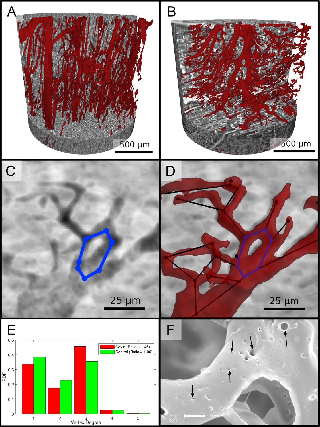
Segmentation of the vascular system in cardiac samples.
(A) Segmentation of the vessels of a Ctr sample. The vessels are well oriented and show a relatively constant diameter. (B) Segmentation of the vessels of a Covid-19 sample. The vessels show large deviations in diameter and the surface of the vessels is not as smooth as in the control sample. (C) Filtered minimum projection of an area of the reconstructed electron density of the Cov sample to highlight a vessel loop marked in blue. (D) Surface rendering of the segmented vessel and vessel graph in an area of the Cov sample. Scale bars . (E) Comparison of node degree between control and Covid-19. Ratio refers to the number of graph branch points ( > 2) divided by the number of end points ( = 1). (F) Exemplary scanning electron microscopy image of a microvascular corrosion casting from a Covid-19 sample. The black arrows mark the occurrence of some tiny holes indicating intraluminar pillars with a diameter of to , indicating intussusceptive angiogenesis. Magnification x800, scale bar .
Appendix 1—figure 1
HE stain of all cardiac samples .
Scale bar: .
Appendix 1—figure 2
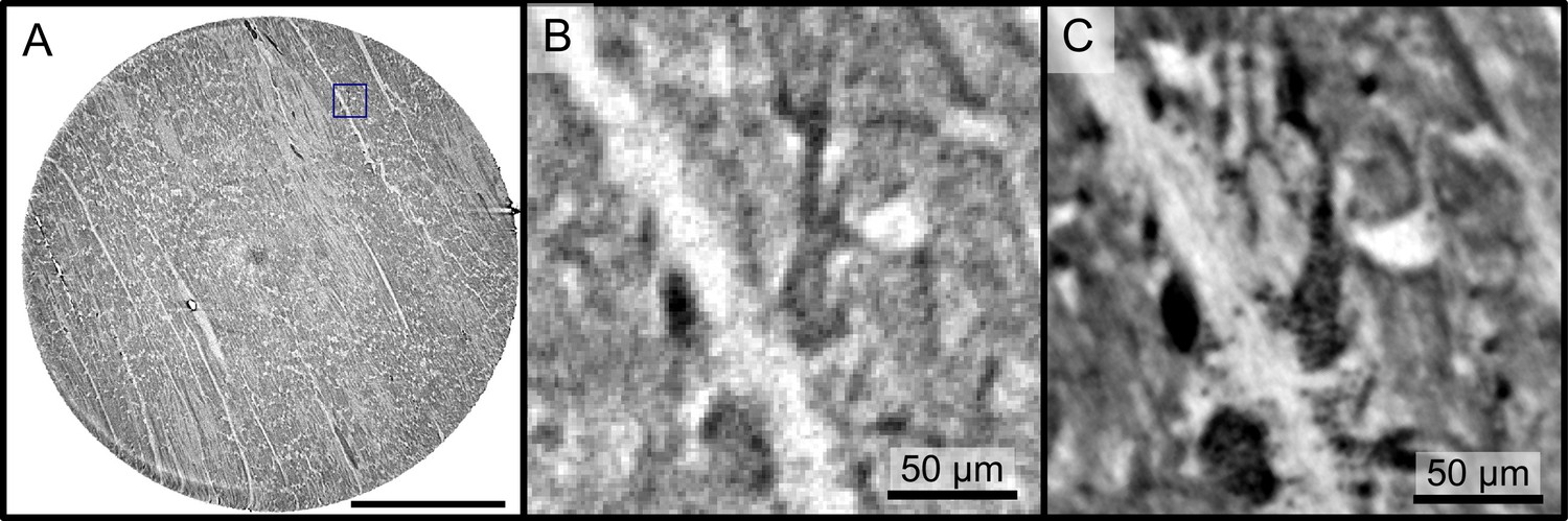
Reconstructions of the LJ compared to the PB setup.
Comparison of the data quality of laboratory and synchrotron measurements. (A) slice of a laboratory reconstruction at a voxelsize of . A region of interest containing a branching vessel is marked by a blue box which is shown in (B). The same area cropped from a tomographic reconstruction at the PB setup at a voxelsize of is shown in (C). The smaller voxelsize, higher contrast and SNR of the PB scans is necessary to segment the vascular system. Scale bars: (A) , (B,C).
Appendix 1—figure 3

Shape measure of all Covid-19 and control samples reconstructed from PB data.
Slices of the reconstructed electron density (stitched volumes of 3 ×three tomographic reconstructions), the corresponding slice of the shape measure and the ternary plot of the shape distribution in the entire volume are shown. Corrupted datasets were excluded from the analysis and masked in white. Scale bar: .
Tables
Table 1
Sample and medical information of patients.
| Sample group | N patients | Sample quantity | Age | Sex |
|---|---|---|---|---|
| Control | 2 | 6 | 31 ± 7 | 2 F |
| Covid-19 | 11 | 11 | 76 ± 13 | 10 M, 1 F |
| Myocarditis | 5 | 5 | 43 ± 17 | 4 M, 1 F |
| Influenza | 4 | 4 | 63 ± 9 | 3 M, 1 F |
Table 2
Data acquisition parameters of the laboratory and synchrotron scans.
| Parameter | LJ setup | PB setup | WG setup (Ctr/Cov) |
|---|---|---|---|
| Photon energy (keV) | 9.25 | 13.8 | 10/10.8 |
| Source-sample-dist. x01 (m) | 0.092 | 0.125/0.125 0.127 0.131 0.139 | |
| Sample-detector-dist. x12 (m) | 0.206 | 0.5 | 4.975 |
| Geometric magnification M | |||
| Pixel size (µm) | 6.5 | 0.65 | 6.5 |
| Effective pixel size (µm) | 2 | 0.65 | 0.159 |
| Field-of-view h×v (mm2) | 4.8×3.4 | 1.6× 1.4 | 0.344×0.407/0.325× 0.325 |
| Acquisition time (s) | 3× 0.6 | 0.035 | 0.3/2.5 |
| Number of projections | 1501 | 3000 | 1500 |
| Number of flat fieldempties | 50 | 1000 | 50 |
| Number of dark field | 50 | 150 | 20 |
Table 3
Phase retrieval algorithms and parameters used for the different setups.
| Setup | LJ setup | PB setup configuration | WG setup configuration |
|---|---|---|---|
| Fresnel number | 0.47125 | 0.0095 | 0.0017 |
| phase retrieval | BAC | CTF | nonlinear CTF |
| -ratio | - | 1/45 | 1/130 |
| parameter | = | = | = |
| = 1 | = 0.5 | = 0.2 |
Table 4
Parameters of the cardiac tissue obtained from LJ reconstructions.
For all sample groups the mean value and standard deviation of the mean shape measures , , area of the elliptical fit (%) and the eccentricity is shown.
| Group | (%) | ||||
|---|---|---|---|---|---|
| Control | 0.60± 0.11 | 0.18± 0.07 | 0.22± 0.06 | 11.98± 6.42 | 0.61± 0.13 |
| Covid-19 | 0.44±0.12 | 0.23±0.03 | 0.32±0.11 | 16.92± 2.91 | 0.61± 0.09 |
| Myocarditis | 0.47±0.14 | 0.21± 0.02 | 0.33±0.13 | 16.69± 5.06 | 0.51± 0.12 |
| Influenza | 0.49±0.11 | 0.16±0.02 | 0.35±0.12 | 13.44± 1.31 | 0.63± 0.07 |
Appendix 2—table 1
Sample and medical information.
Age and sex, clinical presentation with hospitalization and treatment. RF:respiratory failure, CRF: cardiorespiratory failure, MOF: multi-organ failure, V: ventilation, S: Smoker, D: Diabetes TypeII, H: Hypertension, I: imunsupression
| Sample no. | Age, sex | Hospitalization (days), clinical, radiological and histological characteristics |
|---|---|---|
| Cov-I | 86,M | 5d, RF, D, H, I |
| Cov-II | 96,M | 3d, RF, H |
| Cov-III | 78,M | 3d, CRF, V, D, S, H |
| Cov-IV | 66,M | 9d, RF, V, S, H |
| Cov-V | 74,M | 3d, RF, D, S, H |
| Cov-VI | 81,F | 4d, RF, S, H |
| Cov-VII | 71,M | 0d, V |
| Cov-VIII | 88,M | 2d, V, H, I |
| Cov-IX | 85,M | 5d, V, S, H |
| Cov-X | 58,M | 7d, V, H |
| Cov-XI | 54,M | 15d, V |
| Ctr-I to Ctr-III | 26, F | - |
| Ctr-IV to Ctr-VI | 36, F | - |
| Myo-I | 57,M | V, H |
| Myo-II | 23,M | |
| Myo-III | 59,M | S, H, D |
| Myo-IV | 50,M | V, S, D |
| Myo-V | 25,F | |
| Inf-I | 74,M | 9d, CRF into MOF, V, S, H |
| Inf-II | 66,F | 17d, MOF, V, H |
| Inf-III | 56,M | 3d, CRF into MOF, V |
| Inf-IV | 55,M | 24d, RF into MOF, V, S |
Appendix 2—table 2
Parameters of the cardiac tissue (laboratory data).
| Sample | Mean (Cl,Cp, Cs) | Fitted area | Eccentricity |
|---|---|---|---|
| Ctr-I | (0.6508, 0.1069, 0.2423 ) | 7.3194 | 0.5607 |
| Ctr-II | ( 0.5167, 0.1907, 0.2926 ) | 11.5130 | 0.5736 |
| Ctr-III | ( 0.5074, 0.2427, 0.2499) | 23.7443 | 0.4128 |
| Ctr-IV | ( 0.7434, 0.1166, 0.1400 ) | 5.9026 | 0.6757 |
| Ctr-V | ( 0.7038, 0.1495, 0.1467 ) | 9.5763 | 0.7896 |
| Ctr-VI | ( 0.4765, 0.2835, 0.2400 ) | 13.7973 | 0.6688 |
| mean | (0.60 ± 0.11. 0.18 ± 0.07, 0.22 ± 0.06) | 11.98 ± 6.42 | 0.61 ± 0.13 |
| Cov-I | ( 0.5398, 0.2327, 0.2275) | 12.7052 | 0.6696 |
| Cov-II | ( 0.4676, 0.2550, 0.2774 ) | 17.0347 | 0.6059 |
| Cov-III | ( 0.5896, 0.2526, 0.1578) | 11.8845 | 0.7399 |
| Cov-IV | ( 0.5911, 0.1833, 0.2255 ) | 16.3040 | 0.6765 |
| Cov-V | ( 0.3371, 0.2505, 0.4124) | 16.3445 | 0.4081 |
| Cov-VI | ( 0.5184, 0.2279, 0.2537) | 19.1954 | 0.6044 |
| Cov-VII | (0.3912, 0.2262, 0.3826) | 19.8206 | 0.6530 |
| Cov-VIII | ( 0.5227, 0.1776, 0.2997) | 15.0791 | 0.6033 |
| Cov-IV | (0.3253, 0.2851, 0.3897 ) | 20.5768 | 0.5329 |
| Cov-X | (0.3283, 0.2446, 0.4271 ) | 16.9989 | 0.6266 |
| Cov-XI | ( 0.2484, 0.2314, 0.5202 ) | 20.1815 | 0.5407 |
| mean | ( ) | 16.92 ± 2.91 | 0.61 ± 0.09 |
| Myo-I | (0.5777, 0.2018, 0.2206 ) | 9.5528 | 0.4656 |
| Myo-II | (0.3887, 0.1943, 0.4170 ) | 13.7853 | 0.4899 |
| Myo-III | ( 0.5984, 0.2081, 0.1935 ) | 22.4768 | 0.6202 |
| Myo-IV | ( 0.4974, 0.1908, 0.3117 ) | 18.3306? | 0.6149 |
| Myo-V | (0.2664, 0.2402, 0.4933 ) | 19.3212 | 0.3689 |
| mean | (0.27 ± 0.14, 0.24 ± 0.02, 0.49 ± 0.13) | 16.69 ± 5.06 | 0.51 ± 0.12 |
| Inf-I | (0.3561, 0.1714, 0.4724 ) | 14.9393 | 0.6808 |
| Inf-II | ( 0.4423, 0.1376, 0.4201 ) | 11.7445? | 0.5991 |
| Inf-III | ( 0.6150, 0.1361, 0.2489 ) | 13.5988 | 0.7198 |
| Inf-IV | ( 0.5404, 0.1849, 0.2747 ) | 13.4885 | 0.5561 |
| mean | (0.49 ± 0.11, 0.16 ± 0.02, 0.35 ± 0.11) | 13.44 ± 1.31 | 0.63 ± 0.07 |
Additional files
Download links
A two-part list of links to download the article, or parts of the article, in various formats.
Downloads (link to download the article as PDF)
Open citations (links to open the citations from this article in various online reference manager services)
Cite this article (links to download the citations from this article in formats compatible with various reference manager tools)
3D virtual histopathology of cardiac tissue from Covid-19 patients based on phase-contrast X-ray tomography
eLife 10:e71359.
https://doi.org/10.7554/eLife.71359


