Humans actively sample evidence to support prior beliefs
- Department of Experimental Psychology, University of Oxford, United Kingdom
- Wellcome Centre for Integrative Neuroimaging, University of Oxford, United Kingdom
- Institute of Cognitive Neuroscience, University College London, United Kingdom
- Department of Mathematics and Computer Science, Rutgers University, United States
- Centre for Business Research, Cambridge Judge Business School, University of Cambridge, United Kingdom
- Department of Economics and Woodrow Wilson School, Princeton University, United States
- Wellcome Centre for Human Neuroimaging, University College London, United Kingdom
Figures
Figure 1
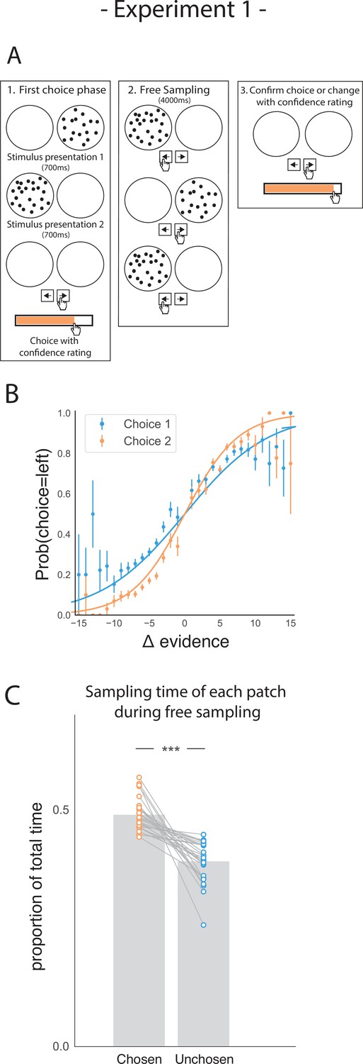
Task design and participant behaviour for experiment 1.
(A) Task structure. Participants had to choose which of two dot patches contained the most dots after viewing each for 700ms (phase 1) and rate their confidence in this choice. Then participants were given 4000ms to view the dots which they could allocate between the two patches in whichever way they liked (phase 2) by pressing the left and right arrow keys. Finally, participants made a second choice about the same set of stimuli and rated their confidence again (phase 3). (B) Participants effectively used the stimuli to make correct choices and improved upon their performance on the second choice. This psychometric curve is plotting the probability of choosing the left option as a function of the evidence difference between the two stimuli for each of the two choice phases. (C) In the free sampling phase (phase 2) participants spent more time viewing the stimulus they chose on the preceding choice phase than the unchosen option. Data points represent individual participants.
Figure 2 with 1 supplement
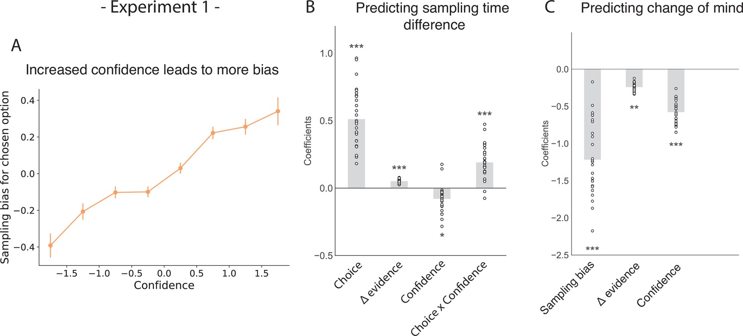
The effect of choice on sampling behavior is mediated by confidence in experiment 1.
Participants were less likely to change their mind if they showed a strong sampling bias for their initially chosen option in the sampling phase. (A) Sampling bias in favour of the chosen option increases as a function of confidence in the initial choice. Confidence and sampling bias are both normalised at the participant level in this plot. (B) There is a significant main effect of choice on sampling time difference, such that an option is sampled for longer if it was chosen, and a significant interaction effect of Choice x Confidence, such that options chosen with high confidence are sampled for even longer. (C) There is a main negative effect of sampling bias on change of mind, such that participants were less likely to change their mind in the second decision phase (phase 3) the more they sampled their initially chosen option in the free sampling phase (phase 2). (B–C) Plotted are fixed-effect coefficients from hierarchical regression models predicting the sampling time (how long each patch was viewed in the sampling phase) difference between the left and right stimuli. Data points represent regression coefficients for each individual participant.
Figure 2—figure supplement 1
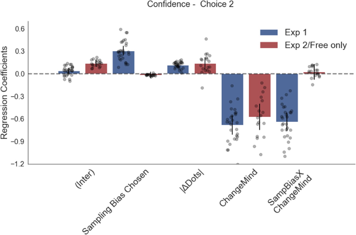
Confidence in the second choice is significantly predicted by trial difficulty (dot difference) and change of mind.
In experiment 1, it is also affected by sampling bias, such that the more time participants spent sampling the initially chosen stimulus, the more confidence they had in their second choice. Plotted are fixed-effect coefficients from hierarchical regression models predicting confidence ratings in the second choice phase. Data points represent regression coefficients for each individual participant.
Figure 3 with 1 supplement
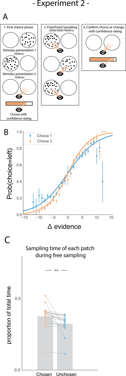
Task design and participant behaviour for experiment 2.
(A) Task structure. Participants had to choose which of two dot patches contained the most dots after viewing each for 500ms (phase 1) and rate their confidence in this choice. Then participants were given 3000ms, 5000ms, or 7000ms to view the dots which they could allocate between the two patches in whichever way they liked (phase 2) by looking inside the circles. Finally, participants made a second choice about the same set of stimuli and rated their confidence again (phase 3). (B) Participants effectively used the stimuli to make correct choices and improved upon their performance on the second choice. This psychometric curve is plotting the probability of choosing the left option as a function of the evidence difference between the two stimuli for each of the two choice phases. (C) In the free sampling condition during the sampling phase (phase 2) participants spent more time viewing the stimulus they chose on the preceding choice phase than the unchosen option. Data points represent individual participants.
Figure 3—figure supplement 1
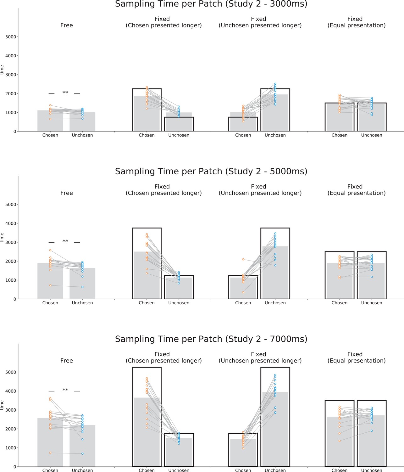
Mean sampling time viewing the initially chosen and unchosen patch in the sampling phase in study 2 for each sampling phase length and each condition.
For the fixed condition, trials have been split into trials where the stimulus chosen in the first choice phase was shown for longer (‘chosen presented longer’), trials where the unchosen was shown for longer (‘unchosen presented longer’) and trials where both stimuli were shown for equal amounts of time (‘equal presentation’). The black rectangles show the amount of time each stimulus was presented on those trials. Data points represent individual participants.
Figure 4 with 12 supplements
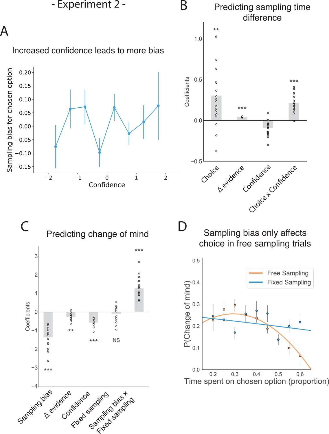
The effect of choice on sampling behaviour is mediated by confidence in experiment 2.
Participants were less likely to change their mind if they showed a strong sampling bias for their initially chosen option in the sampling phase, but this was only the case in the free sampling condition. (A) Sampling bias in favour of the chosen option increases as a function of confidence in the initial choice. Confidence and sampling bias towards the chosen option are both normalized at the participant level in this plot. (B) There is a significant main effect of choice on sampling time difference, such that an option is sampled for longer if it was chosen, and a significant interaction effect of Choice x Confidence, such that options chosen with high confidence are sampled for even longer. (C) There is a main negative effect of sampling bias on change of mind, such that participants were less likely to change their mind in the second decision phase (phase 3) the more they sampled their initially chosen option in the free sampling phase (phase 2). The main effect of sampling bias on change of mind disappears in the fixed sampling condition, which can be seen by the positive interaction term Sampling bias x Fixed sampling which entirely offsets the main effect. The analysis includes a dummy variable ‘Fixed Sampling’ coding whether the trial was in the fixed-viewing condition. (B–C) Plotted are fixed-effect coefficients from hierarchical regression models predicting the sampling time (how long each patch was viewed in the sampling phase) difference between the left and right stimuli. Data points represent regression coefficients for each individual participant. (D) The probability that participants change their mind on the second choice phase is more likely if they looked more at the unchosen option during the sampling phase. The plot shows the probability that participants changed their mind as a function of the time spent sampling the initially chosen option during phase 2. The lines are polynomial fits to the data, while the data points indicate the frequency of changes of mind binned by sampling bias. Note that actual gaze time of the participants is plotted here for both task conditions. The same pattern can be seen when instead plotting the fixed presentation times of the stimuli for the fixed task condition (see Figure 4—figure supplement 2).
Figure 4—figure supplement 1
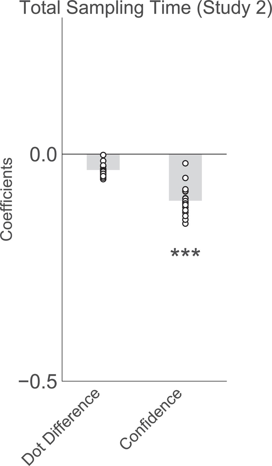
Confidence in the first choice reduces the total amount of time spent sampling (gazing at the two stimuli) in the free sampling trials in experiment 2.
Plotted are fixed-effect coefficients from a hierarchical regression model predicting total sampling time (the total time spent gazing at the stimuli). Data points represent regression coefficients for each individual participant.
Figure 4—figure supplement 2
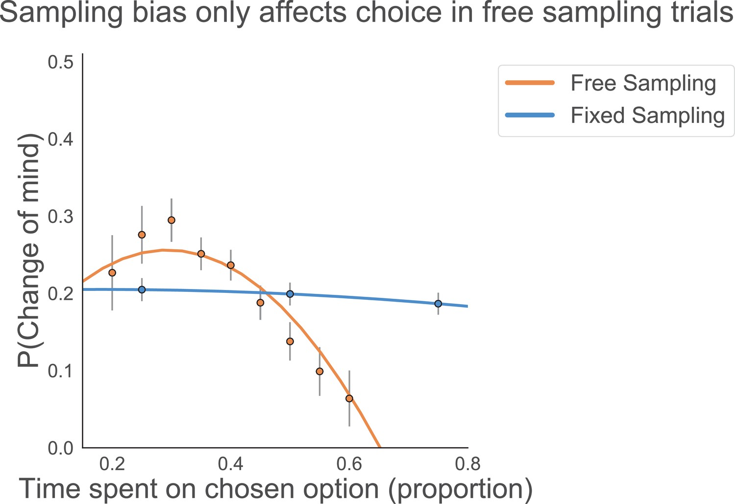
In Figure 4D, we plotted the probability of changes of mind as a function of actual gaze time by participants in the fixed viewing condition.
Even though stimulus presentation was fixed, participants could still choose to saccade back to the central fixation cross before the end of stimulus presentation. Therefore, actual gaze time is a better reflection of information processing in this condition. Here, we are plotting stimulus presentation time in the fixed sampling condition instead. The same lack of effect of sampling bias on changes of mind can be seen here in the fixed sampling condition as in Figure 4.
Figure 4—figure supplement 3
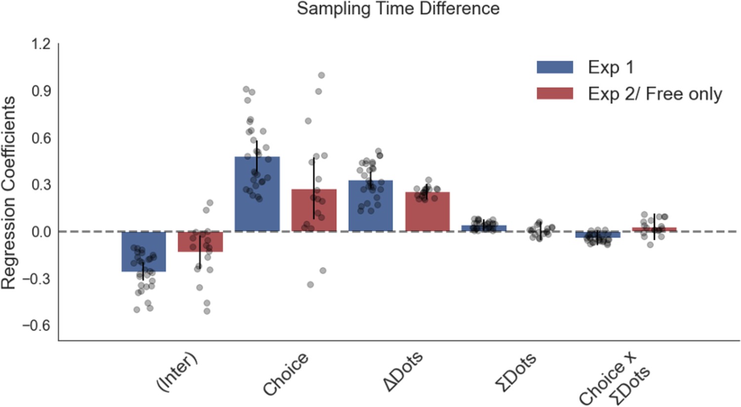
Numerosity has no significant effect on sampling bias in a regression analysis predicting sampling bias with total numerosity (total number of dots present on a trial) included as a predictor.
Plotted are fixed-effect coefficients from hierarchical regression models predicting the sampling time (how long each patch was viewed in the sampling phase) difference between the left and right stimuli. Data points represent regression coefficients for each individual participant.
Figure 4—figure supplement 4
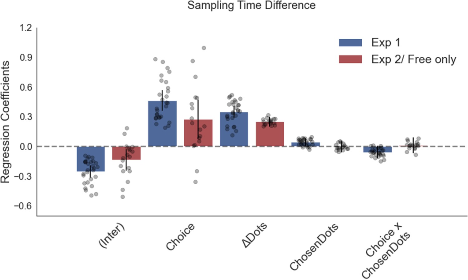
Numerosity has no significant effect on sampling bias in a regression analysis predicting sampling bias with numerosity of the chosen stimulus (dots in the chosen stimulus) included as a predictor.
Plotted are fixed-effect coefficients from hierarchical regression models predicting the sampling time (how long each patch was viewed in the sampling phase) difference between the left and right stimuli. Data points represent regression coefficients for each individual participant.
Figure 4—figure supplement 5
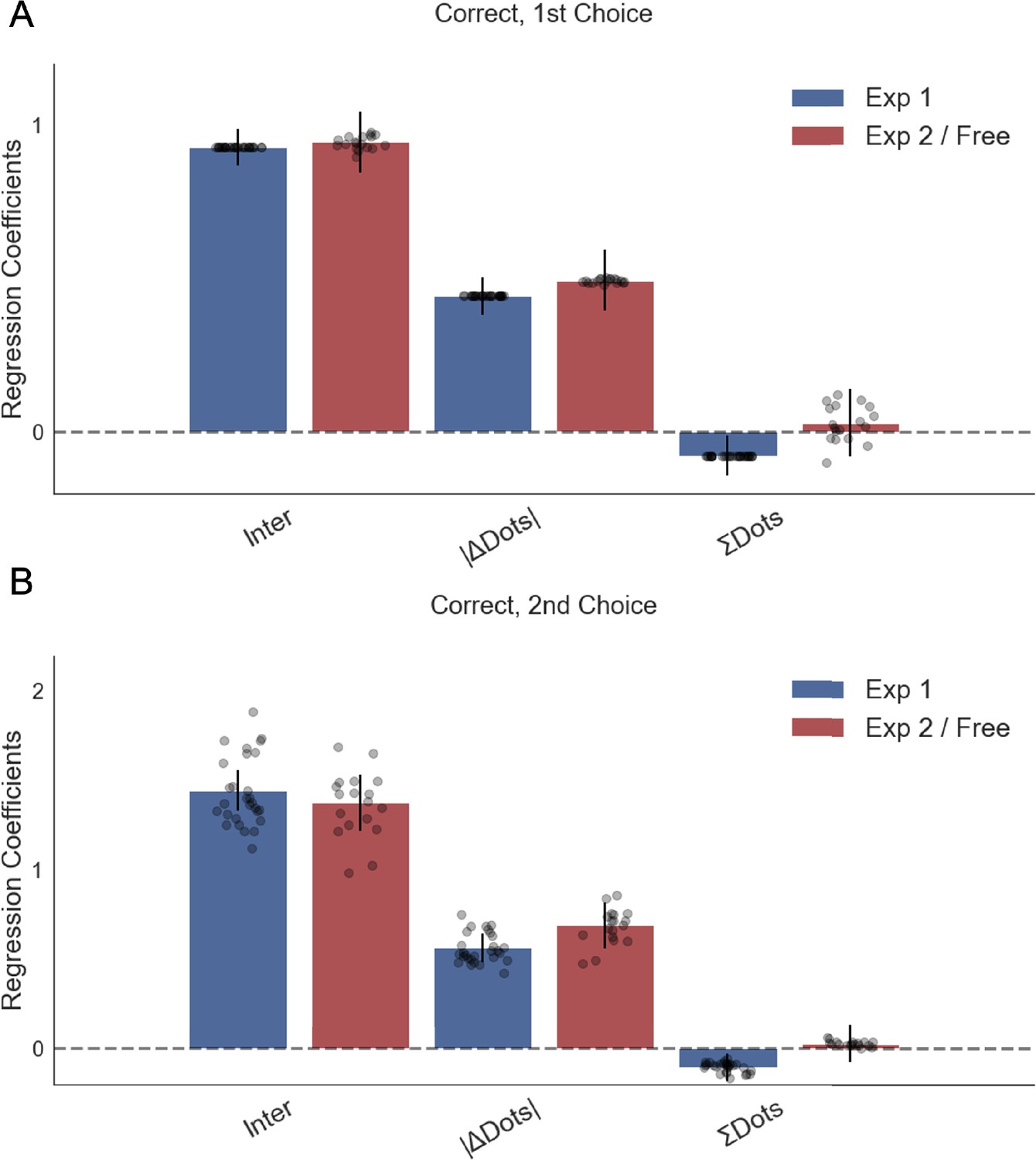
Numerosity had a small significant effect on accuracy in the first choice phase in experiment 1, such that participants made more mistakes on trials with high total numerosity (total number of dots).
This effect was not significant for the second choice phase and for neither choice phase in experiment 2. Plotted are fixed-effect coefficients from hierarchical logistic regression models predicting the trial accuracy in the first and second choice phases. Data points represent regression coefficients for each individual participant.
Figure 4—figure supplement 6
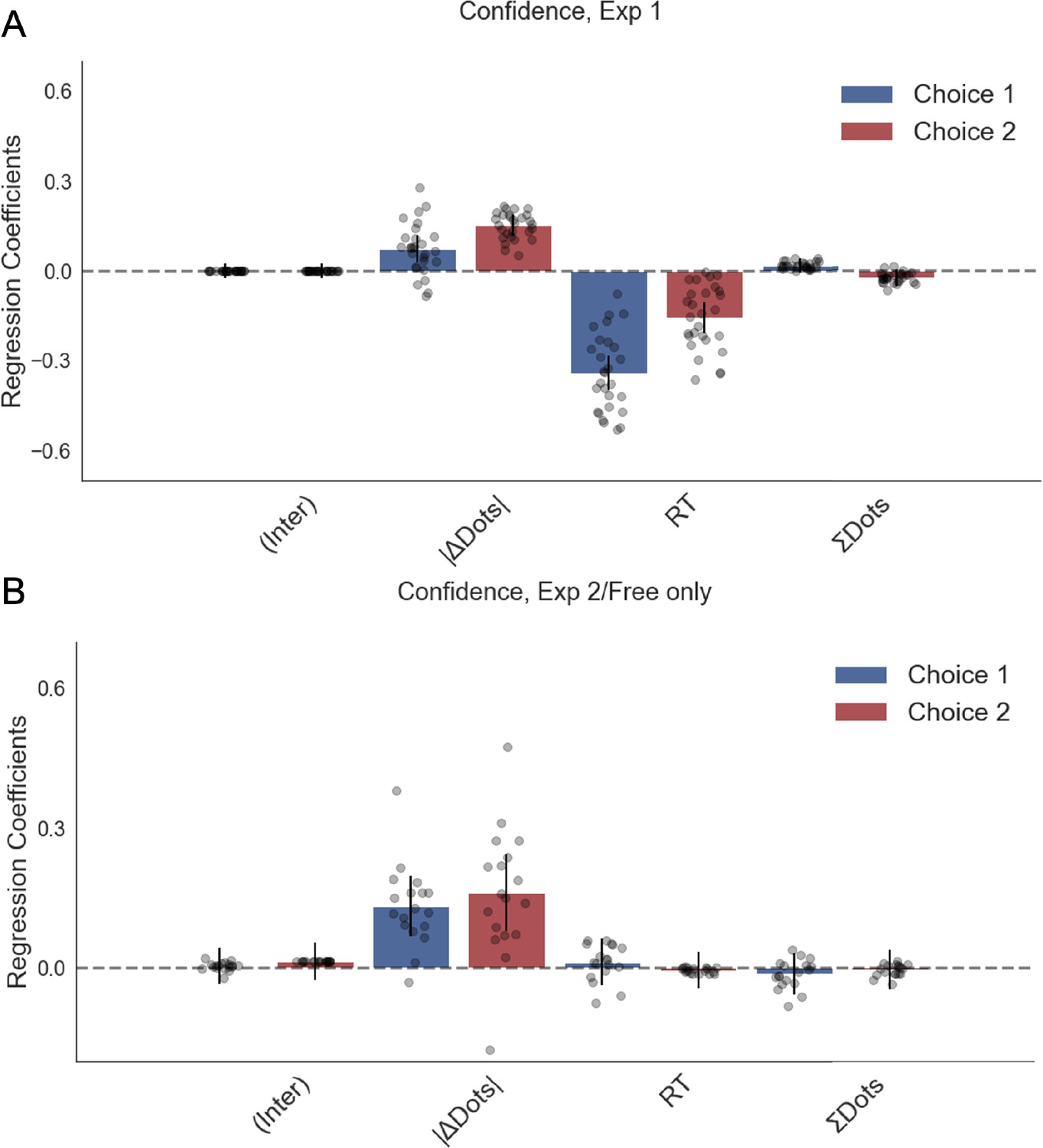
Confidence was not affected by numerosity in a linear regression model.
Plotted are fixed-effect coefficients from hierarchical regression models predicting confidence ratings on the first and second choice phases. Data points represent regression coefficients for each individual participant.
Figure 4—figure supplement 7
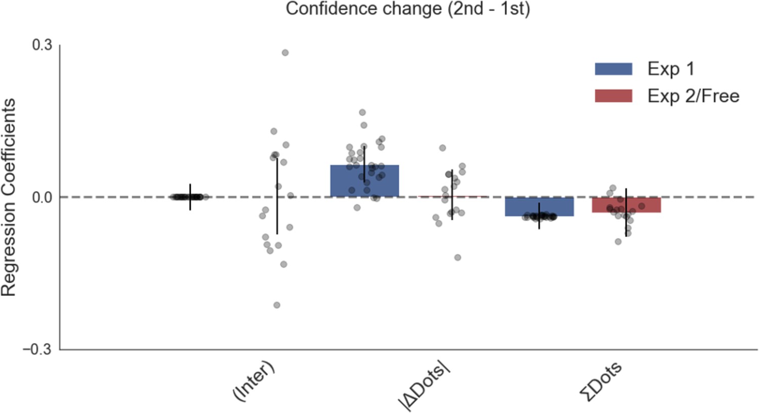
Confidence change in experiment 1 was negatively affected by total numerosity (total number of dots), although it is a small effect.
This means confidence from the first to the second choice phase changed less on trials with higher total numerosity. Plotted are fixed-effect coefficients from hierarchical regression models predicting confidence change between the first and second choice phases. Data points represent regression coefficients for each individual participant.
Figure 4—figure supplement 8
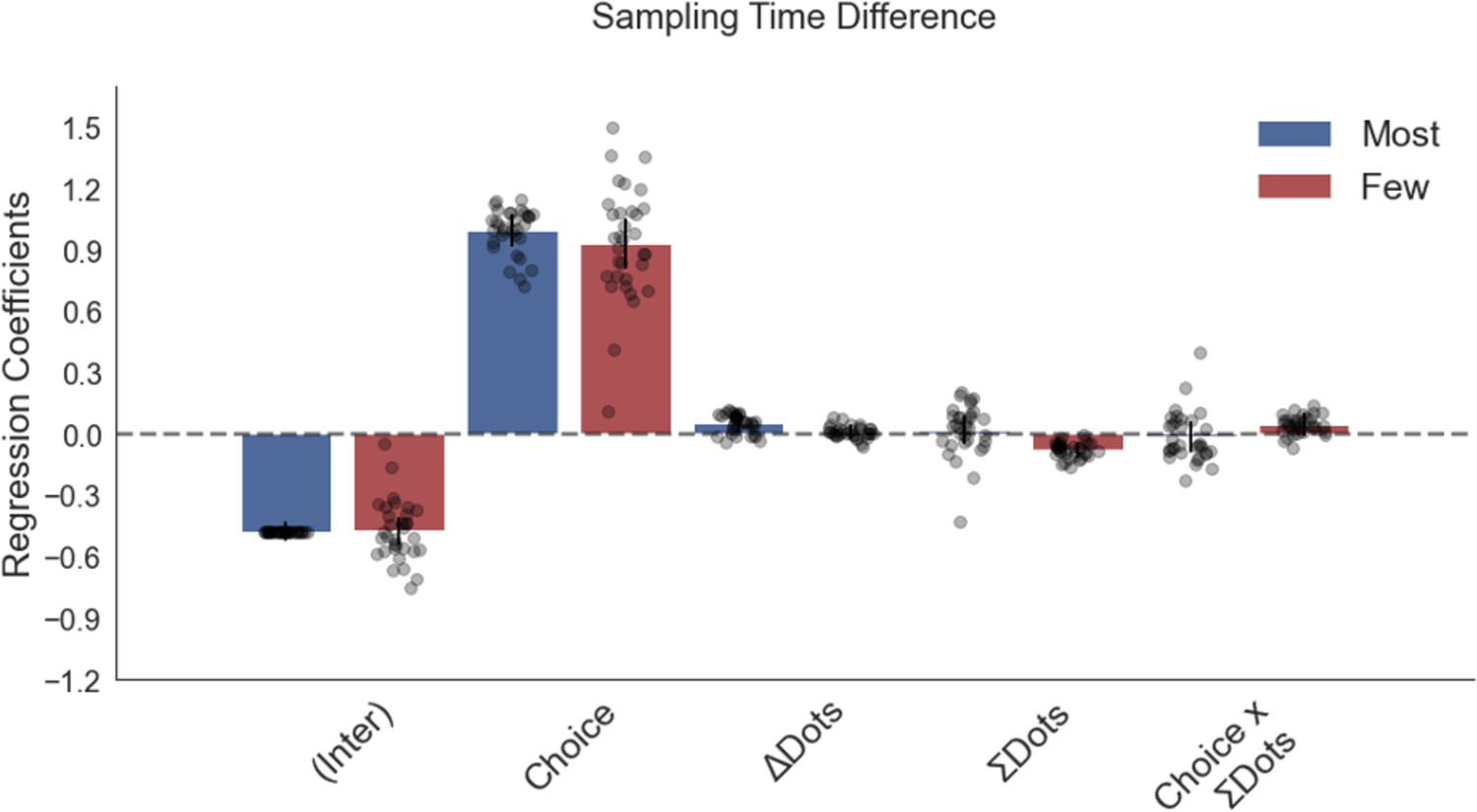
A sampling bias towards the stimulus that participants would end up choosing was found in an independent dataset from a perceptual experiment presented in Sepulveda et al., 2020, and this was not affected by total numerosity ()on a trial.
In this experiment, participants performed a dot numerosity task in two frames: in the ‘most’ frame they chose the alternative with more dots, in the ‘fewest’ frame they indicated the option with fewer dots. Plotted are fixed-effect coefficients from hierarchical regression models predicting the sampling time (how long each patch was viewed in the initial sampling phase before choosing) difference between the left and right stimuli. Data points represent regression coefficients for each individual participant.
Figure 4—figure supplement 9
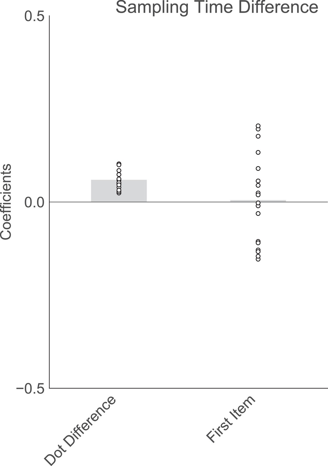
Order of presentation has no significant effect on sampling bias in experiment 2.
Plotted are fixed-effect coefficients from a hierarchical regression model predicting the sampling time (how long each patch was viewed in the sampling phase) difference between the left and right stimuli. Data points represent regression coefficients for each individual participant.
Figure 4—figure supplement 10
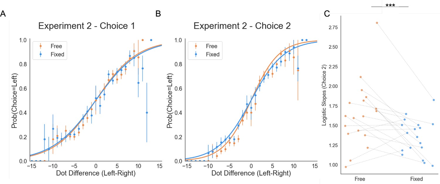
Choice behaviour in Experiment 2.
(A) Initial choice (pre-sampling) (B) Final choice (post-sampling). (C) Participants were more precise in selecting the circle with more dots in the Free sampling trials, as seen from participants’ higher slopes of the logistic curve.
Figure 4—figure supplement 11
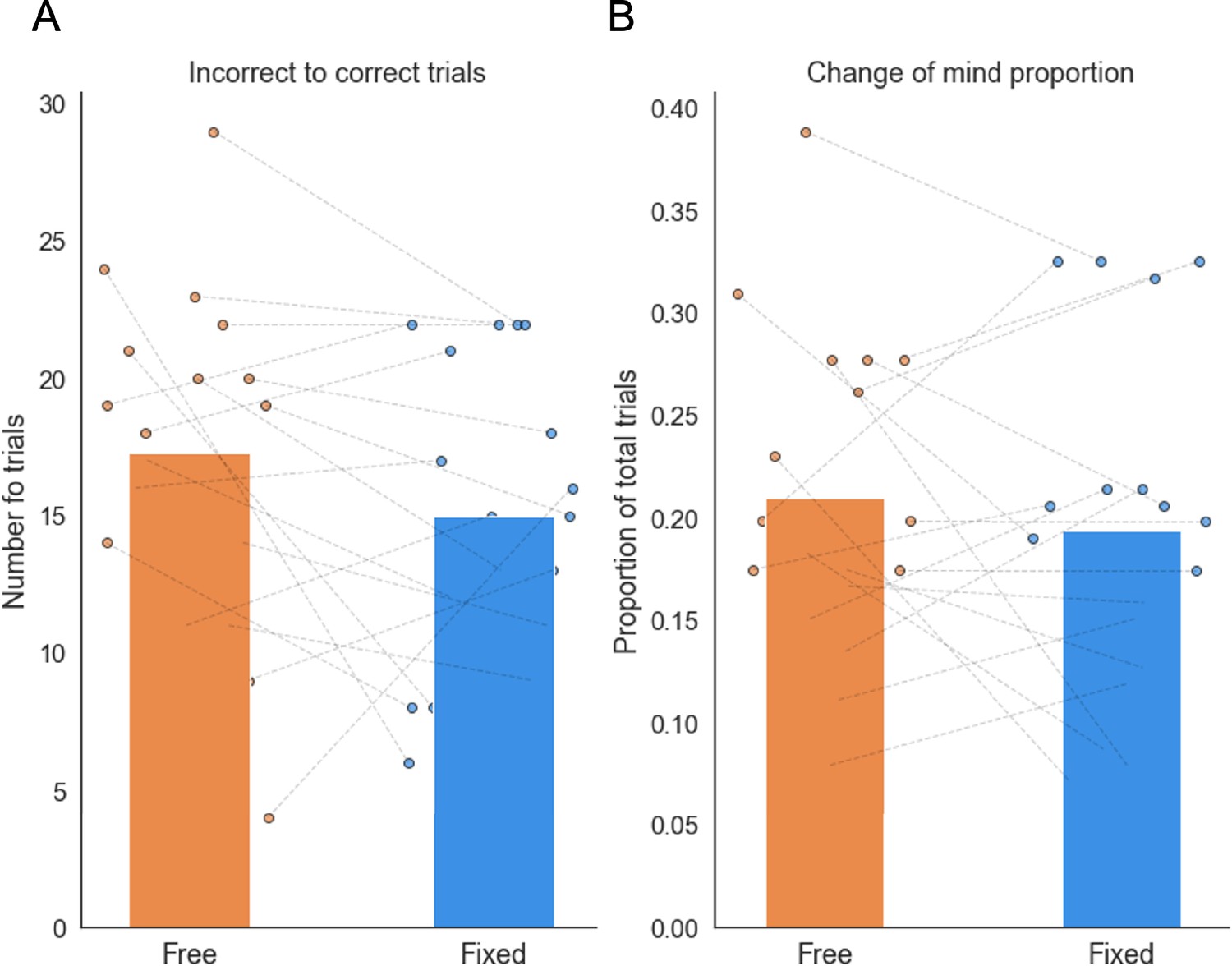
There was no significant difference in the number of changes of mind from the incorrect to the correct option (A) or in the total number of changes of mind (B) between the free and fixed sampling conditions.
Data points represent individual participants.
Figure 4—figure supplement 12
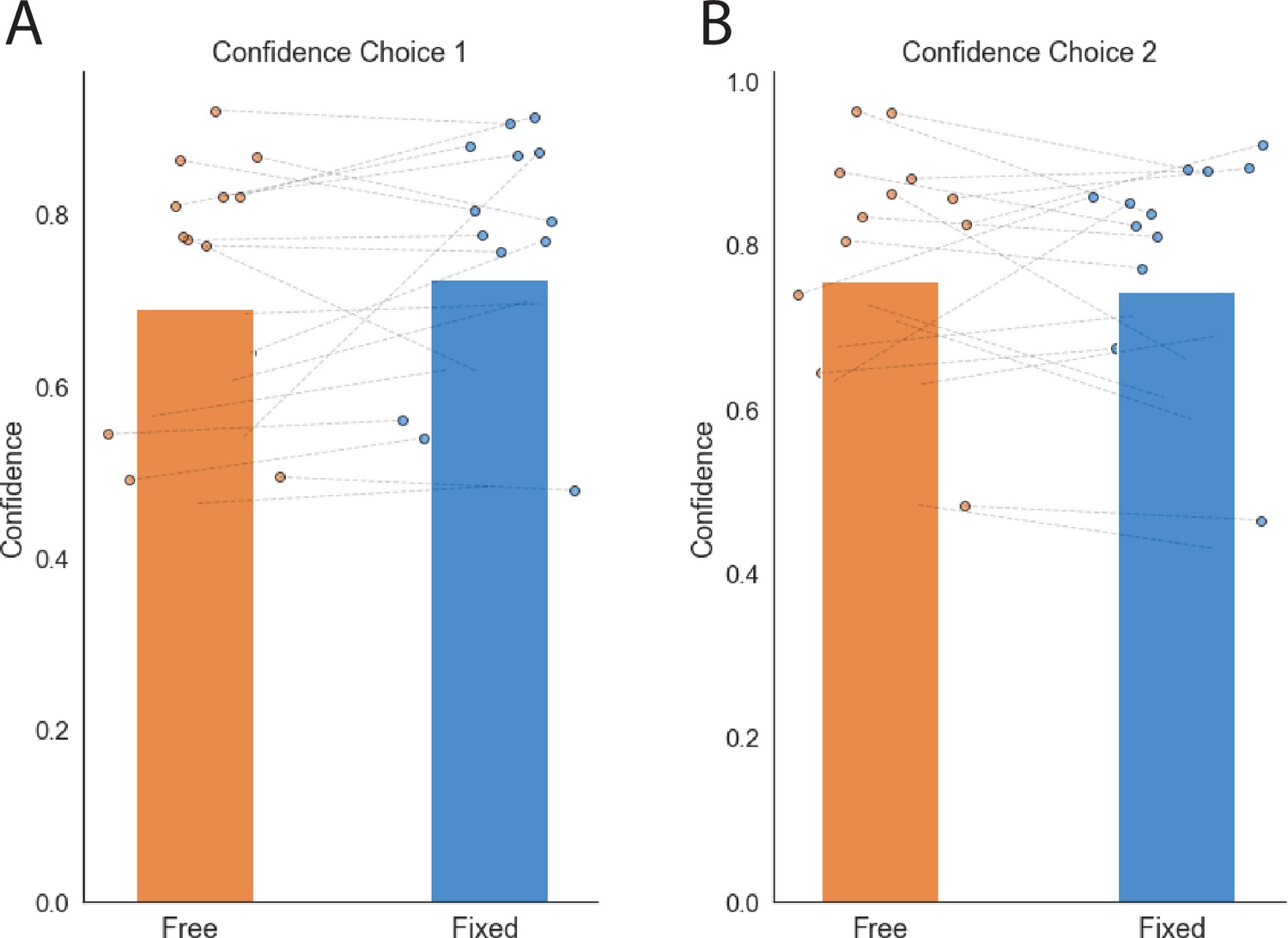
Confidence ratings experiment 2.
Each dot represents a single participant. The segmented lines connect the same participant in both conditions.
Figure 5 with 4 supplements
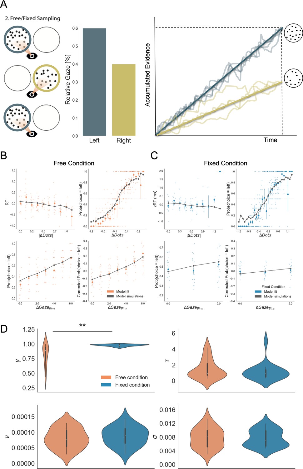
Gaze impacted evidence accumulation (for the 2nd choice) more strongly in the free than in the fixed sampling condition.
(A) Free and fixed sampling condition trials were fitted separately using a Gaze-weighted Linear Accumulator Model (GLAM). In this model there are two independent accumulators for each option (left and right) and the decision is made once one of them reaches a threshold. Accumulation rate was modulated by gaze times, when gaze bias parameter is lower than 1 (γ < 1). In that case, the accumulation rate will be discounted depending on γ and the relative gaze time to the items, within the trials. Gaze information from the free sampling trials, and presentation times from the fixed sampling trials were used to fit the models. The panel depicts an example trial: patch sampling during phase 2 (left panel) is used to estimate the relative gaze for that trial (central panel), and the resulting accumulation process (right panel) Notice GLAM ignores fixations dynamics and uses a constant accumulation term within trial (check Methods for further details). The model predicted the behaviour in free (B) and fixed (C) sampling conditions. The four panels present four relevant behavioural relationships comparing model predictions and overall participant behaviour: (top left) response time was faster (shorter RT) when the choice was easier (i.e. bigger differences in the number of dots between the patches); (top right) probability of choosing the left patch increased when the number of dots was higher in the patch at the left side (ΔDots = DotsLeft – DotsRight); (bottom left) the probability of choosing an alternative depended on the gaze difference (ΔGaze = gLeft – gRight); and (bottom right) the probability of choosing an item that was fixated longer than the other, corrected by the actual evidence ΔDots, depicted a residual effect of gaze on choice. Notice that in the free condition, the model predicted an effect of gaze on choice in a higher degree than in the fixed condition. Solid dots depict the mean of the data across participants in both conditions. Lighter dots present the mean value for each participant across bins. Solid grey lines show the average for model simulations. Data z-scored/binned for visualisation. (D) GLAM parameters fitted at participant level for free and fixed sampling conditions. Free sampling condition presented a higher gaze bias than fixed sampling, while no significant differences were found for the other parameters. γ: gaze bias; τ: evidence scaling; ν: drift term; σ: noise standard deviation. **: p < 0.01.
Figure 5—figure supplement 1
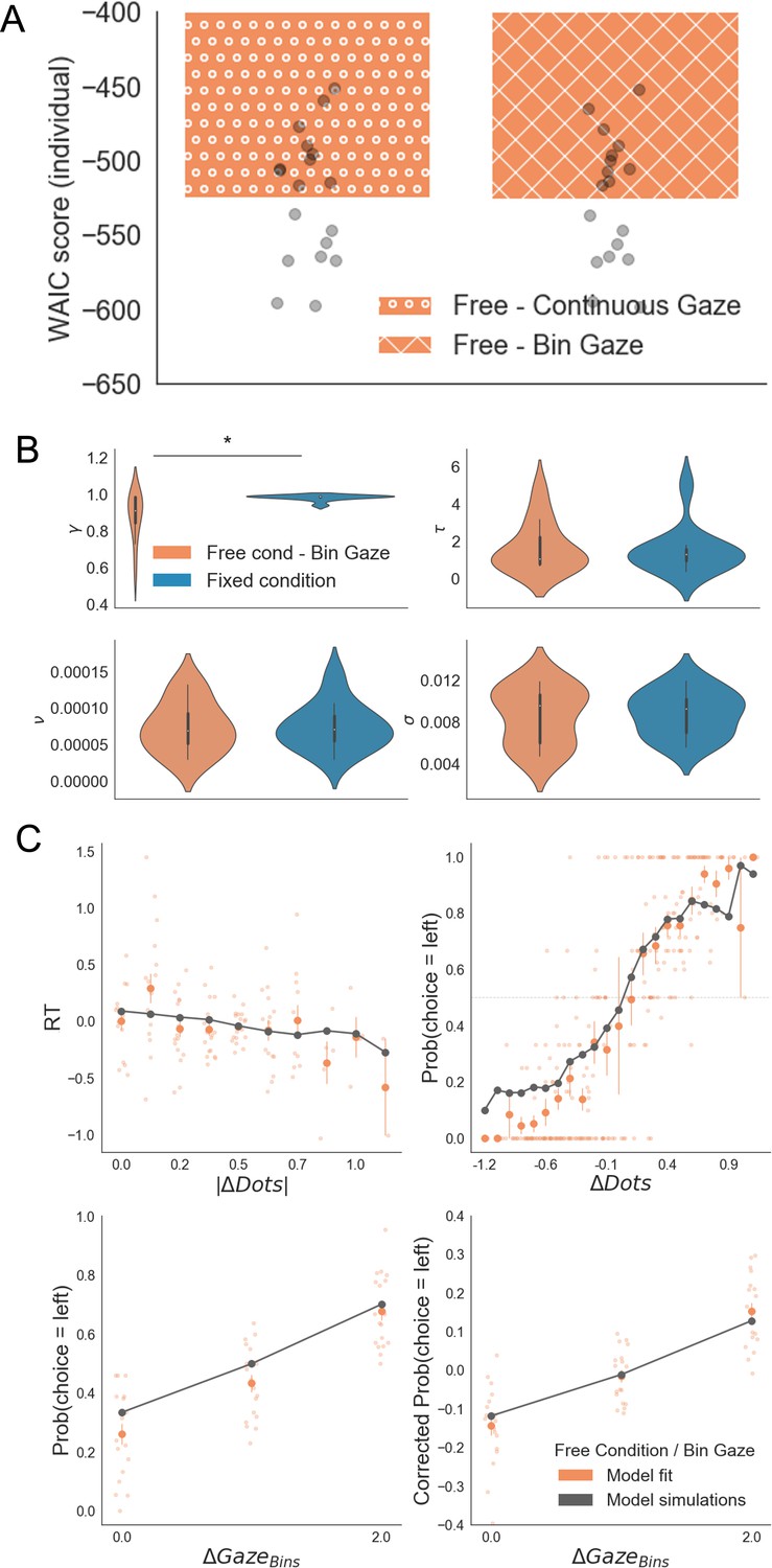
GLAM results with down-sampled gaze information in the free sampling condition.
To check whether the results reported in the main text are an artefact of the low variability in relative gaze in fixed sampling trials, we reduced the variability of free sampling trials to only 3 bins. This replicated the number of bins in the gaze allocation presented in our fixed-viewing trials. GLAM was fitted using these data. (A) Model comparison between the GLAM models in the free sampling condition fitted using original gaze data (continuous gaze) and the down sampled gaze information (bin gaze). We found no significant difference between the model fit scores in both cases (Mean WAICFree/Continuous = –524.58; Mean WAICFree/Bin = –525.12; t17 = 1.46, p = 0.16, ns). Model fitting was performed at a participant level. WAIC scores are presented using log scale. A higher log-score indicates a model with better predictive accuracy. (B) GLAM parameters resulting from Bin Gaze model fit. We replicated the findings in the main text, with a higher gaze bias (lower γ parameter) in the free sampling condition (Mean γ Free = 0.88, Mean γ Fixed = 0.98, t17 = –2.803; p < 0.05). No significant differences were found for the other parameters. γ: gaze bias; τ: evidence scaling; ν: drift term; σ: noise standard deviation. (C) The Bin Gaze model replicated the main behavioural relationships in a similar way to the original continuous gaze model. The four panels present four relevant behavioural relationships comparing model predictions and overall participant behaviour: (top left) responses time were faster (shorter RT) when the choice was easier (i.e. bigger differences in the number of dots between the patches); (top right) probability of choosing the left patch increased when the number of dots was higher in the patch on the left side (ΔDots = DotsLeft – DotsRight); (bottom left) the probability of choosing an alternative depended on the gaze difference (ΔGaze = gLeft – gRight); and (bottom right) the probability of choosing an item that was fixated longer than the other, corrected by the actual evidence (ΔDots), depicted a residual effect of gaze on choice. Solid dots depict the mean of the data across participants. Lighter dots present the mean value for each participant across bins. Solid grey lines show the average for model simulations. Data are binned for visualization. *: p < 0.05.
Figure 5—figure supplement 2
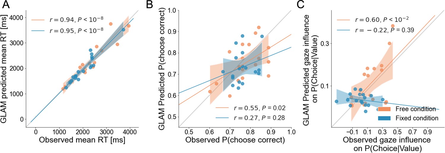
Individual out-of-sample GLAM predictions for behavioural measures in free and fixed sampling conditions.
The correlations between observed data and predictions of the model for individual (A) mean RT, (B) the probability of choosing the correct patch, and (C) the gaze influence in choice probability are presented. In the fixed sampling condition, the correlation between the performance (probability of correct) of individual participants and the model predictions was found not statistically significant, indicating the model was not completely accurate in predicting participant-level performance. However, the model captures group-level performance (as depicted in Figure 5C), since predicted trials had higher than chance accuracy and a similar range of performance as observed trials (accuracy is between 0.6–0.9 for observed and predicted). Regarding the gaze influence measure (residual effect of gaze on choice, once the effect of evidence is accounted for), the free sampling model predicts this effect significantly at the participant level, but the fixed sampling model did not. Since in the fixed sampling model, in practical terms there is no gaze bias (γ ≈1), we expected the model would have trouble predicting any residual gaze influence. Dots depict the average of observed and predicted measures for each participant. In the free sampling condition the model prediction correlated significantly with observed accuracy and gaze influence, at the participant-level. Lines depict the slope of the correlation between observations and predictions. Dots indicate the average measure for each participant’s observed and predicted data. Mean 95% confidence intervals are represented by the shadowed region. All model predictions are simulated using parameters estimated from individual fits for even-numbered trials.
Figure 5—figure supplement 3
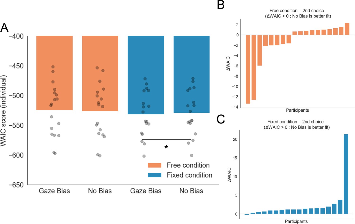
GLAM model comparison for free and fixed sampling conditions.
(A) WAIC scores for free and fixed sampling models did not report significant difference in fit between the conditions (mean WAICFree = –524.58; mean WAICFixed = –531.472; t17 = 1.33, p = 0.19, ns). As an additional check, we fitted new models for both conditions without the gaze bias (no bias, γ = 1). We found that in the fixed gaze condition, the no bias model was the most parsimonious model (Mean WAICFixed/GazeBias = –531.472; Mean WAICFixed/NoBias = –528.98; t17 = –2.197, p < 0.05). No differences were found between the gaze bias and no bias models in the free sampling condition (Mean WAICFree/GazeBias = –524.58; Mean WAICFree/NoBias = –526.23; t17 = 1.537, p = 0.14, ns). (B–C) Differences in WAIC score magnitudes between Gaze Bias – No Bias (ΔWAIC) models were calculated for each individual participant and experimental condition. This corroborated that the No Bias model has a better fit in the fixed sampling condition only (C). WAIC scores are presented using log scale. A higher log-score indicates a model with better predictive accuracy. *: p < 0.05.
Figure 5—figure supplement 4
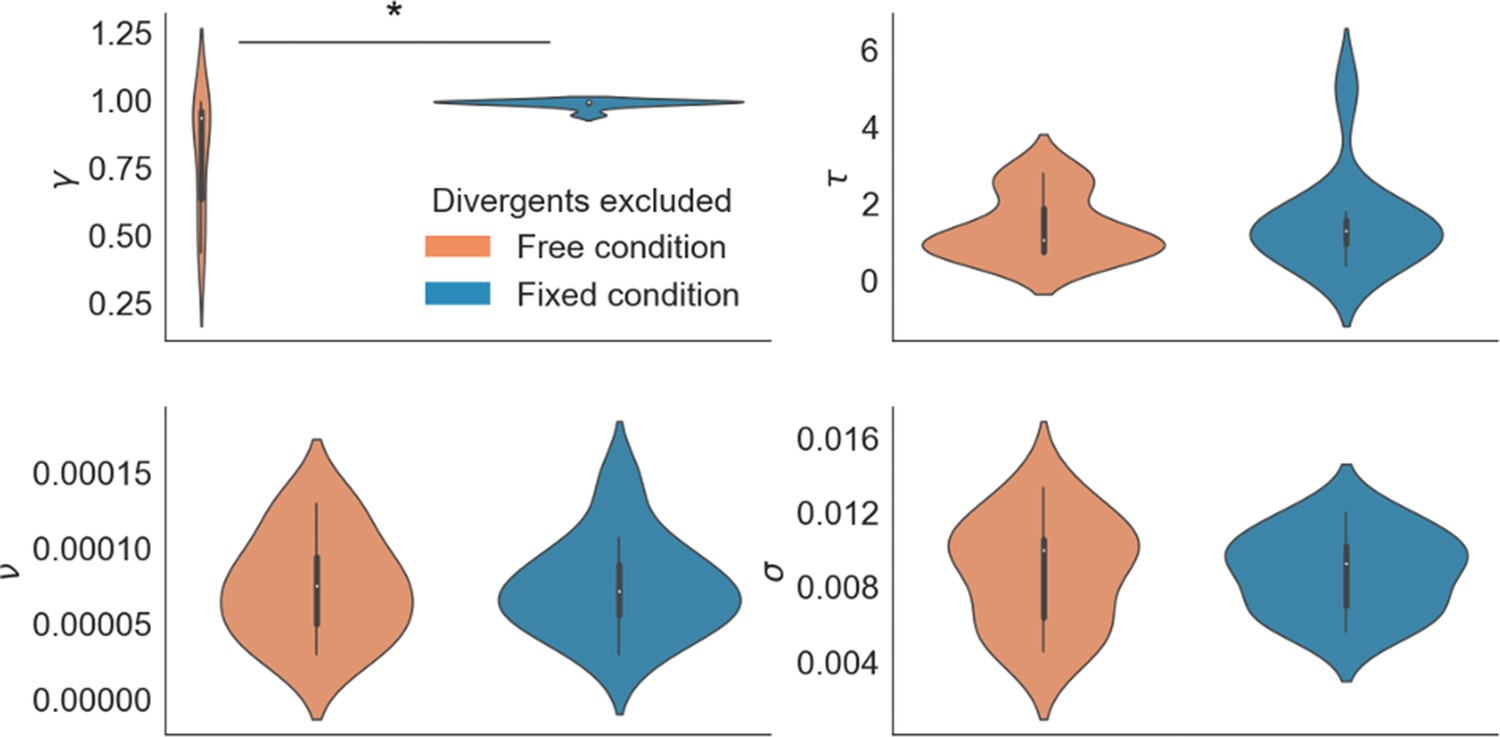
GLAM parameters for free and fixed sampling conditions.
Participants for which parameter estimation did not converge were removed from the analysis (7 participants). The results reported in the main text were still observed: a higher gaze bias (lower γ parameter) in the free sampling condition (Mean γ Free = 0.792, Mean γ Fixed = 0.982, t17 = –3.002; p < 0.05). No significant differences were found for the other parameters. γ: gaze bias; τ: evidence scaling; ν: drift term; σ: noise standard deviation. *: p < 0.05.
Appendix 4—figure 1
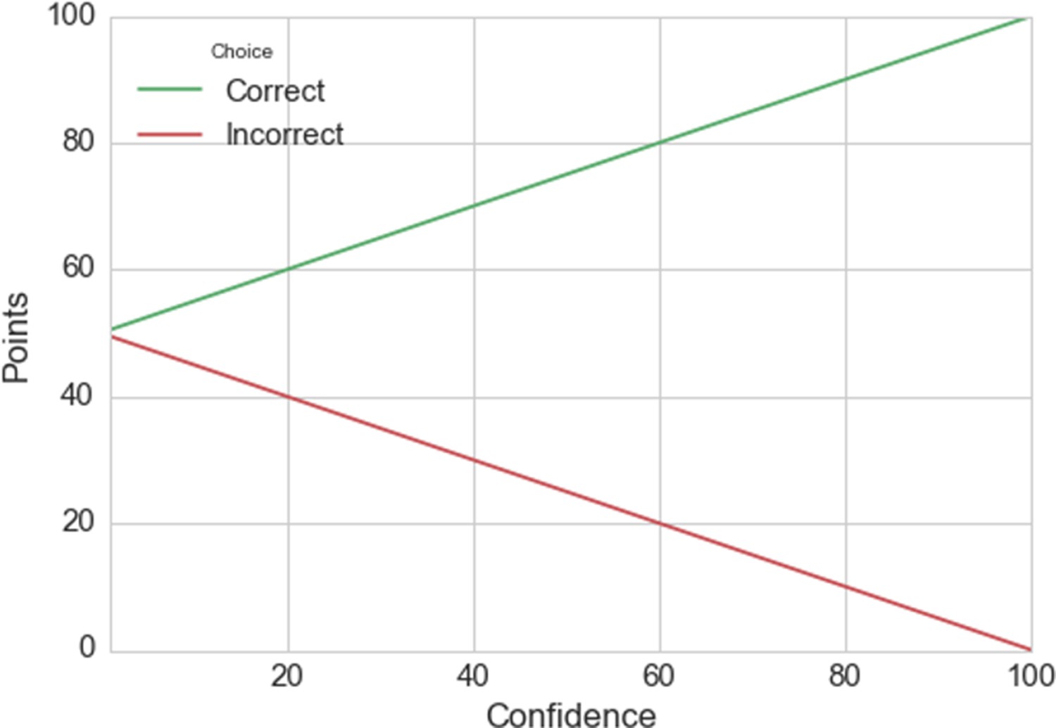
Linear scoring rule.
Appendix 5—figure 1
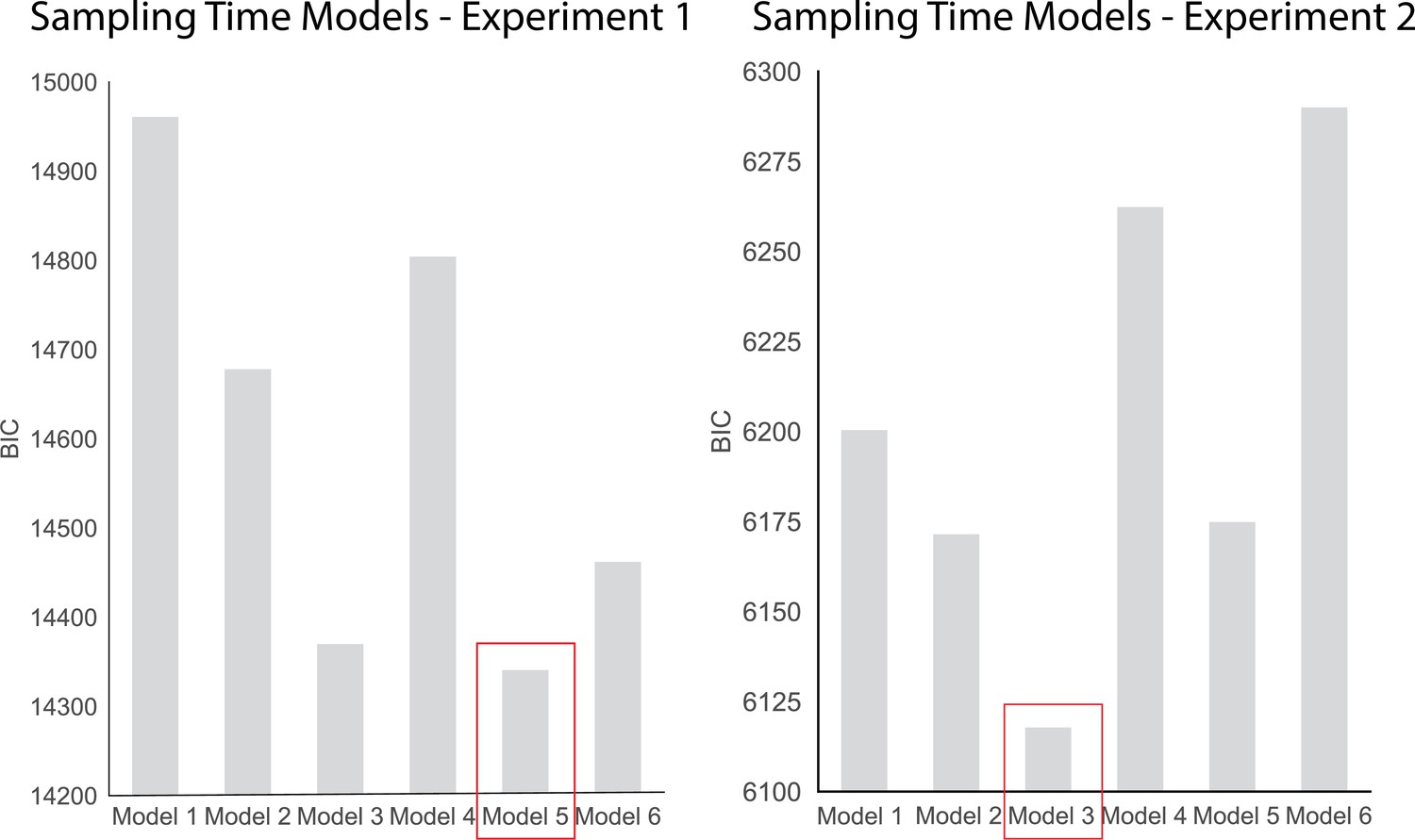
BIC comparison of the sampling time models for experiments 1 and 2.
Appendix 5—figure 2
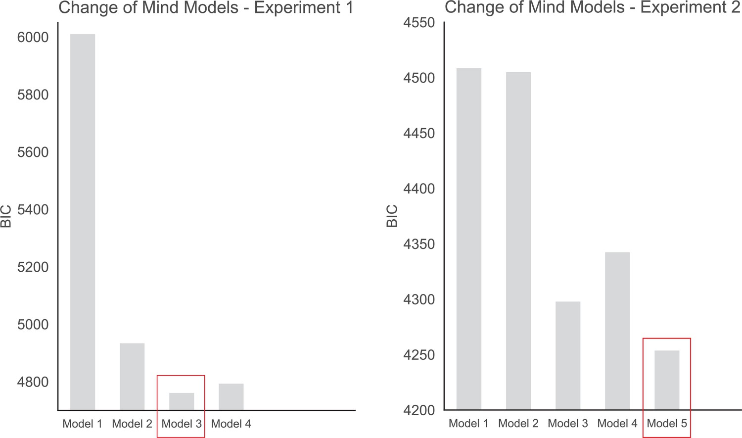
BIC comparison of the change of mind models for experiments 1 and 2.
Model 3 fit the data from experiment 1 the best (BIC = 4760.8), whereas Model 5 was the best fit for the data in experiment 2 (BIC = 4251.7).
Tables
Appendix 1—table 1
Hierarchical Regression Model Predicting Sampling Time Difference, Experiment 1.
| Predictor | Coefficient | SE | t-value | DF | p-value |
|---|---|---|---|---|---|
| Intercept | –0.27 | 0.03 | –8.48 | 26.28 | < 0.0001 |
| Choice | 0.51 | 0.05 | 9.64 | 26.87 | < 0.0001 |
| Dot Difference | 0.05 | 0.004 | 13.02 | 26.80 | < 0.0001 |
| Confidence | –0.08 | 0.03 | –2.88 | 28.74 | 0.007 |
| Choice x Confidence | 0.19 | 0.04 | 5.26 | 26.59 | < 0.0001 |
Appendix 1—table 2
Hierarchical Regression Model Predicting Sampling Time Difference, Experiment 2.
| Predictor | Coefficient | SE | t-value | DF | p-value |
|---|---|---|---|---|---|
| Intercept | –0.15 | 0.06 | –2.63 | 16.94 | 0.017 |
| Choice | 0.30 | 0.10 | 2.90 | 16.75 | 0.01 |
| Dot Difference | 0.04 | 0.005 | 9.21 | 68.14 | < 0.0001 |
| Confidence | –0.09 | 0.04 | –2.43 | 18.31 | 0.03 |
| Choice x Confidence | 0.21 | 0.05 | 4.29 | 32.00 | 0.0005 |
Appendix 2—table 1
Hierarchical Logistic Regression Model Predicting Change of Mind, Experiment 1.
| Predictor | Coefficient | SE | z-value | p-value |
|---|---|---|---|---|
| Intercept | –1.18 | 0.21 | –5.65 | < 0.0001 |
| Sampling Bias | –1.24 | 0.08 | –11.0 | < 0.0001 |
| Dot Difference | –0.24 | 0.11 | –3.06 | 0.002 |
| Confidence | –0.58 | 0.06 | –10.12 | < 0.0001 |
Appendix 2—table 2
Hierarchical Logistic Regression Model Predicting Change of Mind, Experiment 2.
| Predictor | Coefficient | SE | z-value | p-value |
|---|---|---|---|---|
| Intercept | –1.05 | 0.28 | –3.76 | 0.0002 |
| Sampling Bias | –1.39 | 0.19 | –7.20 | < 0.0001 |
| Dot Difference | –0.25 | 0.10 | –2.66 | 0.008 |
| Confidence | –0.57 | 0.07 | –8.73 | < 0.0001 |
| Fixed Sampling | –0.09 | 0.14 | –0.61 | 0.54 |
| Sampling Bias x Fixed Sampling | 1.30 | 0.19 | 6.77 | < 0.0001 |
Appendix 5—table 1
Sampling Time Models.
| Models | Formula |
|---|---|
| 1 | Sampling Time Difference ~ (β0 + β1[Choice] + ε) |
| 2 | Sampling Time Difference ~(β0 + β1[Dot Difference] + ε) |
| 3 | Sampling Time Difference ~(β0 + β1[Choice] + β2[Dot Difference] + ε) |
| 4 | Sampling Time Difference ~ (β0 + β1[Choice] + β2[Confidence] + β3[Choice * Confidence] + ε) |
| 5 | Sampling Time Difference ~(β0 + β1[Choice] + β2[Dot Difference] + β3[Confidence] + β4[Choice * Confidence] + ε) |
| 6 | Sampling Time Difference ~(β0 + β1[Choice] + β2[Dot Difference] + β3[Confidence] + β4[Reaction Time] + β5[Choice * Confidence] + β6[Choice * Reaction Time] + ε) |
Additional files
Download links
A two-part list of links to download the article, or parts of the article, in various formats.
Downloads (link to download the article as PDF)
Open citations (links to open the citations from this article in various online reference manager services)
Cite this article (links to download the citations from this article in formats compatible with various reference manager tools)
Humans actively sample evidence to support prior beliefs
eLife 11:e71768.
https://doi.org/10.7554/eLife.71768


