Modeling the spatiotemporal spread of beneficial alleles using ancient genomes
Figures
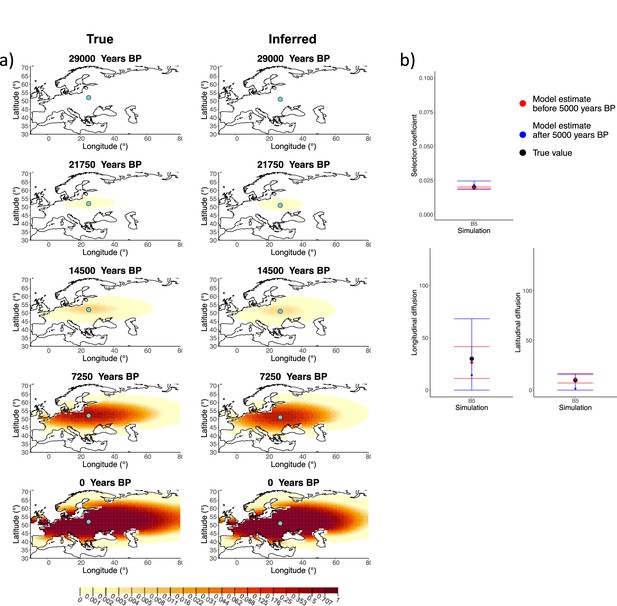
Comparison of true and inferred allele frequency dynamics for simulation B5.
(a) Comparison of true and inferred allele frequency dynamics for a simulation with diffusion and no advection (B5). The green dot corresponds to the origin of the allele. The parameter values used to generate the frequency surface maps are summarized in Appendix 2—table 1. (b) Comparison of true parameter values and model estimates. Whiskers represent 95% confidence intervals.
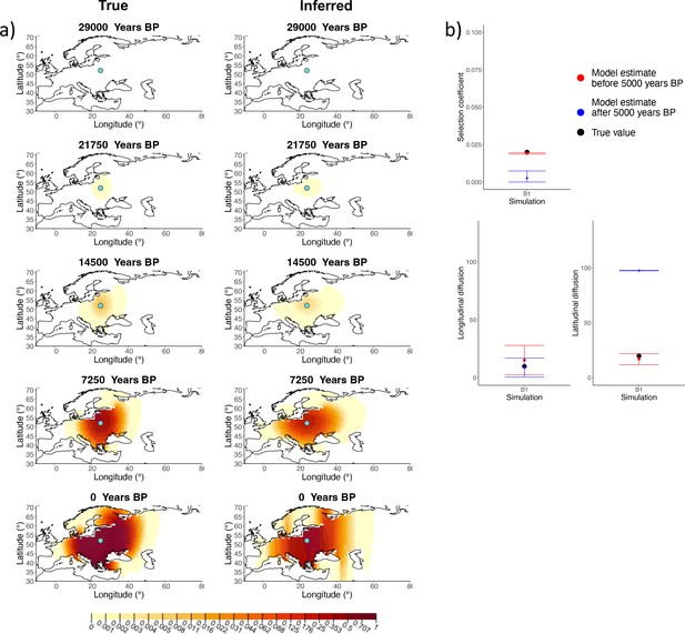
Comparison of true and inferred allele frequency dynamics for simulation B1.
(a) Comparison of true and inferred allele frequency dynamics for simulation B1. The green dot corresponds to the origin of the allele. The parameter values used to generate the frequency surface maps are summarized in Appendix 2—table 1. (b) Comparison of true parameter values and model estimates. Whiskers represent 95% confidence intervals.
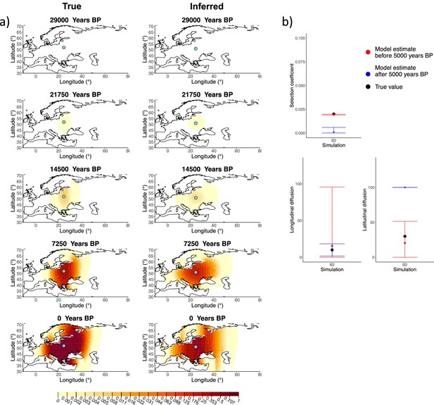
Comparison of true and inferred allele frequency dynamics for simulation B2.
(a) Comparison of true and inferred allele frequency dynamics for simulation B2. The green dot corresponds to the origin of the allele. The parameter values used to generate the frequency surface maps are summarized in Appendix 2—table 1. (b) Comparison of true parameter values and model estimates. Whiskers represent 95% confidence intervals.
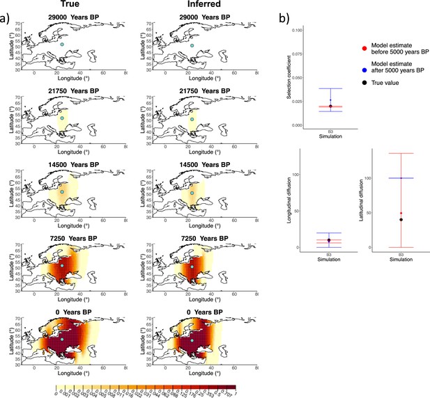
Comparison of true and inferred allele frequency dynamics for simulation B3.
(a) Comparison of true and inferred allele frequency dynamics for simulation B3. The green dot corresponds to the origin of the allele. The parameter values used to generate the frequency surface maps are summarized in Appendix 2—table 1. (b) Comparison of true parameter values and model estimates. Whiskers represent 95% confidence intervals.
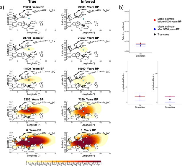
Comparison of true and inferred allele frequency dynamics for simulation B4.
(a) Comparison of true and inferred allele frequency dynamics for simulation B4. The green dot corresponds to the origin of the allele. The parameter values used to generate the frequency surface maps are summarized in Appendix 2—table 1. (b) Comparison of true parameter values and model estimates. Whiskers represent 95% confidence intervals.
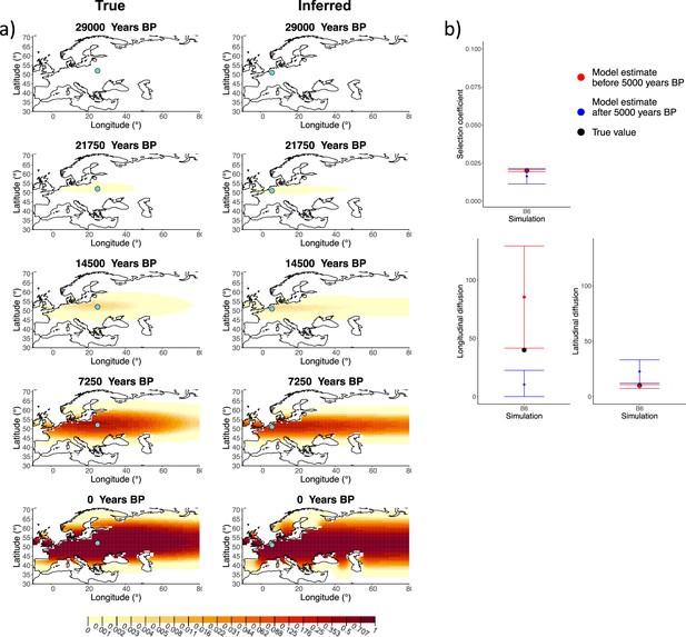
Comparison of true and inferred allele frequency dynamics for simulation B6.
(a) Comparison of true and inferred allele frequency dynamics for simulation B6. The green dot corresponds to the origin of the allele. The parameter values used to generate the frequency surface maps are summarized in Appendix 2—table 1. (b) Comparison of true parameter values and model estimates. Whiskers represent 95% confidence intervals.
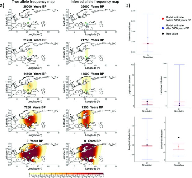
Comparison of true allele frequency dynamics for simulation B1 and those inferred by the model C.
(a) Comparison of true allele frequency dynamics for simulation B1 and those inferred by the model C. The green dot shows the origin of the derived allele and the cross represents the location of the first individual that carried it. (b) Comparison of true parameter values and model estimates. Whiskers represent 95% confidence intervals.
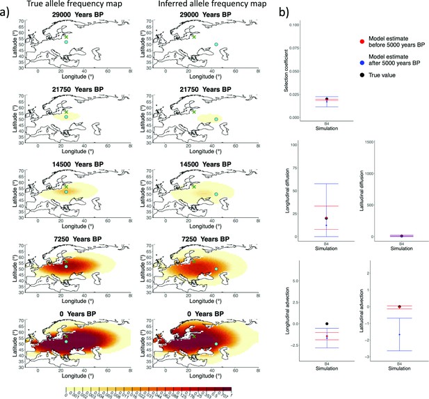
Comparison of true allele frequency dynamics for simulation B4 and those inferred by the model C.
(a) Comparison of true allele frequency dynamics for simulation B4 and those inferred by the model C. The green dot corresponds to the origin of the allele, and the cross represents the first sample having the derived variant. (b) Comparison of true parameter values and model estimates. Whiskers represent 95% confidence intervals.
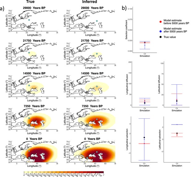
Comparison of true and inferred allele frequency dynamics for simulation C4.
(a) Comparison of true and inferred allele frequency dynamics for one of the simulations including advection (C4). The green dot corresponds to the origin of the allele. The parameter values used to generate the frequency surface maps are summarized in Appendix 2—table 2. (b) Comparison of true parameter values and model estimates. Whiskers represent 95% confidence intervals.
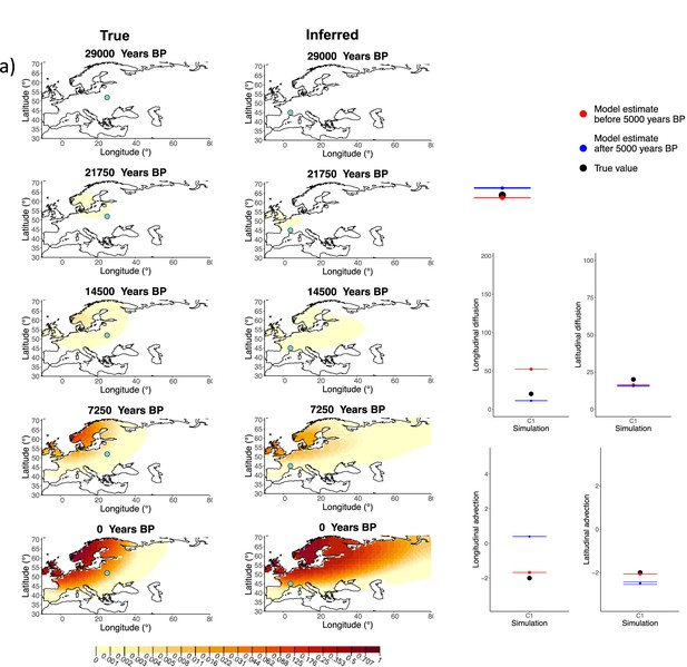
Comparison of true and inferred allele frequency dynamics for simulation C1.
(a) Comparison of true and inferred allele frequency dynamics for one of the simulations including advection (C1). The green dot corresponds to the origin of the allele. The parameter values used to generate the frequency surface maps are summarized in Appendix 2—table 2. (b) Comparison of true parameter values and model estimates. Whiskers represent 95% confidence intervals.
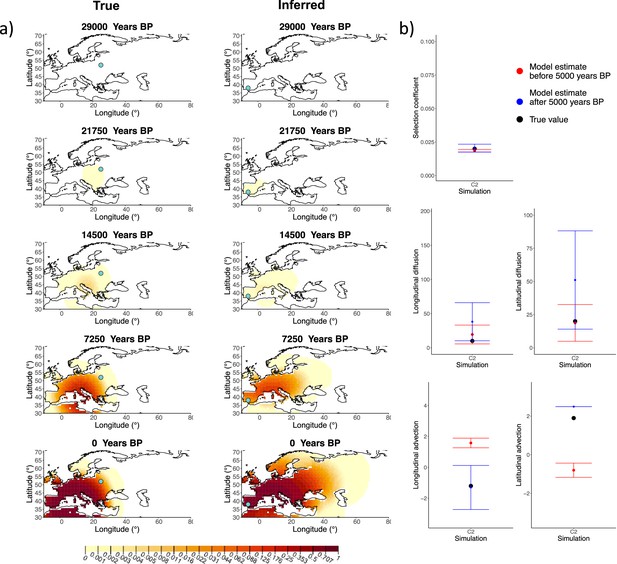
Comparison of true and inferred allele frequency dynamics for simulation C2.
(a) Comparison of true and inferred allele frequency dynamics for one of the simulations including advection (C2). The green dot corresponds to the origin of the allele. The parameter values used to generate the frequency surface maps are summarized in Appendix 2—table 2. (b) Comparison of true parameter values and model estimates. Whiskers represent 95% confidence intervals.
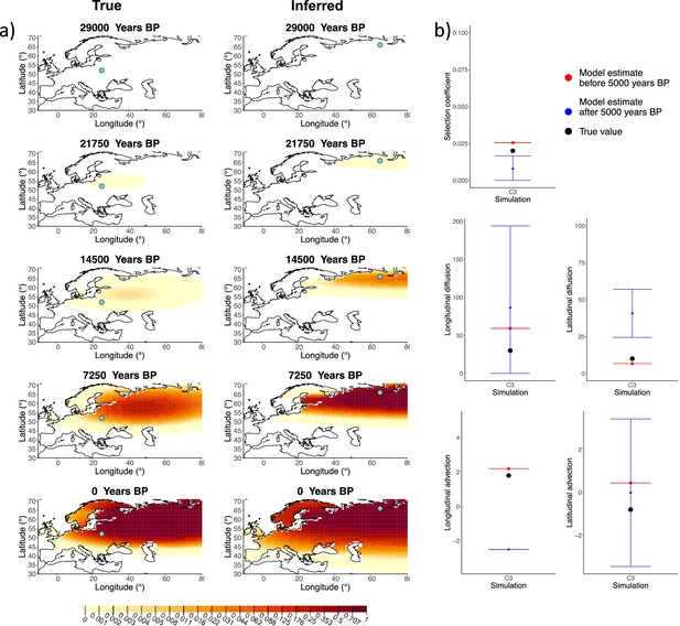
Comparison of true and inferred allele frequency dynamics for simulation C3.
(a) Comparison of true and inferred allele frequency dynamics for one of the simulations including advection (C3). The green dot corresponds to the origin of the allele. The parameter values used to generate the frequency surface maps are summarized in Appendix 2—table 2. (b) Comparison of true parameter values and model estimates. Whiskers represent 95% confidence intervals.
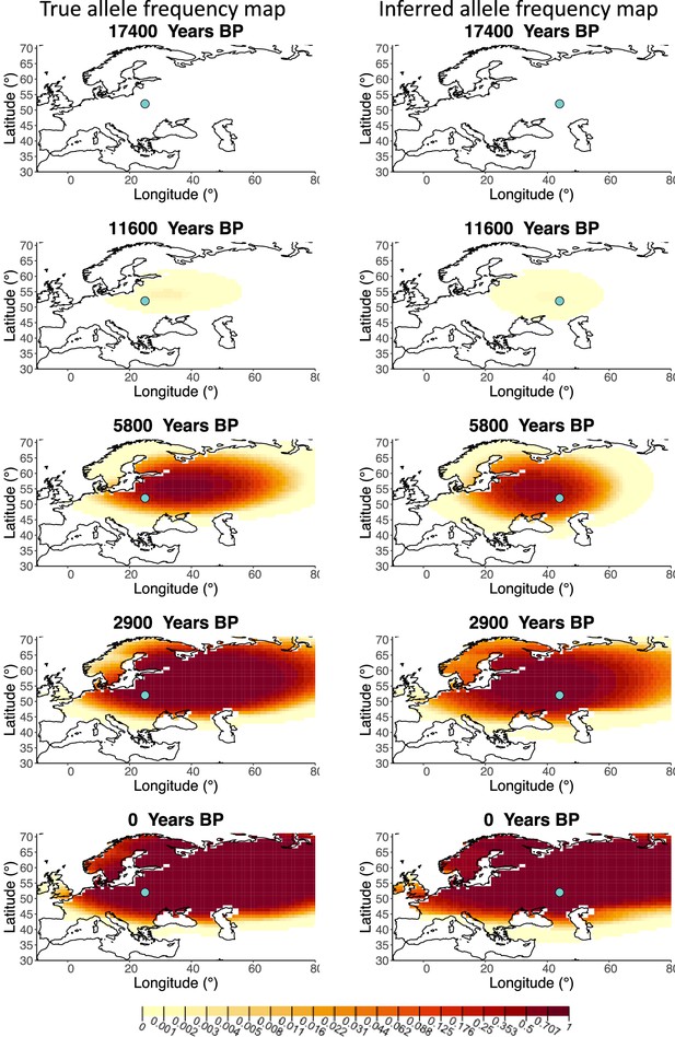
Comparison of true allele frequency map and map generated using ‘intermediate 75%/25%’ clustering scheme.
Left: allele frequency map generated using true parameter values. Right: allele frequency map generated using parameter estimates for ‘intermediate 75%/25%’ clustering scheme. Parameter values used to generate the maps are summarized in Appendix 2—table 3.
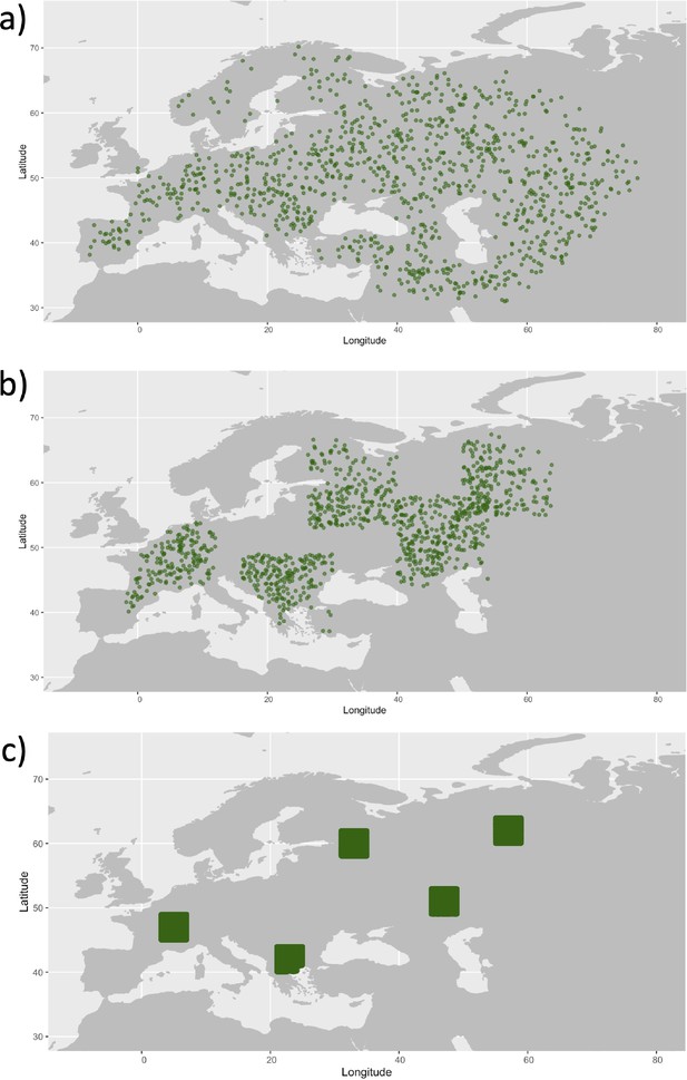
Examples of spatial sampling scenarios for each of the three clustering schemes.
We chose five locations and increasingly restricted the area where we allowed the individuals to be sampled. (a) Map showing homogeneous sampling scheme in which we did not impose any spatial restrictions of individuals sampled. (b) Intermediate sampling scheme with the region restricted to 7° in each cardinal direction from each of the chosen locations. (c) Extreme sampling scheme with the sampling region restricted to 2° in each cardinal direction from the chosen locations.
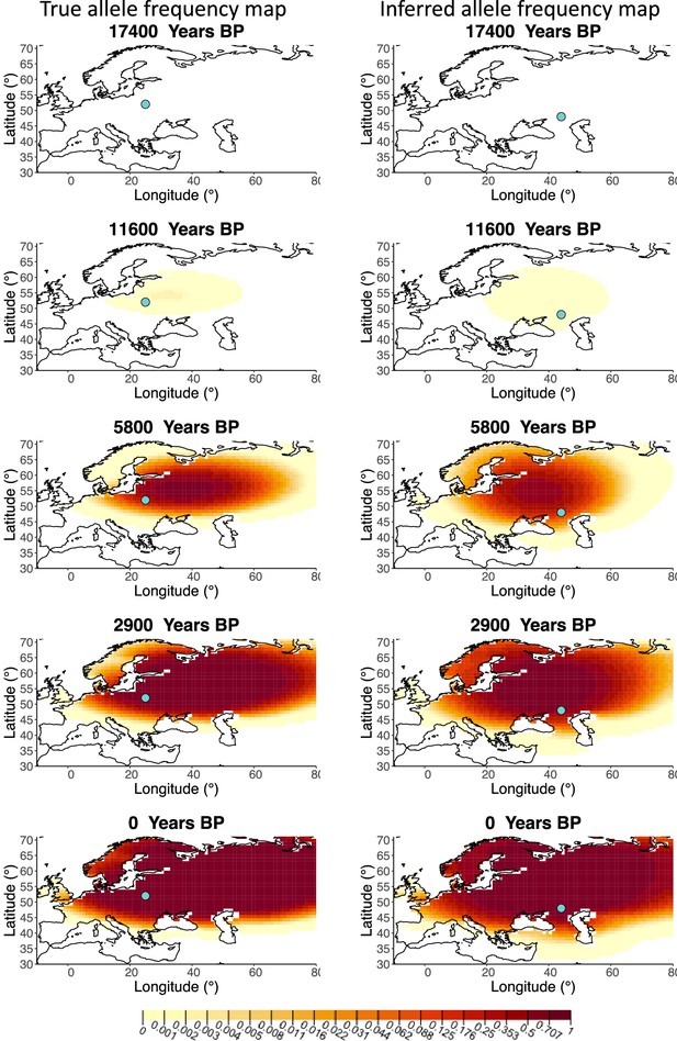
Allele frequency map generated using true parameter values and using parameter estimates for ‘homogeneous 75%/25%’ clustering scheme.
Left: allele frequency map generated using true parameter values. Right: allele frequency map generated using parameter estimates for ‘homogeneous 75%/25%’ clustering scheme. Parameter values used to generate the maps are summarized in Appendix 2—table 3.
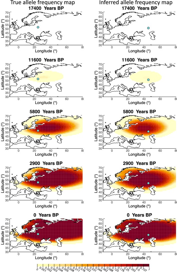
Allele frequency map generated using true parameter values and using parameter estimates for ‘homogeneous 50%/50%’ clustering scheme.
Left: allele frequency map generated using true parameter values. Right: allele frequency map generated using parameter estimates for ‘homogeneous 50%/50%’ clustering scheme. Parameter values used to generate the maps are summarized in Appendix 2—table 3.

Allele frequency map generated using true parameter values and using parameter estimates for ‘homogeneous 25%/75%’ clustering scheme.
Left: allele frequency map generated using true parameter values. Right: allele frequency map generated using parameter estimates for ‘homogeneous 25%/75%’ clustering scheme. Parameter values used to generate the maps are summarized in Appendix 2—table 3.
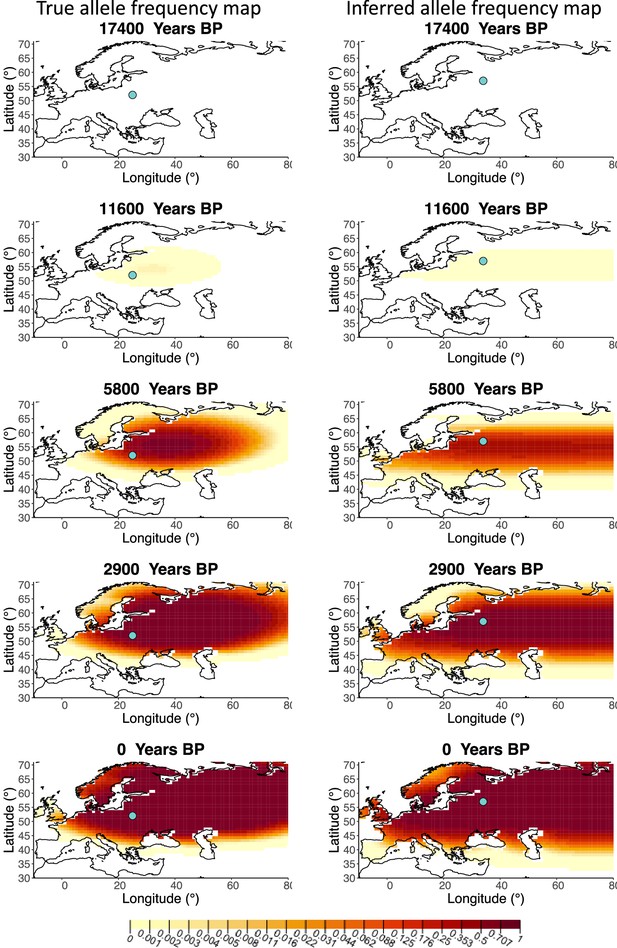
Allele frequency map generated using true parameter values and using parameter estimates for ‘intermediate 50%/50%’ clustering scheme.
Left: allele frequency map generated using true parameter values. Right: allele frequency map generated using parameter estimates for ‘intermediate 50%/50%’ clustering scheme. Parameter values used to generate the maps are summarzsed in Appendix 2—table 3.
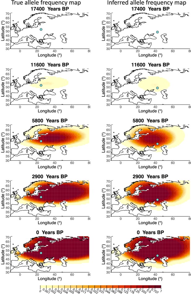
Allele frequency map generated using true parameter values and using parameter estimates for ‘intermediate 25%/75%’ clustering scheme.
Left: allele frequency map generated using true parameter values. Right: allele frequency map generated using parameter estimates for ‘intermediate 25%/75%’ clustering scheme. Parameter values used to generate the maps are summarized in Appendix 2—table 3.
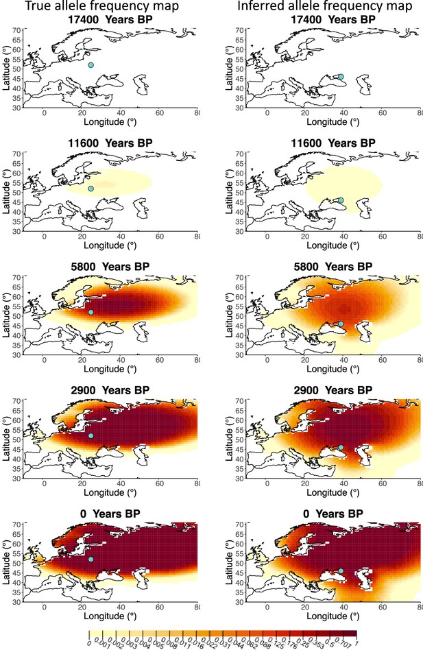
Allele frequency map generated using true parameter values and using parameter estimates for ‘extreme 75%/25%’ clustering scheme.
Left: allele frequency map generated using true parameter values. Right: allele frequency map generated using parameter estimates for ‘extreme 75%/25%’ clustering scheme. Parameter values used to generate the maps are summarzsed in Appendix 2—table 3.
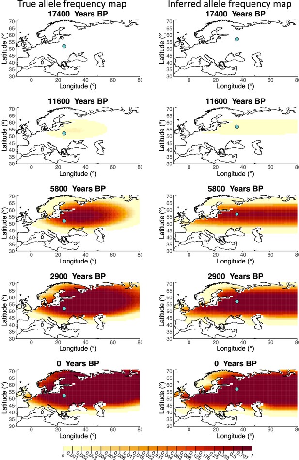
Allele frequency map generated using true parameter values and using parameter estimates for ‘extreme 50%/50%’ clustering scheme.
Left: allele frequency map generated using true parameter values. Right: allele frequency map generated using parameter estimates for ‘extreme 50%/50%’ clustering scheme. Parameter values used to generate the maps are summarized in Appendix 2—table 3.
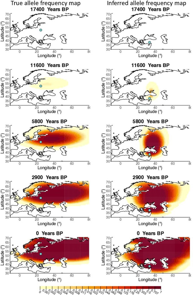
Allele frequency map generated using true parameter values and using parameter estimates for ‘extreme 25%/75%’ clustering scheme.
Left: allele frequency map generated using true parameter values. Right: allele frequency map generated using parameter estimates for ‘extreme 25%/75%’ clustering scheme. Parameter values used to generate the maps are summarized in Appendix 2—table 3.
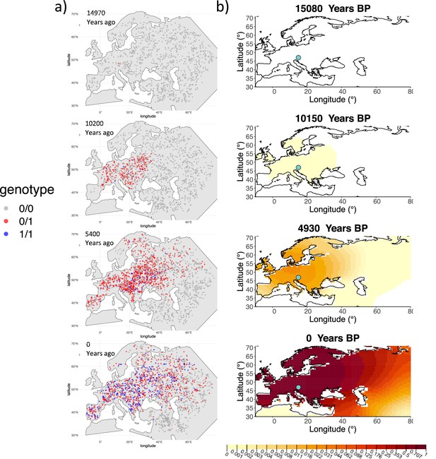
Comparison of an individual-based simulation and allele frequency dynamics inferred by the diffusion model.
(A) Individual-based simulation of an allele that arose in Central Europe 15,000 years ago with a selection coefficient of 0.03. Each dot represents a genotype from a simulated genome. To avoid overplotting, only 1000 out of the total 20,000 individuals in the simulation in each time point are shown for each genotype category. (B) Allele frequency dynamics inferred by the diffusion model on the individual-based simulation to the left, after randomly sampling 1040 individuals from the simulation and performing pseudohaploid genotype sampling on them. The ages of sampled individuals were log-uniformly distributed. The estimated parameter values of the fitted model are shown in Appendix 2—table 4.
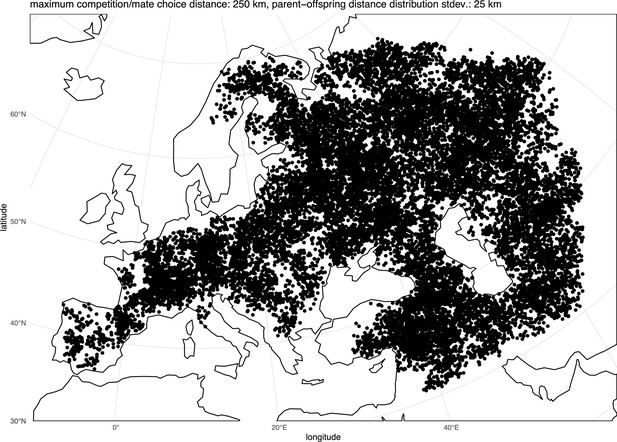
Distribution of individuals across the map under neutrality, showing the tendency of individuals to cluster together.
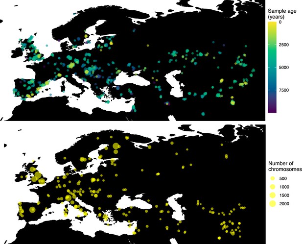
Locations of samples used to model the spread of the rs4988235(T) allele.
The upper panel shows the spatiotemporal locations of ancient individuals, and the bottom panel represents the locations of present-day individuals.
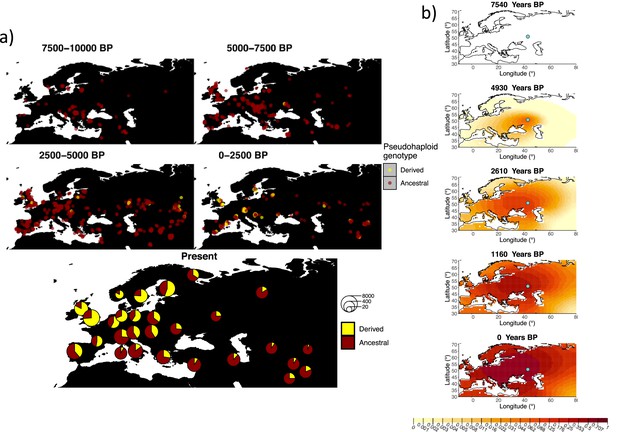
Allele frequency dynamics of rs4988235(T).
(a) Top: pseudohaploid genotypes of ancient samples at the rs4988235 SNP in different periods. Yellow corresponds to the rs4988235(T) allele. Bottom: allele frequencies of present-day samples represented as pie charts. The size of the pie charts corresponds to the number of available sequences in each region. (b) Inferred allele frequency dynamics of rs4988235(T). The green dot indicates the inferred geographic origin of the allele.

Inferred frequency dynamics of rs4988235(T) using the allele age that was inferred in Albers and McVean, 2020.

Inferred frequency dynamics of rs4988235(T) when the origin of the allele is moved 10° west from the original estimate.

Inferred frequency dynamics of rs4988235(T) when the origin of the allele is moved 10° east from the original estimate.

Inferred frequency dynamics of rs4988235(T) when the origin of the allele is moved 10° north from the original estimate.
.

Inferred frequency dynamics of rs4988235(T) when the origin of the allele is moved 10° south from the original estimate.

Inferred frequency dynamics of rs4988235(T) forcing the geographic origin of the allele to be at the location inferred in Itan et al., 2009.

Inferred frequency dynamics of rs4988235(T) assuming the allele age to be the lower end of the 95% credible interval for the start of selection onset inferred in Itan et al., 2009.

Inferred frequency dynamics of rs4988235(T) assuming the allele age to be the higher end of the 95% credible interval for the start of selection onset inferred in Itan et al., 2009.
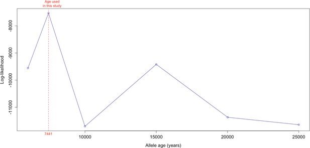
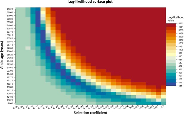
Log-likelihood values for model runs using different ages of the rs4988235(T) allele as input, with the age inferred by Itan et al., 2009 we use as fixed input highlighted in red.
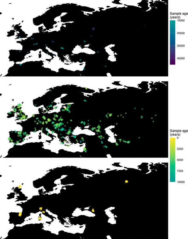
Spatiotemporal sampling locations of sequences used to model the rs1042602(A) allele in Western Eurasia.
Upper panel: ancient individuals dated as older than 10,000 years ago. Middle panel: ancient individuals dated as younger than 10,000 years ago. Bottom panel: present-day individuals from the Human Genome Diversity Panel (HGDP).
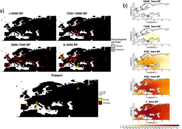
Allele frequency dynamics of rs1042602(A).
(a) Top: pseudohaploid genotypes of ancient samples of the rs1042602 in different periods. Yellow corresponds to the A allele. Bottom: diploid genotypes of present-day samples. (b) Inferred allele frequency dynamics of rs1042602(A). The green dot corresponds to the inferred geographic origin of the allele.

Inferred frequency dynamics of rs1042602(A) when the origin of the allele is moved 10° east from the original estimate.

Inferred frequency dynamics of rs1042602(A) when the origin of the allele is moved 10° north from the original estimate.

Inferred frequency dynamics of rs1042602(A) when the origin of the allele is moved 10° south from the original estimate.

Inferred frequency dynamics of rs1042602(A) assuming the allele age to be the lower end of the 95% confidence interval for the allele age inferred in Albers and McVean, 2020.

Frequency dynamics of rs1042602(A) assuming the allele age to be the higher end of the 95% confidence interval for the allele age inferred in Albers and McVean, 2020.
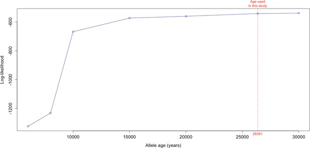
Log-likelihood values for model runs using different ages of the rs1042602(A) allele as input, with the age inferred by Albers and McVean, 2020 we use as fixed input highlighted in red.
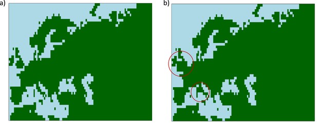
Maps showing areas where diffusion in the model is allowed (green) and where it is forbidden (blue).
(a) Map without land bridges. (b) Map containing land bridges indicated with red circles.
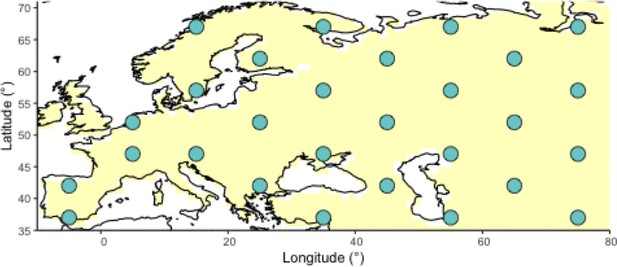
Geographic locations for points used as potential origins of the allele at the initialization of the simulated annealing optimization algorithm.
Note that, after initialization, the algorithm can continuously explore any points on the map grid that are not necessarily included in this point set.
Tables
Parameter values used to generate simulations using numerical solutions to Equation 3 compared to parameter estimates assuming model B.
The age of the allele was set to 29,000 years in all simulations. Columns named ‘long’ and ‘lat’ indicate the longitude and latitude of the geographic origin of the allele, respectively.
| Simulation | (km2/gen) | (km2/gen) | Long | Lat | ||
|---|---|---|---|---|---|---|
| True/pred (95% CI) | True/pred (95% CI) | True/pred (95% CI) | True/pred | True/pred | ||
| B1 | Sample age >5000 | 0.02/0.0192 (0.0187 to 0.0196) | 10/15.244 (2.5042 to 27.9828) | 20/16.963 (11.9263 to 21.9993) | 25/24 | 52/52 |
| Sample age <5000 | 0.02/0.0027 (0 to 0.0074) | 10/8.805 (0.5631 to 17.0468) | 20/97.432 (97.2566 to 97.6081) | – | – | |
| B2 | Sample age >5000 | 0.02/0.0193 (0.0189 to 0.0198) | 10/15.348 (0 to 95.5192) | 30/20.427 (0 to 51.514) | 25/25 | 52/51 |
| Sample age <5000 | 0.02/0.001 (0 to 0.0059) | 10/10.015 (1.6837 to 18.3472) | 30/100 (99.9933 to 100.0067) | – | – | |
| B3 | Sample age >5000 | 0.02/0.0196 (0.0191 to 0.02) | 10/8.149 (6.1551 to 10.143) | 40/49.432 (0 to 135.9428) | 25/24 | 52/51 |
| Sample age <5000 | 0.02/0.0265 (0.0145 to 0.0386) | 10/7.855 (0 to 19.751) | 40/100 (99.9933 to 100.0067) | – | – | |
| B4 | Sample age >5000 | 0.02/0.0188 (0.0188 to 0.0188) | 20/19.037 (19.0311 to 19.0435) | 10/19.254 (19.2439 to 19.2638) | 25/25 | 52/51 |
| Sample age <5000 | 0.02/0.0142 (0.0111 to 0.0173) | 20/17.354 (4.4083 to 30.2991) | 10/1.489 (0 to 18.5993) | – | – | |
| B5 | Sample age >5000 | 0.02/0.0196 (0.019 to 0.0202) | 30/26.409 (11.1997 to 41.6184) | 10/11.429 (7.1825 to 15.6759) | 25/27 | 52/51 |
| Sample age <5000 | 0.02/0.0215 (0.0183 to 0.0246) | 30/14.3 (0 to 68.176) | 10/1.554 (0 to 16.5985) | – | – | |
| B6 | Sample age >5000 | 0.02/0.0199 (0.0192 to 0.0206) | 40/85.415 (41.6058 to 129.2248) | 10/9.02 (7.2853 to 10.7538) | 25/6 | 52/51 |
| Sample age <5000 | 0.02/0.0163 (0.0112 to 0.0213) | 40/10.403 (0 to 22.533) | 10/22.623 (12.0841 to 33.1614) | – | – | |
Parameter values used to generate simulations using numerical solutions to Equation 4, compared to parameter estimates assuming model C.
The age of the allele was set to 29,000 years in all simulations. Columns named ‘long’ and ‘lat’ indicate the longitude and latitude of the geographic origin of the allele, respectively.
| Simulation | (km2/gen) | (km2/gen) | vx (km/gen) | vy (km/gen) | Long | Lat | ||
|---|---|---|---|---|---|---|---|---|
| True/pred (95% CI) | True/pred (95% CI) | True/pred (95% CI) | True/pred (95% CI) | True/pred (95% CI) | True/pred | True/pred | ||
| C1 | Sample age >5000 | 0.02/0.0189 (0.0188 to 0.0189) | 20/52.246 (52.2051 to 52.2872) | 20/16.373 (16.332 to 16.4139) | -2/-1.675 (-1.6771 to -1.6722) | -2/-2.067 (-2.0702 to -2.0639) | 25/4 | 52/45 |
| Sample age <5000 | 0.02/0.0231 (0.023 to 0.0233) | 20/11.086 (10.9286 to 11.2441) | 20/15.606 (15.3659 to 15.8467) | -2/0.399 (0.3946 to 0.4037) | -2/-2.491 (-2.5458 to -2.436) | – | – | |
| C2 | Sample age >5000 | 0.02/0.0185 (0.0176 to 0.0195) | 10/19.434 (5.6736 to 33.1952) | 20/18.727 (4.8938 to 32.5605) | -1.2/1.579 (1.2671 to 1.8905) | 1.9/-0.801 (-1.1684 to -0.4331) | 25/-6 | 52/38 |
| Sample age <5000 | 0.02/0.0205 (0.0175–0.0234) | 10/38.144 (10.3123 to 65.9749) | 20/51.094 (14.0489 to 88.1388) | -1.2/-1.299 (-2.7247 to 0.1266) | 1.9/2.493 (2.4929 to 2.4933) | – | – | |
| C3 | Sample age >5000 | 0.02/0.0255 (0.0254–0.0256) | 30/59.237 (59.1269 to 59.347) | 10/6.604 (6.5991 to 6.6087) | 1.8/2.195 (2.1918 to 2.1985) | -0.8/0.438 (0.4381 to 0.4387) | 25/65 | 52/66 |
| Sample age <5000 | 0.02/0.0079 (0– 0.0165) | 30/86.511 (0 to 194.0772) | 10/40.693 (24.3946 to 56.9905) | 1.8/-2.498 (-2.4983 to -2.498) | -0.8/-0.014 (-3.4481 to 3.4204) | – | – | |
| C4 | Sample age >5000 | 0.02/0.0197 (0.0191–0.0204) | 10/19.647 (14.975 to 24.3197) | 10/13.585 (0 to 27.2936) | 1.2/-0.054 (-0.0968 to -0.0111) | 1/0.72 (0.4278 to 1.0124) | 25/44 | 52/50 |
| Sample age <5000 | 0.02/0.0137 (0.0046–0.0229) | 10/14.151 (0 to 32.1031) | 10/4.093 (0 to 49.4651) | 1.2/0.8 (-3.4903 to 5.0895) | 1/2.434 (2.4299 to 2.4387) | – | – | |
Parameter value estimates for each of the nine clustering schemes and true parameter values used to generate the deterministic simulation.
The age of the allele was set to 17,400 years. Columns named ‘long’ and ‘lat’ indicate the longitude and latitude of the geographic origin of the allele, respectively.
| Sampling scheme | (95% CI) | (km2/gen) (95% CI) | (km2/gen) (95% CI) | (km/gen) (95% CI) | (km/gen)(95% CI) | Long | Lat | |
|---|---|---|---|---|---|---|---|---|
| Homogeneous 75%/25% | Sample age >5000 | 0.0385 (0.0364 to 0.0406) | 24.592 (14.9174 to 34.2675) | 16.194 (4.8309 to 27.5568) | -1.209 (-1.6947 to -0.7229) | -1.555 (-2.0804 to -1.0294) | 44 | 48 |
| Sample age <5000 | 0.0261 (0.0201 to 0.0321) | 45.725 (19.0071 to 72.4437) | 11.95 (0.0000 to 27.2152) | 2.499 (2.4993 to 2.4996) | -0.905 (-2.3876–0.5783) | |||
| Homogeneous 50%/50% | Sample age >5000 | 0.0379 (0.0364 to 0.0394) | 23.071 (0.0000 to 66.2585) | 11.455 (0.0000 to 26.4585) | -0.827 (-3.2669 to 1.6124) | -0.934 (-1.5199 to -0.3476) | 46 | 51 |
| Sample age <5000 | 33.944 (0.0292 to 0.0385) | 33.944 (13.1707 to 54.7167) | 6.183 (0.0000 to 13.3805) | 0.478 (-0.5529 to 1.5089) | 0.315 (-0.1828–0.8127) | |||
| Homogeneous 25%/75% | Sample age >5000 | 0.0379 (0.0364 to 0.0394) | 22.619 (14.8534 to 30.3839) | 13.588 (6.1189 to 21.0574) | -1.4 (-1.9213 to -0.8782) | -1.021 (-1.4258 to -0.6161) | 46 | 50 |
| Sample age <5000 | 0.0322 (0.0257 to 0.0388) | 70.446 (24.6065 to 116.2854) | 3.786 (0.0000 to 21.6379) | 2.499 (2.4984 to 2.4987) | -0.99 (-2.0881 to 0.1079) | |||
| Intermediate 75%/25% | Sample age >5000 | 0.0378 (0.0378 to 0.0378) | 20.905 (20.904 to 20.9065) | 14.583 (14.5818 to 14.5844) | -1.069 (-1.0687 to -1.0684) | -0.547 (-0.5468 to -0.5467) | 44 | 52 |
| Sample age <5000 | 0.0342 (0.0276 to 0.0407) | 70.405 (29.0665 to 111.7428) | 1.936 (0.0000 to 18.9234) | 2.5 (2.4995 to 2.4998) | -1.865 (-3.0637 to -0.6655) | |||
| Intermediate 50%/50% | Sample age >5000 | 0.0379 (0.0378–0.0379) | 93.136 (93.0316 to 93.2406) | 10.99 (10.9808 to 10.9994) | 1.103 (1.1009 to 1.1048) | 0.695 (0.6939–0.6954) | 34 | 57 |
| Sample age <5000 | 0.0327 (0.0288–0.0367) | 22.409 (0.0000 to 69.8122) | 18.11 (7.9198 to 28.2994) | 2.496 (2.4962 to 2.4965) | -2.499 (-2.4992 to -2.4989) | |||
| Intermediate 25%/75% | Sample age >5000 | 0.0386 (0.0371–0.0402) | 21.385 (14.0301 to 28.7407) | 12.335 (3.3756 to 21.2943) | -1.028 (-1.4606 to -0.5956) | -1.307 (-1.7696 to -0.845) | 43 | 49 |
| Sample age <5000 | 0.0295 (0.026–0.0329) | 21.197 (6.0797 to 36.3142) | 11.318 (2.651 to 19.9851) | 2.5 (2.4997 to 2.5000) | -0.757 (-1.391 to -0.123) | |||
| Extreme 75%/25% | Sample age >5000 | 0.0362 (0.0336–0.0389) | 33.07 (0.0000 to 78.1418) | 26.744 (0.0000 to 155.2413) | -0.087 (-0.3579 to 0.1832) | -2.001 (-4.7547–0.7524) | 39 | 46 |
| Sample age <5000 | 0.0299 (0.0266–0.0332) | 16.702 (0.0000 to 40.5995) | 3.048 (0.0000 to 13.034) | 2.197 (0.8463 to 3.5479) | -2.499 (-2.4995 to -2.4992) | |||
| Extreme 50%/50% | Sample age >5000 | 0.0392 (0.0369–0.0416) | 95.472 (95.2997 to 95.6441) | 11.22 (5.3235 to 17.1167) | 1.633 (-2.5434 to 5.8102) | 0.258 (0.0818–0.434) | 36 | 57 |
| Sample age <5000 | 0.0355 (0.0314–0.0396) | 11.756 (10.3763 to 13.1361) | 11.817 (10.1474 to 13.4863) | 2.5 (2.2069 to 2.7928) | -0.362 (-0.4325 to -0.2919) | |||
| Extreme 25%/75% | Sample age >5000 | 0.047 (0.047–0.047) | 7.909 (7.9075 to 7.9106) | 5.941 (5.9403 to 5.942) | 0.454 (0.4537 to 0.4538) | -2.273 (-2.2732 to -2.2729) | 34 | 38 |
| Sample age <5000 | 0.0434 (0.0385–0.0483) | 40.097 (33.7903 to 46.4034) | 12.118 (5.781 to 18.4555) | 2.5 (1.6706 to 3.3285) | -1.435 (-2.3958 to -0.4736) | |||
| True parameter values | 0.04 | 25 | 10 | 1.8 | -0.8 | 25 | 52 | |
Parameter values estimated using model C for the forward simulation created using SLiM.
Columns named ‘long’ and ‘lat’indicate the longitude and latitude of the geographic origin of the allele, respectively.
| (95% CI) | (km2/gen) (95% CI) | (km2/gen) | vx(km/gen)(95% CI) | vy(km/gen)(95% CI) | Long | Lat | Allele age (years) |
|---|---|---|---|---|---|---|---|
| 0.0366 (0.0357 to 0.0375) | 58.583 (49.1983 to 67.9669) | 63.733 (3.6601 to 123.8056) | -0.436 (-0.8077to -0.0649) | -1.564 (-3.0915 to -0.0355) | 15 | 47 | 15,000 |
Summary of parameter estimates for rs4988235(T).
The upper two rows correspond to results obtained assuming the allele age to be the point estimate of the start of selection onset from Itan et al., 2009: 7441 years ago. The middle two rows and the bottom two rows show results assuming the age to be either the lower or the higher ends of the age’s 95% confidence interval from Itan et al., 2009. Columns named ‘long’ and ‘Lat’ indicate the longitude and latitude of the geographic origin of the allele, respectively.
| (95% CI) | (km2/gen) (95% CI) | (km2/gen) (95% CI) | vx (km/gen) (95% CI) | vy (km/gen) (95% CI) | Long | Lat | Allele age (years) | |
|---|---|---|---|---|---|---|---|---|
| Sample age >5000 | 0.0993 (0.0993 to 0.0993) | 20.293 (15.5643 to 25.0226) | 15.642 (9.9963 to 21.2871) | -0.575 (-0.8055 to -0.3446) | 0.435 (0.319–0.5512) | 43 | 51 | 7441 |
| Sample age <5000 | 0.0328 (0.0327 to 0.0329) | 94.901 (94.2585 to 95.5435) | 85.612 (84.6975 to 86.526) | -1.211 (-1.2197 to -1.2019) | -2.5 (-2.5136 to -2.4855) | |||
| Sample age >5000 | 0.0867 (0.0866 to 0.0867) | 24.27 (24.2658 to 24.2734) | 28.328 (28.3234 to 28.3326) | -0.398 (-0.3985 to -0.3984) | -2.055 (-2.0562 to -2.0547) | 35 | 46 | 8683 |
| Sample age <5000 | 0.0321 (0.0319–0.0323) | 97.325 (97.1434–97.5061) | 87.416 (85.6745 to 89.1578) | -2.5 (-2.5 to -2.4997) | -2.389 (-2.3935 to -2.3845) | |||
| Sample age >5000 | 0.0994 (0.0994–0.0994) | 22.92 (15.0004–30.8397) | 17.884 (13.8709 to 21.8967) | 0.327 (0.1726 to 0.4818) | -0.295 (-0.3678 to -0.2229) | 35 | 49 | 6256 |
| Sample age <5000 | 0.0572 (0.057–0.0574) | 95.014 (93.6242–96.4032) | 85.249 (82.9662 to 87.5322) | -2.499 (-2.4992 to -2.4989) | -1.679 (-1.7919 to -1.5658) |
Parameter estimates for rs4988235(T) using the allele age inferred in Albers and McVean, 2020.
Columns named ‘long’ and ‘lat’ indicate the longitude and latitude of the geographic origin of the allele, respectively.
| (95% CI) | (km2/gen) (95% CI) | (km2/gen) (95% CI) | vx (km/gen) (95% CI) | vy (km/gen) (95% CI) | Long | Lat | Allele age (years) | |
|---|---|---|---|---|---|---|---|---|
| Sample age >5000 | 0.0285 (0.0285 to 0.0285) | 1.25 (1.2492 to 1.25) | 44.619 (44.5944 to 44.6445) | -0.177 (-0.1773 to -0.1771) | 1.925 (1.9247 to 1.9262) | 32 | 66 | 20,106 |
| Sample age <5000 | 0.0255 (0.0252 to 0.0258) | 92.545 (91.6963 to 93.3941) | 87.545 (85.3525 to 89.7369) | -2.499 (-2.4992 to -2.4989) | -2.271 (-2.4127 to -2.1297) |
Summary of parameter estimates for rs1042602(A).
Upper two rows correspond to model fit when allele age is set to be the point estimate Albers and McVean, 2020: 26,367 years ago. The middle two rows and the bottom two rows show results assuming the age to be either the lower or the higher ends of the allele age’s 95% confidence interval from Albers and McVean, 2020. Columns named ‘long’ and ‘lat’ indicate the longitude and latitude of the geographic origin of the allele, respectively.
| (95% CI) | σx(km2/gen) (95% CI) | σy (km2/gen) (95% CI) | vx(km/gen) (95% CI) | vy(km/gen) (95% CI) | Long | Lat | Allele age (years) | |
|---|---|---|---|---|---|---|---|---|
| Sample age >5000 | 0.0221 (0.0216 to 0.0227) | 71.668 (24.7274 to 118.6092) | 50.434 (25.6535 to 75.2136) | -2.268 (-3.006 to -1.5304) | -0.486 (-0.8661 to -0.1053) | 44 | 43 | 26,367 |
| Sample age <5000 | 0.0102 (0.0083 to 0.012) | 69.25 (14.0247 to 124.4756) | 95.281 (95.1087 to 95.453) | 0.849 (-0.0783 to 1.7769) | -0.503 (-0.929 to -0.076) | |||
| Sample age >5000 | 0.0214 (0.0205 to 0.0223) | 57.914 (0 to 131.3177) | 83.846 (0 to 246.6688) | -2.111 (-2.8784 to -1.3429) | 1.305 (-0.8411 to 3.4519) | 46 | 51 | 27,315 |
| Sample age <5000 | 0.01 (0.0078 to 0.0121) | 88.218 (0 to 190.105) | 96.216 (96.0422 to 96.3898) | 1.19 (-0.7489 to 3.1293) | -0.88 (-2.0897 to 0.3299) | |||
| Sample age >5000 | 0.023 (0.023 to 0.0231) | 75.857 (75.8065 to 75.9071) | 48.992 (48.9166 to 49.0674) | -2.362 (-2.3655 to -2.3593) | -0.837 (-0.8371 to -0.8362) | 43 | 42 | 25,424 |
| Sample age <5000 | 0.0099 (0.0085 to 0.0112) | 72.847 (67.7991 to 77.8949) | 92.867 (75.4925 to 110.2412) | 0.497 (0.2717 to 0.7214) | -0.685 (-0.8076 to -0.5628) |
Summary of parameter estimates for rs4988235(T) when the origin of the allele is forced to be at different points in the map (top panel corresponds to the original fit for the geographic position).
In all cases, the estimated age of allele that was inputted into the model is 7441 years ago. Columns named ‘long’ and ‘lat’ indicate the longitude and latitude of the geographic origin of the allele, respectively.
| (95% CI) | (km2/gen) (95% CI) | (km2/gen) (95% CI) | vx (km/gen) (95% CI) | vy (km/gen) (95% CI) | Long | Lat | |
|---|---|---|---|---|---|---|---|
| Sample age >5000 | 0.0993 (0.0993 to 0.0993) | 20.293 (15.5643 to 25.0226) | 15.642 (9.9963 to 21.2871) | -0.575 (-0.8055 to -0.3446) | 0.435 (0.319 to 0.5512) | 43 | 51 |
| Sample age <5000 | 0.0328 (0.0327 to 0.0329) | 94.901 (94.2585 to 95.5435) | 85.612 (84.6975 to 86.526) | -1.211 (-1.2197 to -1.2019) | -2.5 (-2.5136 to -2.4855) | ||
| Sample age >5000 | 0.0985 (0.0985 to 0.0985) | 3.103 (3.1027 to 3.1031) | 44.876 (44.8747 to 44.8768) | 0.354 (0.3537–0.3537) | -0.663 (-0.6634 to -0.6633) | 33 | 51 |
| Sample age <5000 | 0.0413 (0.0411 to 0.0415) | 96.029 (95.8493 to 96.2087) | 85.711 (83.6634 to 87.7594) | -2.5 (-2.5002 to -2.4998) | -1.318 (-1.46 to -1.1764) | ||
| Sample age >5000 | 0.0979 (0.0978 to 0.0979) | 70.388 (70.3697 to 70.4065) | 2.628 (2.6271 to 2.6286) | -2.328 (-2.3286 to -2.3276) | 1.216 (1.2159–1.2164) | 53 | 51 |
| Sample age <5000 | 0.0376 (0.0374 to 0.0377) | 3.705 (1.9497 to 5.4607) | 77.019 (74.9065– to 79.1311) | -2.413 (-2.4174 to -2.4084) | -2.5 (-2.4999 to -2.4995) | ||
| Sample age >5000 | 0.0991 (0.0991 to 0.0992) | 1.218 (1.218 to 1.2183) | 15.127 (15.1256 to 15.1287) | -0.781 (-0.781 to -0.7807) | 2.452 (2.452 to 2.4526) | 43 | 61 |
| Sample age <5000 | 0.0359 (0.0357 to 0.0361) | 96.836 (96.6538 to 97.0183) | 86.616 (83.9434 to 89.2891) | -2.499 (-2.4994 to -2.499) | -2.219 (-2.3368 to -2.1009) | ||
| Sample age >5000 | 0.0999 (0.0999 to 0.0999) | 27.442 (27.4385 to 27.4464) | 11.879 (11.8781 to 11.8801) | -1.582 (-1.5824 to -1.582) | -1.638 (-1.6382 to -1.638) | 43 | 41 |
| Sample age <5000 | 0.0355 (0.0353 to 0.0357) | 97.044 (96.8637 to 97.2236) | 86.223 (83.4533 to 88.992) | -2.499 (-2.4996 to -2.4992) | -2.148 (-2.2811 to -2.0141) |
Parameter estimates for rs4988235(T) using the geographic origin of the allele inferred in Itan et al., 2009.
Columns named ‘long’ and ‘lat’ indicate the longitude and latitude of the geographic origin of the allele, respectively.
| (95% CI) | (km2/gen) (95% CI) | (km2/gen) (95% CI) | vx (km/gen) (95% CI) | vy (km/gen) (95% CI) | Long | Lat | Allele age (years) | |
|---|---|---|---|---|---|---|---|---|
| Sample age >5000 | 0.0989 (0.0989 to 0.0989) | 9.341 (9.3402 to 9.341) | 3.264 (3.2635 to 3.2643) | 2.338 (2.3379 to 2.3381) | -0.21 (-0.2098 to -0.2098) | 13 | 48 | 7441 |
| Sample age <5000 | 0.0358 (0.0357 to 0.036) | 97.086 (96.9059 to 97.2657) | 87.043 (85.1968 to 88.8895) | -2.434 (-2.4385 to -2.4294) | -2.499 (-2.4994 to -2.499) |
Summary of parameter estimates for rs1042602(A) when the origin of the allele is forced to be at different points in the map (top panel corresponds to the original fit for the geographic position).
In all cases, the estimated age of allele that was inputted into the model is 26,367 years ago. Columns named ‘long’ and ‘lat’ indicate the longitude and latitude of the geographic origin of the allele, respectively.
| (95% CI) | (km2/gen) (95% CI) | (km2/gen) (95% CI) | vx (km/gen) (95% CI) | vy (km/gen) (95% CI) | Long | Lat | |
|---|---|---|---|---|---|---|---|
| Sample age >5000 | 0.0221 (0.0216 to 0.0227) | 71.668 (24.7274 to 118.6092) | 50.434 (25.6535 to 75.2136) | -2.268 (-3.006 to -1.5304) | -0.486 (-0.8661 to -0.1053) | 44 | 43 |
| Sample age <5000 | 0.0102 (0.0083 to 0.012) | 69.25 (14.0247 to 124.4756) | 95.281 (95.1087 to 95.453) | 0.849 (-0.0783 to 1.7769) | -0.503 (-0.929 to -0.076) | ||
| Sample age >5000 | 0.0227 (0.0223 to 0.0231) | 42.745 (33.6354 to 51.8541) | 96.993 (96.8183 to 97.1683) | -2.437 (-2.4412 to -2.4324) | -0.266 (-0.4848 to -0.0468) | 54 | 43 |
| Sample age <5000 | 0.0095 (0.007 to 0.0119) | 93.477 (7.6582 to 179.2965) | 99.634 (0 to 205.4586) | -2.499 (-3.2101 to -1.7873) | 2.057 (-0.7888 to 4.903) | ||
| Sample age >5000 | 0.0221 (0.0221 to 0.0221) | 47.691 (47.6686 to 47.7127) | 71.367 (71.336 to 71.3986) | -2.164 (-2.1652 to -2.1637) | 1.839 (1.8387 to 1.8392) | 44 | 53 |
| Sample age <5000 | 0.0112 (0.0093 to 0.0131) | 87.959 (0 to 215.8939) | 88.951 (25.5422 to 152.3589) | 2.108 (-0.2061 to 4.4227) | -2.237 (-5.7828 to 1.3083) | ||
| Sample age >5000 | 0.0219 (0.0209 to 0.0229) | 73.106 (38.1699 to 108.043) | 76.835 (24.0025 to 129.6684) | -2.429 (-2.4335 to -2.4248) | -1.474 (-2.8769 to -0.0706) | 44 | 33 |
| Sample age <5000 | 0.0102(0.0083 to 0.0121) | 88.216 (0 to 192.1057) | 95.401 (95.2283 to 95.573) | 0.871 (-0.2474 to 1.9893) | -1.026 (-2.6161 to 0.564) |
Additional files
-
Transparent reporting form
- https://cdn.elifesciences.org/articles/73767/elife-73767-transrepform1-v2.pdf
-
Supplementary file 1
Publications that produced data included in the Allen Ancient DNA Resource, compiled by the Reich Lab.
- https://cdn.elifesciences.org/articles/73767/elife-73767-supp1-v2.docx


