Active morphogenesis of patterned epithelial shells
- The Francis Crick Institute, United Kingdom
- University of Geneva, Switzerland
Figures
Figure 1 with 8 supplements
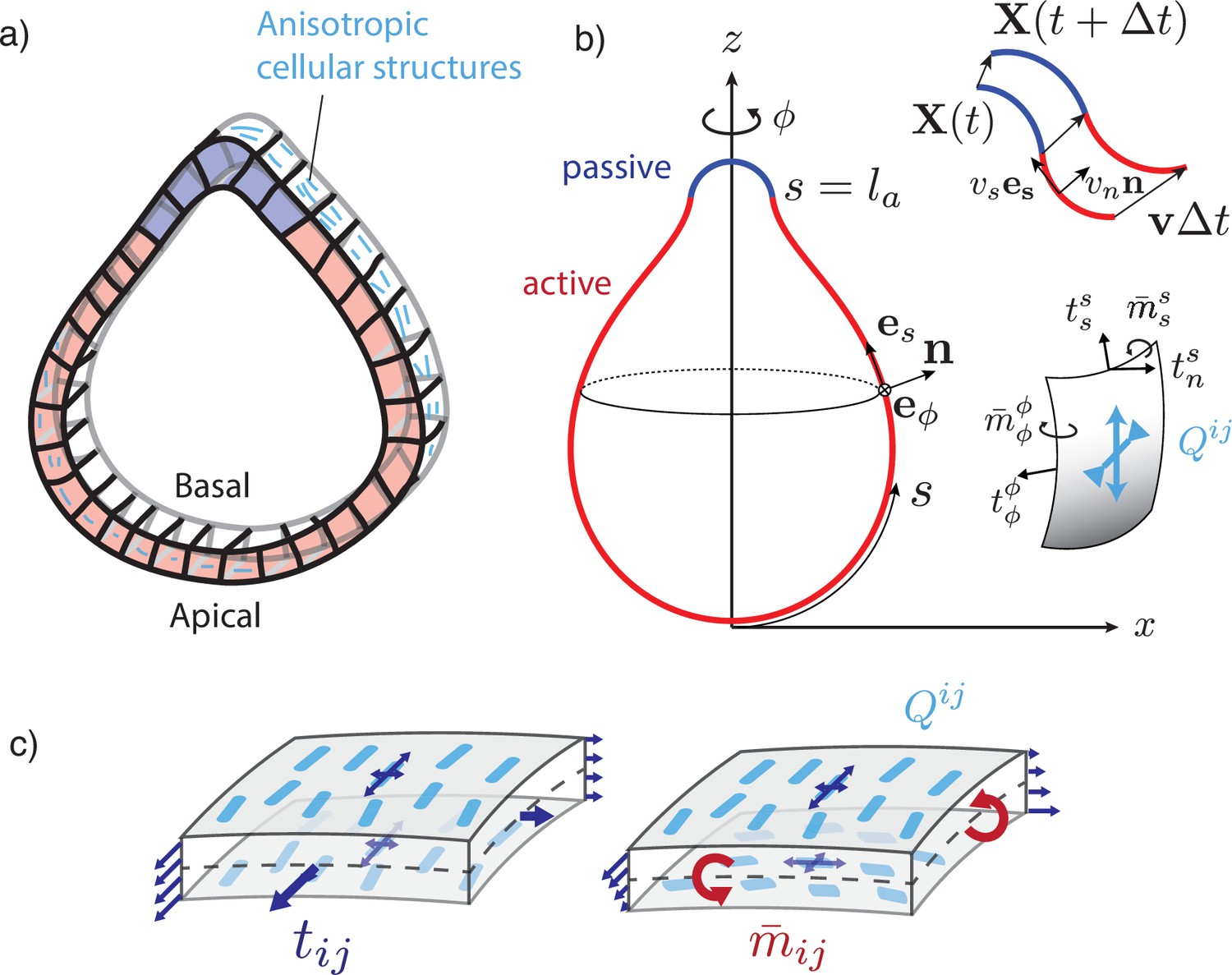
A two-dimensional surface with nematic order represents an epithelial sheet undergoing active deformations.
(a) Schematic of an epithelial tissue with a cellular state pattern. (b) Parametrisation of the axially symmetric shell and its deformation with the flow , and components of the tension and torque tensors. We note that and . (c) Stresses integrated across the thickness of the sheet result in tensions and bending moments acting on the midsurface. Anisotropic and possibly different tensions (dark-blue arrow crosses) on the apical and basal sides of the epithelium result in anisotropies in and , which can be captured by a nematic order parameter (e.g. blue rods on the top surface).
Figure 1—video 1
Deformation of an epithelial shell with free volume, , , with active torque colour coded.
Figure 1—video 2
Deformation of an epithelial shell with free volume, , , with tangential velocity shown as white arrows and colour coded.
Figure 1—video 3
Deformation of an epithelial shell with free volume, , , with active torque colour coded.
Figure 1—video 4
Deformation of an epithelial shell with free volume, , , with tangential velocity shown as white arrows and colour coded.
Figure 1—video 5
Deformation of an epithelial shell with conserved volume, , , with active torque colour coded.
Figure 1—video 6
Deformation of an epithelial shell with conserved volume, , , with tangential velocity shown as white arrows and colour coded.
Figure 1—video 7
Deformation of an epithelial shell with conserved volume, , , with active torque colour coded.
Figure 1—video 8
Deformation of an epithelial shell with conserved volume, , , with tangential velocity shown as white arrows and colour coded.
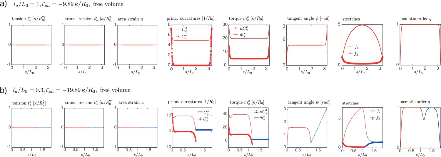
Figure 2 with 10 supplements
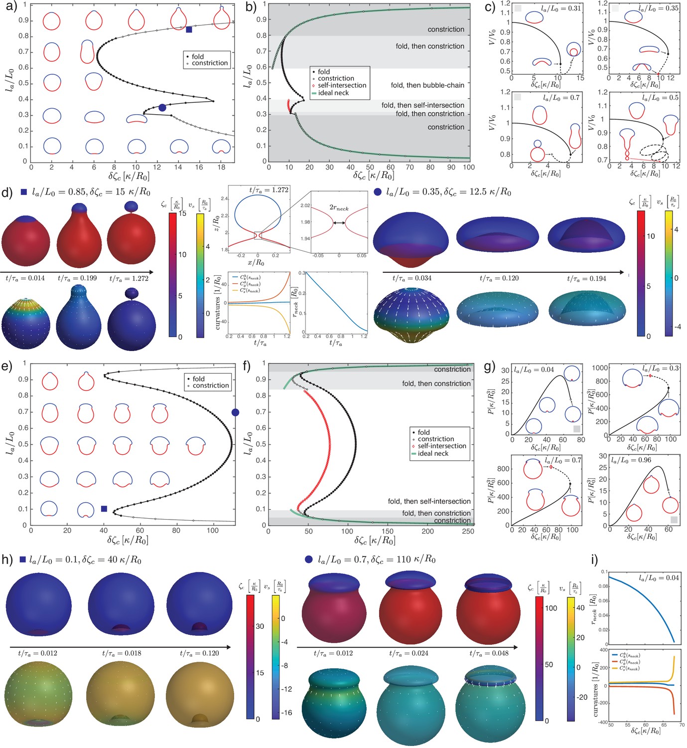
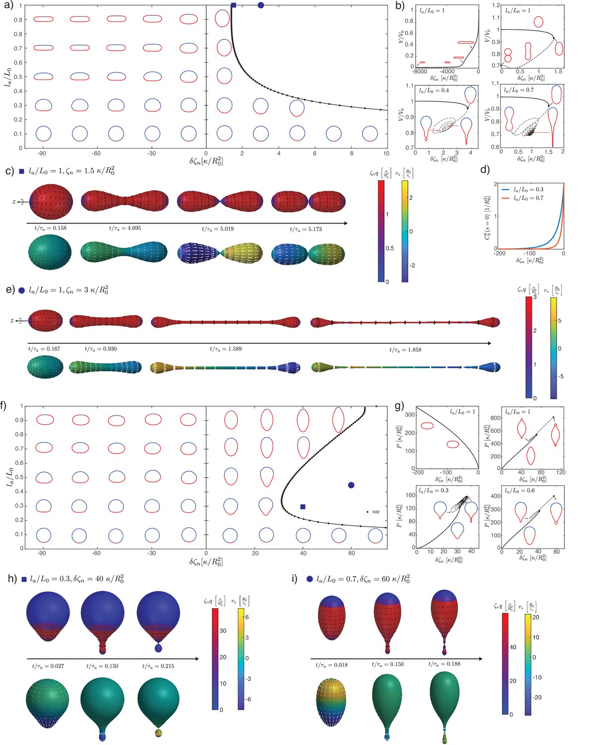
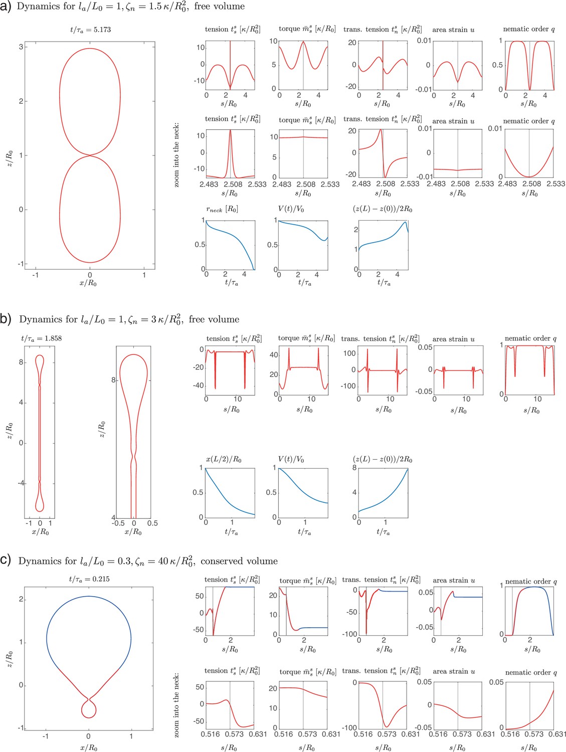
Deformations of epithelial shells due to active bending moments, with free (a–d) and conserved (e–i) volume.
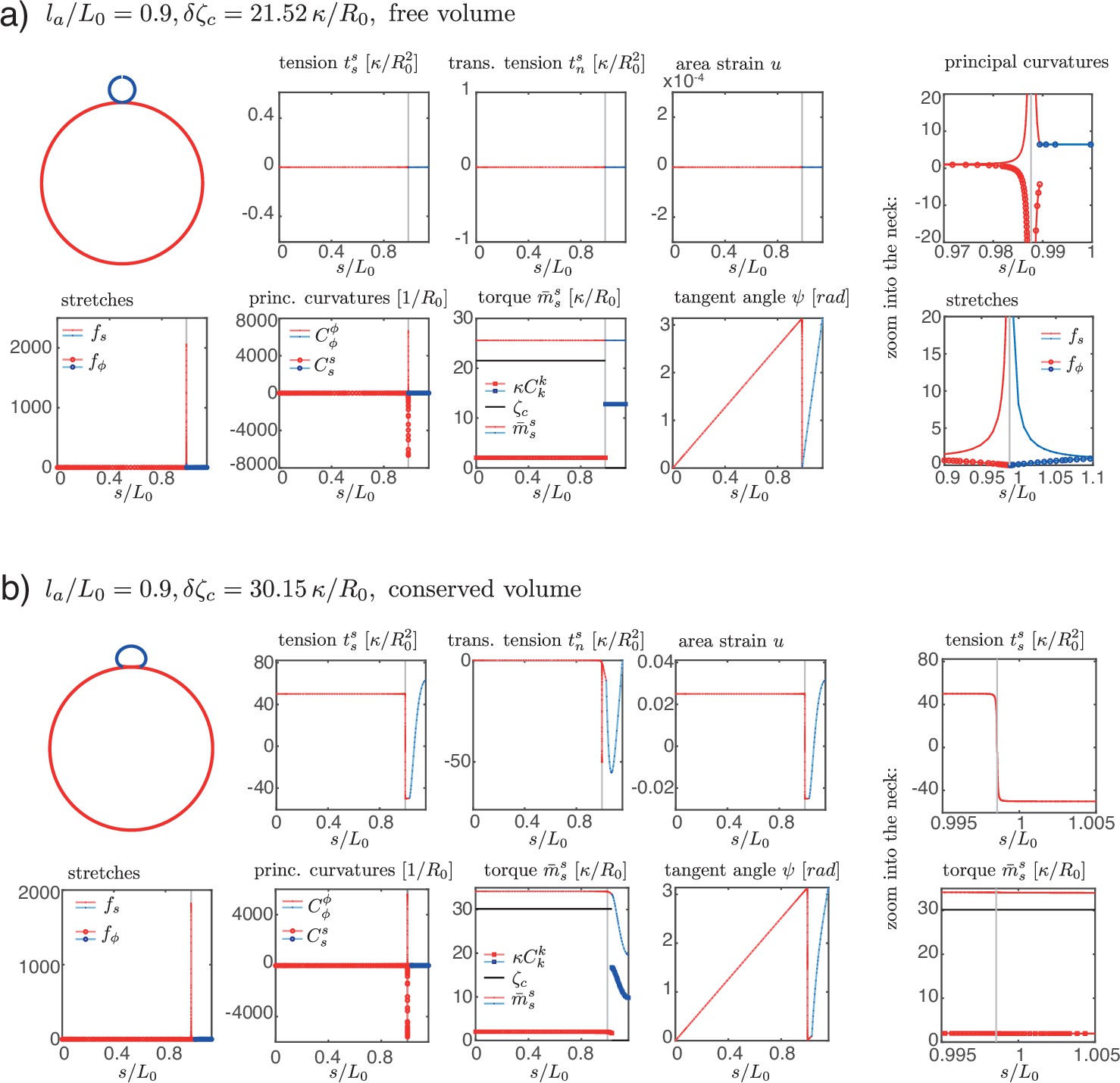
(a, e) Shape diagram. (b, f) Details of shape diagram illustrating different behaviours of solution branches. The ideal neck line (green) represents the bending moment difference required to create budded shapes consisting of two spheres with , as given by Equation 24. (c) Examples of solution branches in the -plane corresponding to four different regions in (b). (g) Examples of solution branches in the -plane chosen from three different regions in (e). (d, h) Dynamic simulations of shape changes, for parameter values indicated in the shape diagrams (a, e). (i) Neck radius and curvatures at the neck as functions of for the example in (g). Other parameters: , .
Figure 2—figure supplement 1
Details of the steady-state solutions with nearly closed necks formed by isotropic bending moments for free volume (a) and conserved volume (b), and .
The location of the neck, taken as the point where is maximal, is marked by a grey line in the plots. (a) The shape is characterised by and constant.. (b) Here, changes sign and is continuous across the neck.
Figure 2—figure supplement 2
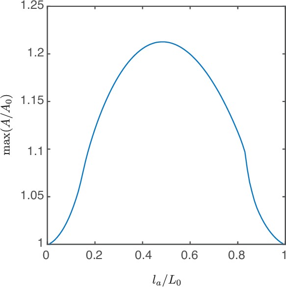
Maximal relative surface area of the steady-state shapes measured along a solution branch for each in the case of conserved volume, corresponding to shapes shown in Figure 2e–g.
Figure 2—video 1
Deformation of an epithelial shell with free volume, , , with nematic director shown with black lines and active nematic tension colour coded.
Figure 2—video 2
Deformation of an epithelial shell with free volume, , , with tangential velocity shown as white arrows and colour coded.
Figure 2—video 3
Deformation of an epithelial shell with free volume, , , with nematic director shown with black lines and active nematic tension colour coded.
Figure 2—video 4
Deformation of an epithelial shell with free volume, , , with tangential velocity shown as white arrows and colour coded.
Figure 2—video 5
Deformation of an epithelial shell with conserved volume, , , with nematic director shown with black lines (where ) and active nematic tension colour coded.
Figure 2—video 6
Deformation of an epithelial shell with conserved volume, , , with tangential velocity shown as white arrows and colour coded.
Figure 2—video 7
Deformation of an epithelial shell with conserved volume, , , with nematic director shown with black lines (where ) and active nematic tension colour coded.
Figure 2—video 8
Deformation of an epithelial shell with conserved volume, , , with tangential velocity shown as white arrows and colour coded.
Figure 3
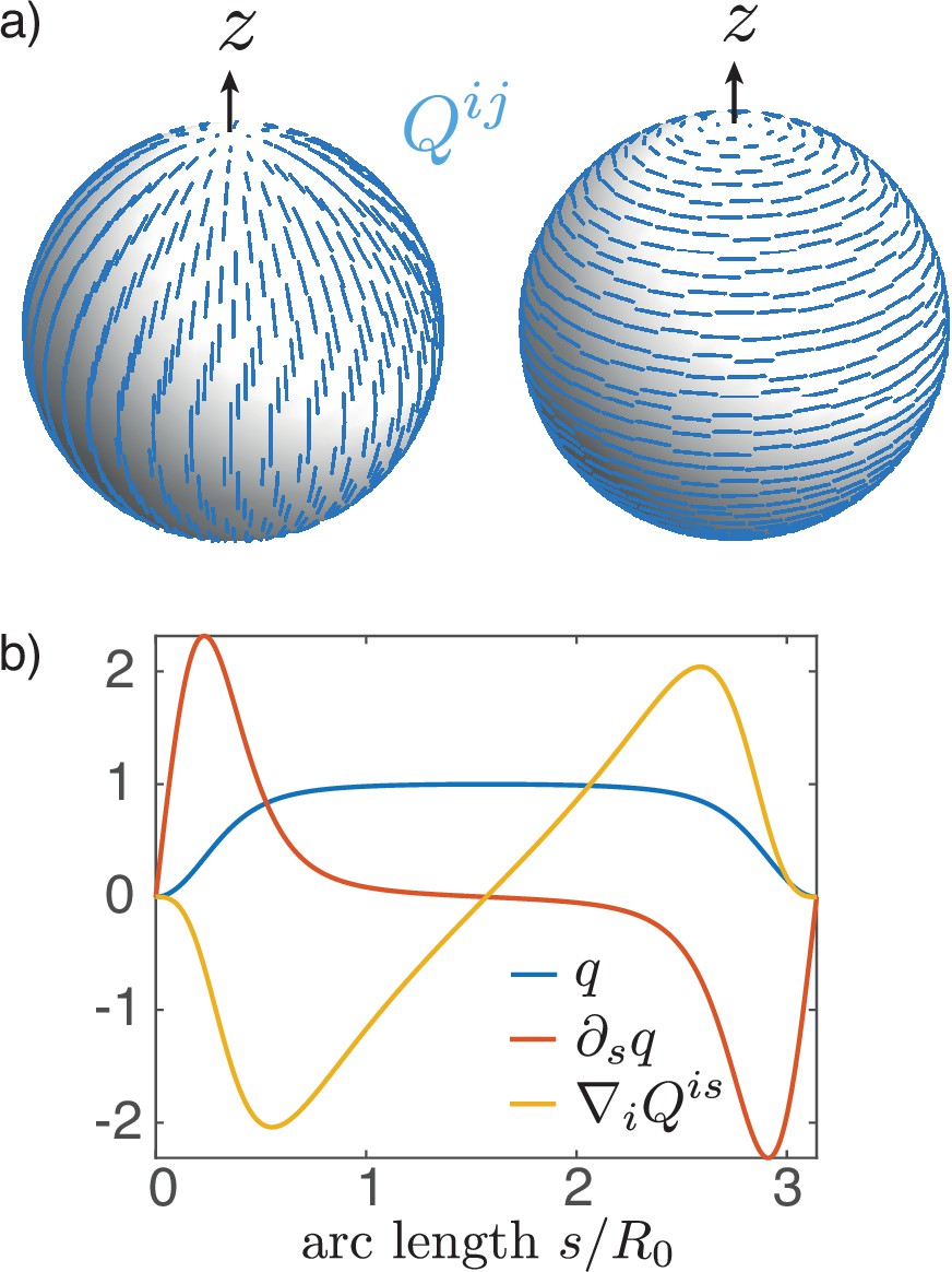
Nematic order on a sphere.
(a) Two possible configurations for the nematic order parameter on a sphere with a + 1 topological defect at each pole: meridional (left) or circumferential (right) alignment. The order parameter minimises an effective energy (Equation 9 with ). (b) Order parameter as a solution of the Euler–Lagrange Equation 16 on a sphere with and at the equator and at the locations of the defects (poles). For uniform , is the active nematic contribution to the tangential force balance (Equation 63) and, close to the equator, results in the elongation of the surface along the axis of symmetry for , and its contraction for .
Figure 4 with 13 supplements
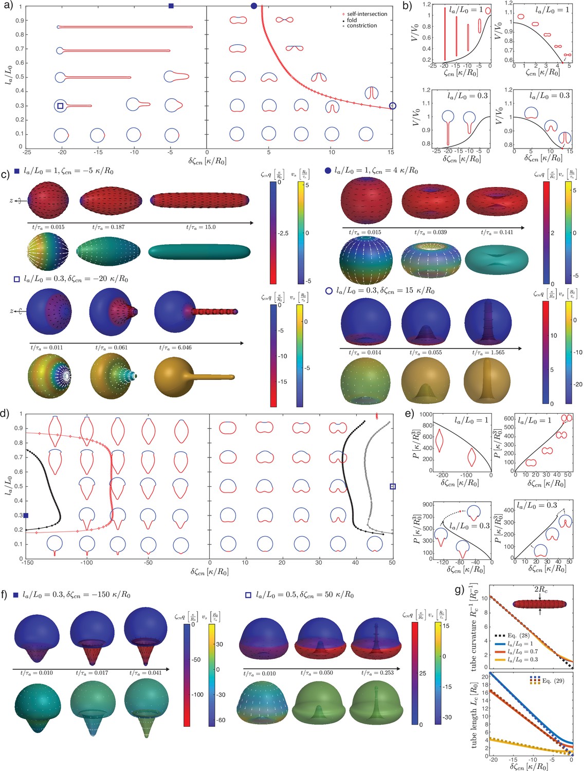
Deformations of epithelial shells due to nematic tensions, with free (a–e) and conserved (f–i) volume.
(a, e) Shape diagrams. (b, g) Details of shape diagram illustrating the behaviour of solution branches. (d) Curvature at the south pole for extensile stress. (c, e, h, i) Dynamic simulations of shell shape changes, for parameter values indicated in the phase diagrams (a, f). Other parameters: , , .
Figure 4—figure supplement 1
Details of dynamics simulations for shells with (a, b) homogeneous and (c) patterned nematic tension, which result in one or two constricting necks.
Surface quantities are shown for the last plotted time step in Figure 4. The location of the neck, taken as the point where is maximal, is marked by a grey line in the plots. In (a, b) the radius at the equator, the volume, and the pole–pole distance are shown as functions of time. In (c) the smooth sigmoidal pattern of is visualised as two discrete regions (colour coded as red and blue) for simplicity. The parameter values correspond to the examples in Figure 4c, e and h in the main text.
Figure 4—video 1
Deformation of an epithelial shell with free volume, , , with nematic director (black lines, as described in figure caption) and active nematic torque colour coded.
Figure 4—video 2
Deformation of an epithelial shell with free volume, , , with tangential velocity shown as white arrows and colour coded.
Figure 4—video 3
Deformation of an epithelial shell with free volume, , , with nematic director (black lines, as described in figure caption) and active nematic torque colour coded.
Figure 4—video 4
Deformation of an epithelial shell with free volume, , , with tangential velocity shown as white arrows and colour coded.
Figure 4—video 5
Deformation of an epithelial shell with free volume, , , with nematic director (black lines, as described in figure caption) and active nematic torque colour coded.
Figure 4—video 6
Deformation of an epithelial shell with free volume, , , with tangential velocity shown as white arrows and colour coded.
Figure 4—video 7
Deformation of an epithelial shell with free volume, , , with nematic director (black lines, as described in figure caption) and active nematic torque colour coded.
Figure 4—video 8
Deformation of an epithelial shell with free volume, , , with tangential velocity shown as white arrows and colour coded.
Figure 4—video 9
Deformation of an epithelial shell with conserved volume, , , with nematic director (black lines, as described in figure caption) and active nematic torque colour coded.
Figure 4—video 10
Deformation of an epithelial shell with conserved volume, , , with tangential velocity shown as white arrows and colour coded.
Figure 4—video 11
Deformation of an epithelial shell with conserved volume, , , with nematic director (black lines, as described in figure caption) and active nematic torque colour coded.
Figure 4—video 12
Deformation of an epithelial shell with conserved volume, , , with tangential velocity shown as white arrows and colour coded.
Figure 5 with 1 supplement
Deformations of epithelial shells due to nematic bending moments, with free (a–c) and conserved (d, e) volume.
(a, d) Shape diagrams. (b, e) Details of shape diagram illustrating the behaviour of solution branches. (c, f) Dynamic simulations of shell shape changes, for parameter values indicated in the phase diagrams (a, d). In both cases in (f) the dynamics results in self-intersection. (g) Comparison of curvature and length of the cylindrical tubes for , with analytical predictions. The tube length is measured on the steady-state shape as the arc length of the deformed active region, , and the tube curvature as . Other parameters: , , . In (c), (f), for the orientation of the director field drawn on the surface (black lines) is set by .
Figure 5—figure supplement 1
Details of steady-state shapes resulting from nematic bending moments with and free volume.
(a) Closed cylinder; (b) shape with cylindrical appendage. Such solutions are characterised by everywhere, and a cylindrical part where and is constant.
Figure 6
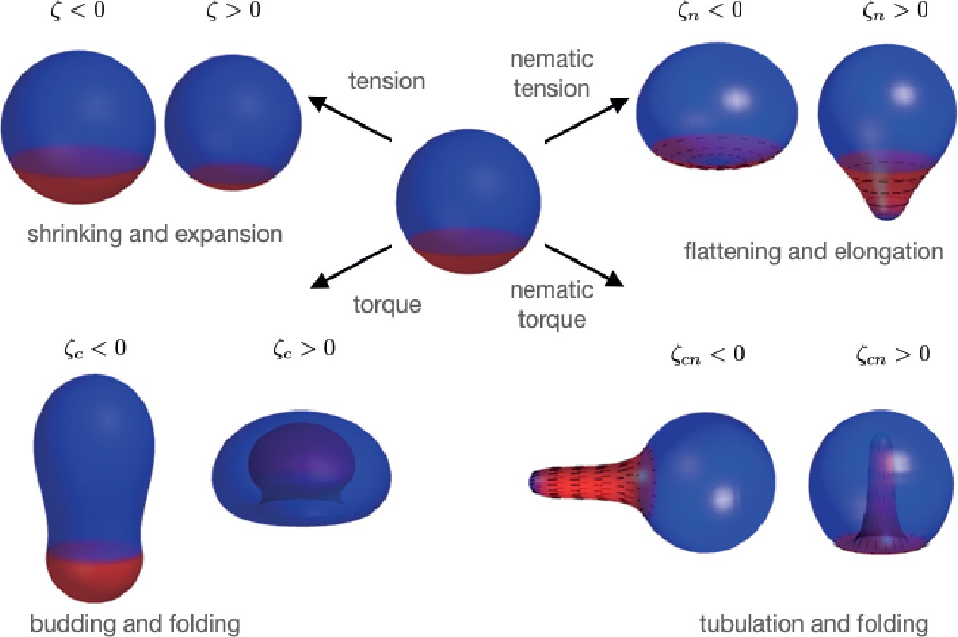
Summary of shape changes obtained through patterning of isotropic and anisotropic active tensions and bending moments.
Active tensions and bending moments are present only in the red region of the surface. For the director field orientation (black lines) is set by .
Appendix 1—figure 1
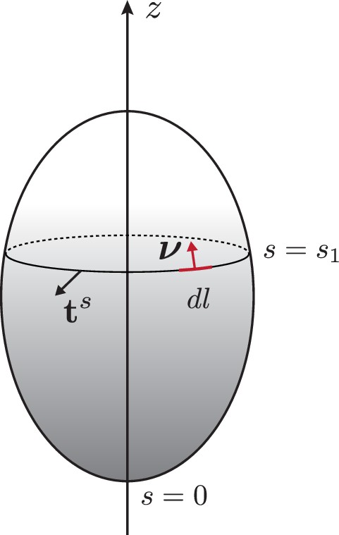
Schematic of the surface used to derive the integral of the normal force balance.
Appendix 4—figure 1
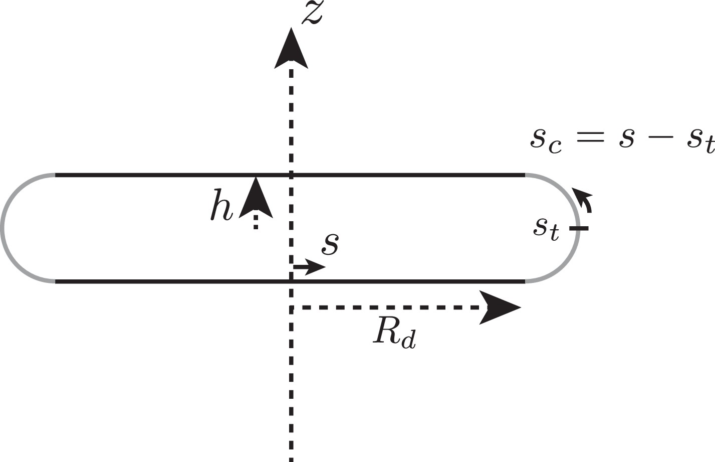
Schematic of notations used for the asymptotic analysis of a bilayered disc.
Appendix 4—figure 2
Details of shape and nematic profiles for flattened steady-state shapes resulting from a homogeneous nematic tension.
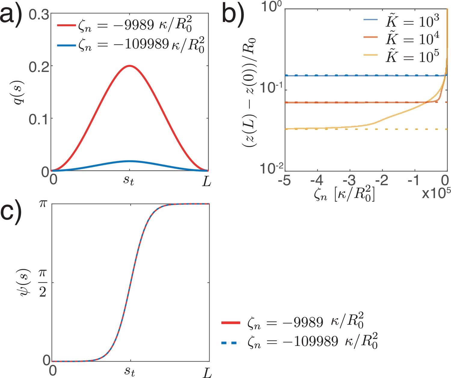
(a) Profile of nematic order parameter q, which decreases for increasing . (b) Distance between the poles of the steady-state solution for different values of and , and corresponding prediction of Equation 134 (dotted lines). (c) Profile of for different values of . The profile is invariant with respect to , for large values of .
Appendix 7—figure 1
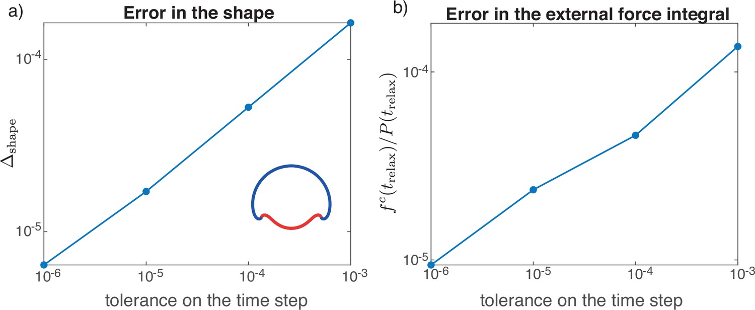
Convergence analysis of a dynamics simulation to a steady state obtained from direct calculation, for the example shape shown in the inset of (a).
For different (time step) the error in the shape in (a) and error in the external force integral in (b) are shown.
Appendix 8—figure 1

Rescaling of the size of the active region with active tension difference.
(a) Plot of as given by Equations 213; 214. This illustrates the rescaling of the active region size as a function of the tension difference , for initial values (blue to purple). (b) Shapes corresponding to two points on the curve.
Author response image 1
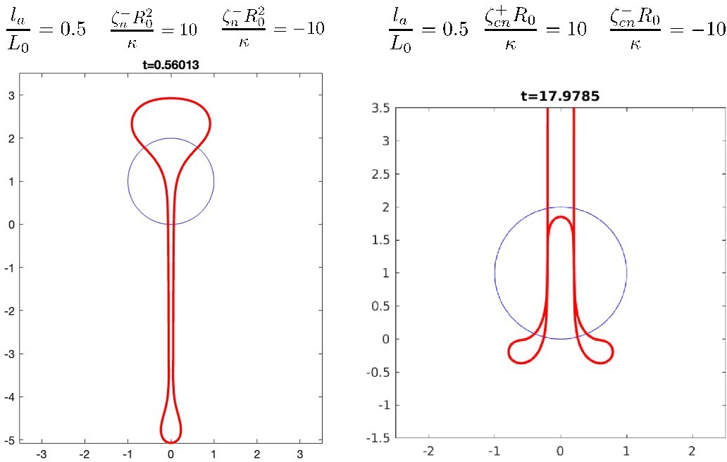
Shapes obtained with two contiguous domains of extensile and contractile nematic active tension (left) or nematic active bending moments (right).
Parameter values with + and – subscripts indicate values in the contractile and extensile regions. The contractile region is at the bottom of the shape.
Author response image 2

Results of dynamics simulations that converge to a steady state (light blue circles) overlaid with solution branches from the main text.
Since in the dynamics a smooth profile is used, rather than a step function as in the direct calculation, there is a small deviation between the two in some cases. We checked on two cases that if the smooth profile is used in the steady-state equation the match becomes excellent (b, blue dotted lines).
Additional files
Download links
A two-part list of links to download the article, or parts of the article, in various formats.
Downloads (link to download the article as PDF)
Open citations (links to open the citations from this article in various online reference manager services)
Cite this article (links to download the citations from this article in formats compatible with various reference manager tools)
Active morphogenesis of patterned epithelial shells
eLife 12:e75878.
https://doi.org/10.7554/eLife.75878


