Binary and analog variation of synapses between cortical pyramidal neurons
- Princeton Neuroscience Institute, Princeton University, United States
- Computer Science Department, Princeton University, United States
- Brain & Cognitive Sciences Department, Massachusetts Institute of Technology, United States
- Allen Institute for Brain Science, United States
- Department of Neuroscience, Baylor College of Medicine, United States
- Center for Neuroscience and Artificial Intelligence, Baylor College of Medicine, United States
- Department of Electrical and Computer Engineering, Rice University, United States
Figures
Figure 1 with 3 supplements

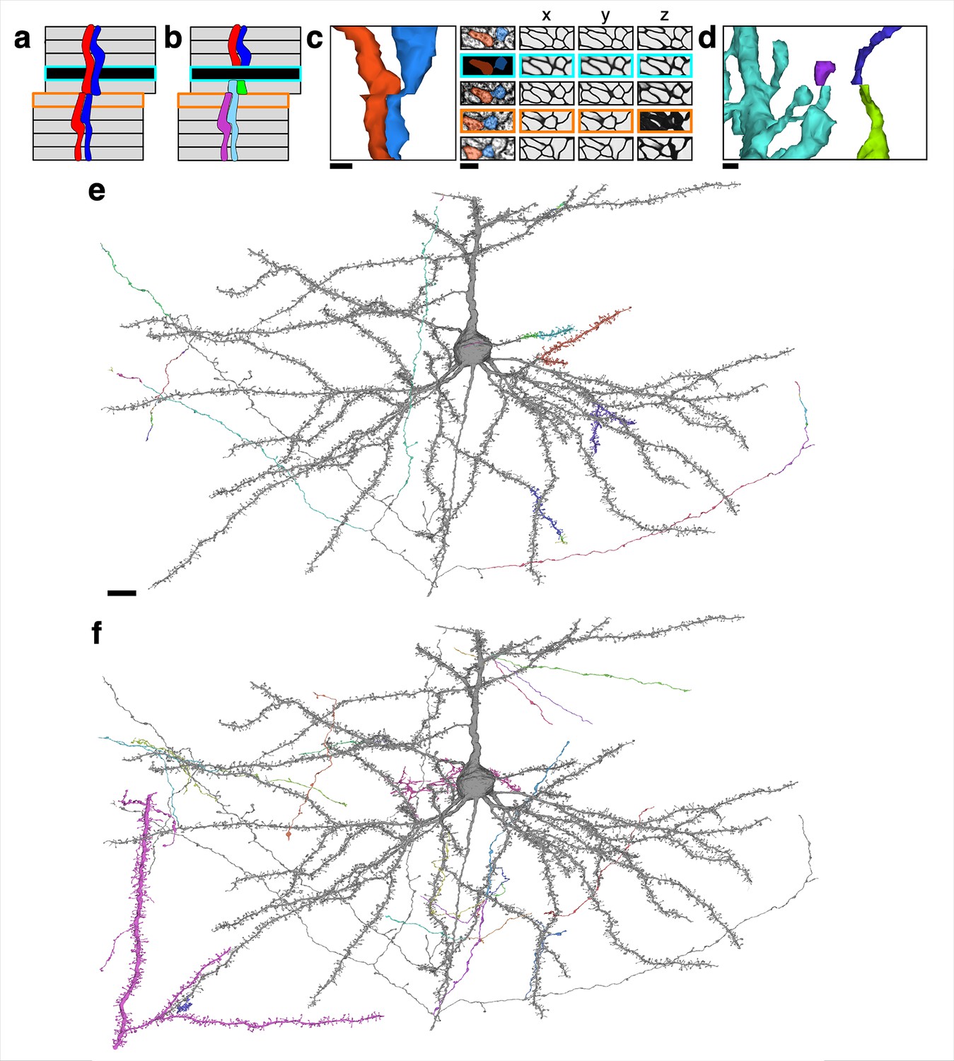
Reconstructing cortical circuits in spite of serial section electron microscopy (ssEM) image defects.
(a) Ideally, imaging serial sections followed by computational alignment would create an image stack that reflects the original state of the tissue (left). In practice, image stacks end up with missing sections (blue) and misalignments (green). Both kinds of defects are easily simulated when training a convolutional net to detect neuronal boundaries. Small subvolumes are depicted rather than the entire stack, and image defects are typically local rather than extending over an entire section. (b) The resulting net can trace more accurately, even in images not previously seen during training. Here, a series of five sections contains a missing section (blue frame) and a misalignment (green). The net ‘imagines’ the neurites through the missing section, and traces correctly in spite of the misalignment. (c) 3D reconstructions of the neurites exhibit discontinuities at the misalignment, but are correctly traced. (d) All 362 pyramidal cells with somas in the volume (gray), cut away to reveal a few examples (colors). (e) Layer 2/3 (L2/3) pyramidal cell reconstructed from ssEM images of mouse visual cortex. Scale bars: 300 nm (b).
Figure 1—figure supplement 1
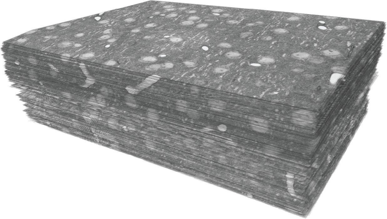
Reconstruction of connections between layer 2/3 (L2/3) pyramidal cells.
250×140×90 µm3 3D image stack from L2/3 of mouse primary visual cortex.
Figure 1—figure supplement 2
Examples of reconstructed neurites near image defects.
(a) Illustration of a possible pair of neurites that pass through both missing section (cyan) and misalignment (orange) defects. (b) Illustration of a naive segmentation of the pair in (a). (c) Same examples as in Figure 1, accompanied by affinity map. Scale bar: 300 nm. (d) Near a larger misalignment, the displacement is larger than the width of a thin neurite, and the convolutional net is unable to trace through the misalignment. Scale bar 300 nm. (e) A proofread neuron (gray) with segments merged during proofreading (colored). Scale bar: 10 μm. (f) The same proofread neuron in (e) with pieces split during proofreading (colored).
Figure 1—figure supplement 3
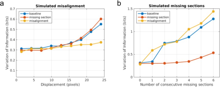
Quantitative evidence for the effectiveness of training data augmentation.
Robustness of three boundary detectors trained with no data augmentation (‘baseline’, blue), simulated missing section (‘missing section’, red), and simulated misalignment (‘misalignment’, yellow) to (a) increasingly large displacement of simulated misalignment and (b) increasing number of simulated consecutive missing sections.
Figure 2 with 2 supplements
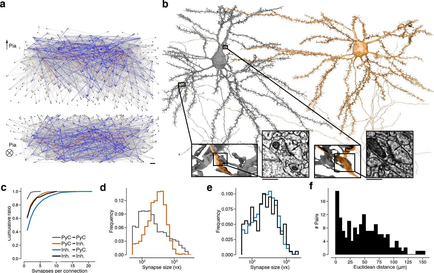
Wiring diagram for cortical neurons including multisynaptic connections.
(a) Wiring diagram of 362 proofread layer 2/3 (L2/3) pyramidal cells (PyCs) as a directed graph. Two orthogonal views with nodes at 3D locations of cell bodies. Single (gray), dual (blue), and triple, quadruple, quintuple (red) connections. (b) Dual connection from a presynaptic cell (orange) to a postsynaptic cell (gray). Ultrastructure of both synapses can be seen in closeups from the electron microscopy (EM) images. The Euclidean distance between the synapses is 64.3 μm. (c) Normalized distributions of synapses sizes for L2/3 PyCs synapses separated by postsynaptic cell type. (d) Same as (c) for inhibitory cells in layer 2/3. (e) Cumulative distributions of the number of synapses per connection for different pre- and postsynaptic cell types. (f) Distribution of Euclidean distances between synapse pairs of dual connections. Median distance is 46.5 μm. Scale bars: 10 μm (a), 500 nm (b).
Figure 2—figure supplement 1
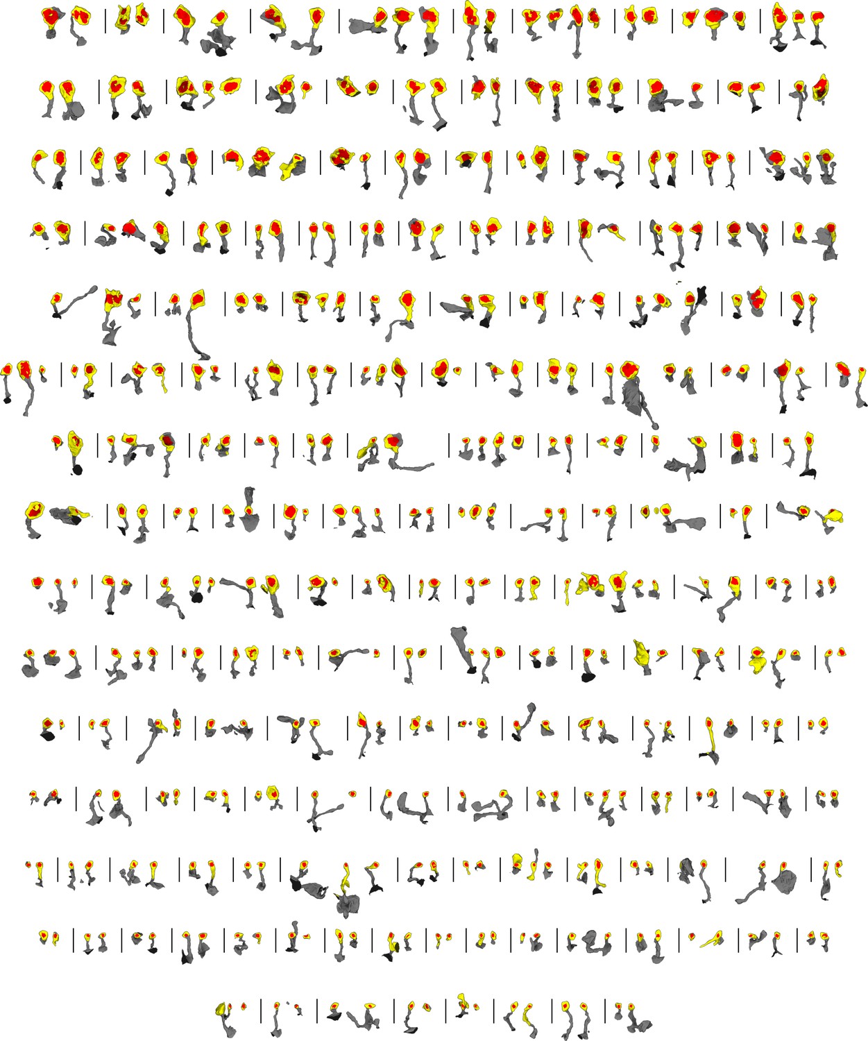
Renderings of all synapses from multisynaptic connections between layer 2/3 (L2/3) pyramidal cells.
Dendritic spines (yellow) and synaptic clefts (red) are rendered in 3D. Most are dual connections (160), but there are also triples (24), quadruples (3), and quintuples (2).
Figure 2—figure supplement 2
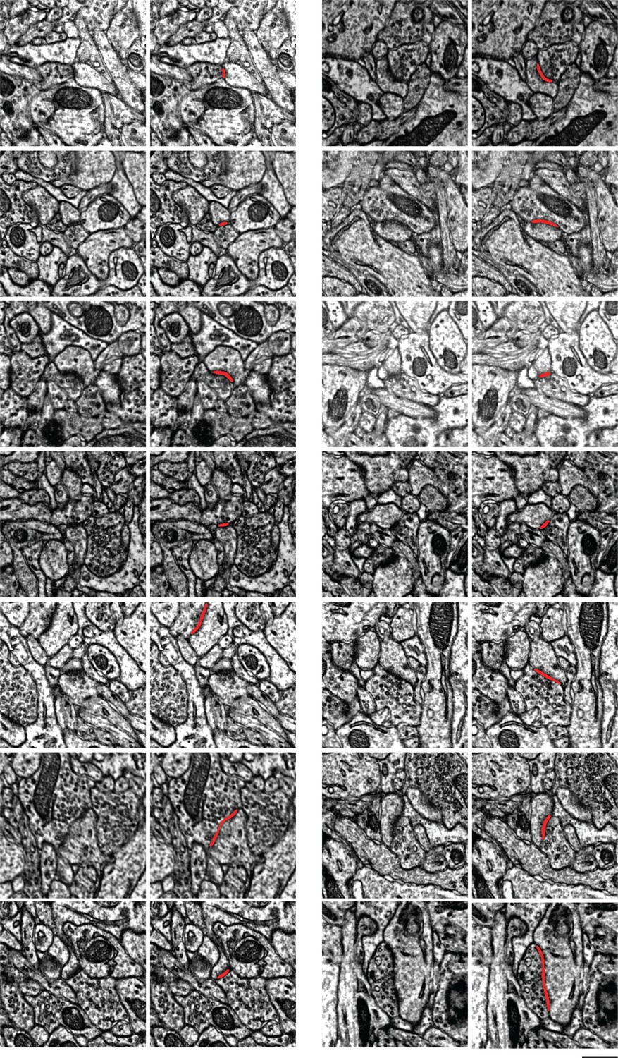
Examples of synapses between layer 2/3 (L2/3) pyramidal cells.
Scale bar: 500nm. In each pair of images, the left shows one section through a synapse, and the right adds the automatically detected cleft as an overlay. Note here that the clefts are associated with postsynaptic densities.
Figure 3 with 7 supplements
Modeling spine head volume with a mixture of two log-normal distributions.
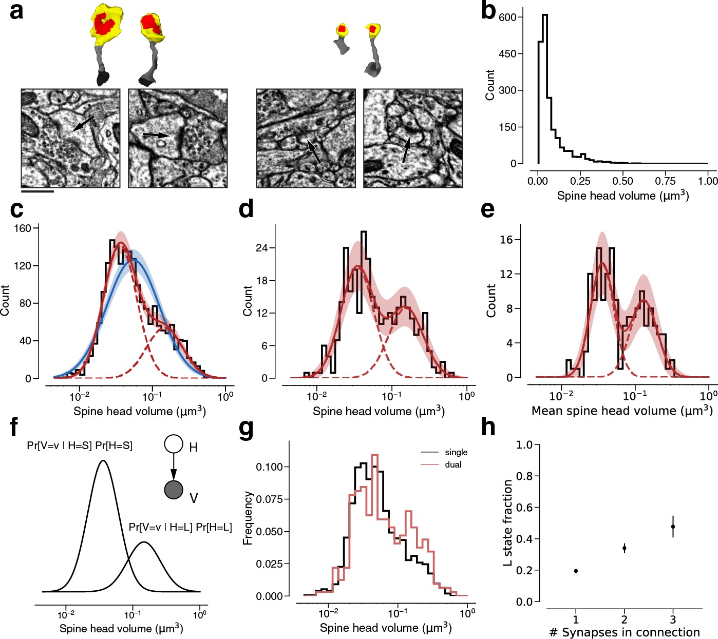
(a) Dendritic spine heads (yellow) and clefts (red) of dual connections between layer 2/3 pyramidal cells (L2/3) PyCs. The associated electron microscopy (EM) cutout shows a 2D slice through the synapse. The synapses are centered in the EM images. (b) Skewed histogram of spine volume for all 1960 recurrent synapses between L2/3 PyCs, with a long tail of large spines. (c) Histogram of the spine volumes in (b), logarithmic scale. A mixture (red, solid) of two log-normal distributions (red, dashed) fits better (likelihood ratio test, p<1e-39, n=1960) than a single normal (blue). (d) Spine volumes belonging to dual connections between L2/3 PyCs, modeled by a mixture (red, solid) of two log-normal distributions (red, dashed). (e) Dual connections between L2/3 PyCs, each summarized by the geometric mean of two spine volumes, modeled by a mixture (red, solid) of two log-normal distributions (red, dashed). (f) Mixture of two normal distributions as a probabilistic latent variable model. Each synapse is described by a latent state H that takes on values ‘S’ and ‘L’ according to the toss of a biased coin. Spine volume V is drawn from a log-normal distribution with mean and variance determined by latent state. The curves shown here represent the best fit to the data in (d). Heights are scaled by the probability distribution of the biased coin, known as the mixture weights. (g) Comparison of spine volumes for single (black) and dual (red) connections. (h) Probability of the ‘L’ state (mixture weight) versus number of synapses in the connection. Error bars are standard deviations estimated by bootstrap sampling. Scale bar: 500nm (a). Error bars are of the model fit (c, d, e) and standard deviation from bootstrapping (h).
Figure 3—figure supplement 1
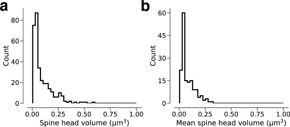
Linear spine head volume distributions.
(a) Spine volumes belonging to dual connections between layer 2/3 pyramidal cells (L2/3 PyCs). (b) Dual connections between L2/3 PyCs, each summarized by the geometric mean of two spine volumes.
Figure 3—figure supplement 2
Arithmetic means.
(a) Dual connections between layer 2/3 pyramidal cells (L2/3 PyCs), each summarized by the arithmetic mean of two spine volumes, modeled by a mixture (red, solid) of two normal distributions (red, dashed). (b) Dual connections between L2/3 PyCs, each summarized by the arithmetic mean of two cleft sizes, modeled by a mixture (red, solid) of two normal distributions (red, dashed). Error bars are of the model fit.
Figure 3—figure supplement 3

Fits versus raw data histograms.
Plots are analogous to Figure 3 and Figure 3—figure supplement 2. (a) Histogram of same spine volumes, logarithmic scale. A mixture (red, solid) of two log-normal distributions (red, dashed) is shown. (b) Spine volumes belonging to dual connections between layer 2/3 pyramidal cells (L2/3 PyCs), modeled by a mixture (red, solid) of two log-normal distributions (red, dashed). (c) Dual connections between L2/3 PyCs, each summarized by the geometric mean of two spine volumes, modeled by a mixture (red, solid) of two log-normal distributions (red, dashed). (d) Dual connections between L2/3 PyCs, each summarized by the arithmetic mean of two spine volumes, modeled by a mixture (red, solid) of two log-normal distributions (red, dashed).
Figure 3—figure supplement 4
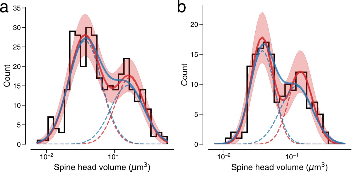
Modeling spine volume with a bimodal versus unimodal mixture of two normal distributions.
(a) Spine volumes belonging to dual connections between layer 2/3 (L2/3) pyramidal cells. A bimodal mixture (red, solid) of two normal distributions (red, dashed) is a better fit than a unimodal mixture (blue, solid) of two normal distributions (blue, dashed) (see Holzmann and Vollmer, 2008; p=0.0425, n=320). The bimodal mixture weights are 60:40. (b) Dual connections between L2/3 pyramidal cells, each summarized by the geometric mean of spine volumes. A bimodal mixture (red, solid) of two normal distributions (red, dashed) is a better fit than a unimodal mixture (blue, solid) of two normal distributions (blue, dashed) (likelihood ratio test, p=0.0059, n=160). Error bars are of the model fit.
Figure 3—figure supplement 5
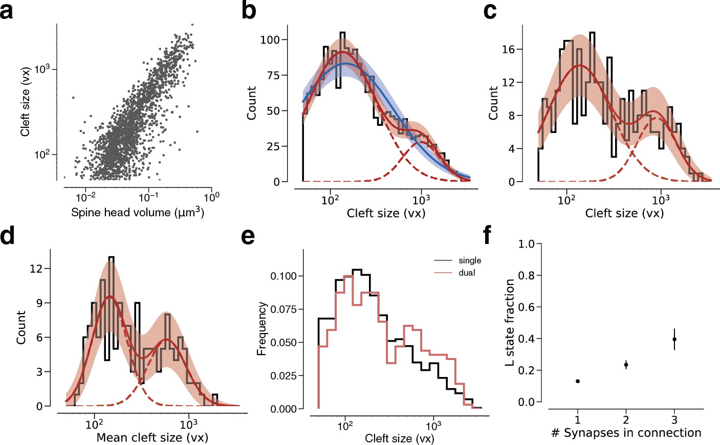
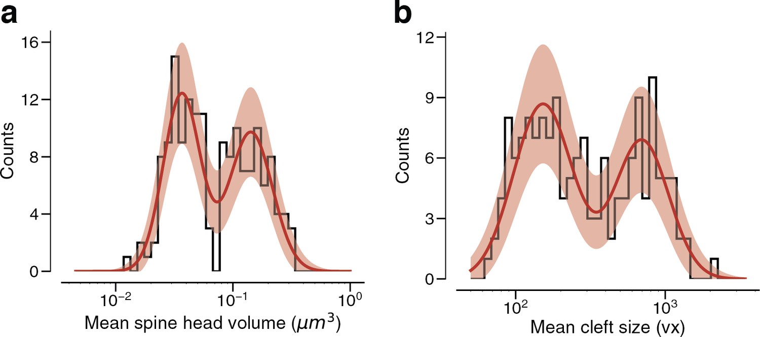
Modeling cleft size with a mixture of two normal distributions.
(a) Spine volume versus cleft size for all layer 2/3 pyramidal cell (L2/3 PyC)-L2/3 PyC synapses. (b) Histogram of same spine volumes, logarithmic scale. A mixture (red, solid) of two normal distributions (red, dashed) fits better (likelihood ratio test, p<1e-63, n=1960) than a single normal (blue). (c) Cleft sizes belonging to dual connections between L2/3 PyCs, modeled by a mixture (red, solid) of two normal distributions (red, dashed, likelihood ratio test, p=0.02, n=320). (d) Dual connections between L2/3 PyCs, each summarized by the geometric mean of two cleft sizes, modeled by a mixture (red, solid) of two normal distributions (red, dashed, likelihood ratio test, p=0.037, n=160). (e) Comparison of cleft sizes for single (black) and dual (red) connections. (f) Probability of the ‘L’ state (mixture weight) versus number of synapses in the connection. Error bars are of the model fit.
Figure 3—figure supplement 6
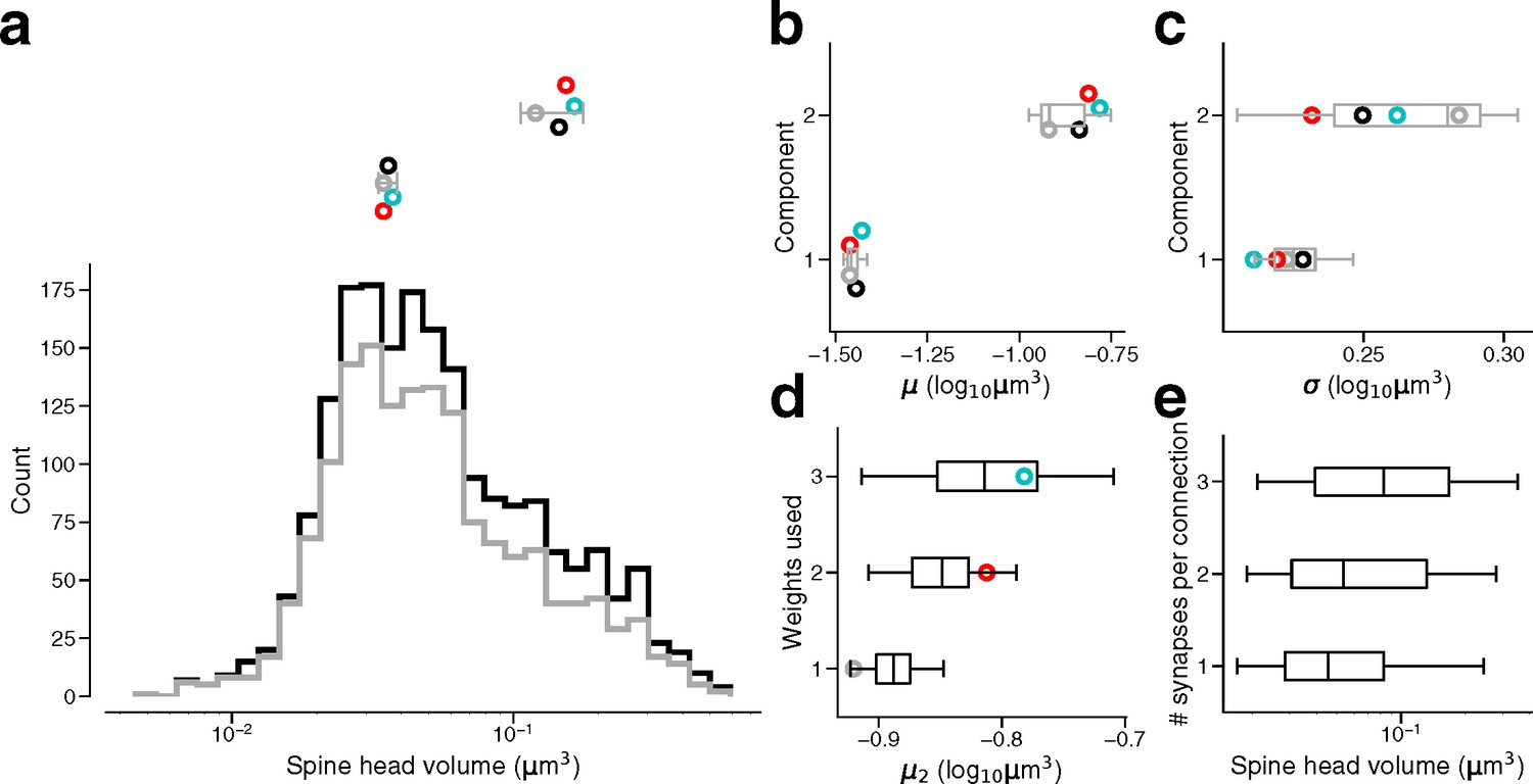
Synapse size by connection type.
(a) Bottom: Spine head volume distribution for single connections (gray) along with synapses for all connections (black). Top: parameter estimates for the component means of single connections, as well as dual connections (red), and triple connections (cyan) and all connections (black). Gray line indicates 90% bootstrap interval over the single connection synapses (1000 samples). Points jittered for clarity. (b) Parameter estimates for component means of the same populations in (a). Box indicates interquartile range across bootstrap samples. Whiskers show 90% bootstrap interval. (c) Parameter estimates for component standard deviations of the same populations in (a). (d) Second component mean estimate from GMM fits on samples of the full dataset model. Full dataset model used for sampling had component weights taken from single connection model, dual connection model, or triple connection model. Points show parameter estimate from the original GMM fit for that connection type. (e) Spine head volume by the number of synapses in a connection.
Figure 3—figure supplement 7

Relation of dendritic spine volume to spine apparatus.
(a) Examples of spine apparatus (SA) in electron microscopy (EM) images. Scale bar: 300 nm. (b) Spine volume distributions of synapses with no endoplasmic reticulum (ER) (blue), smooth ER (yellow), and SA (red). (c) Likelihood of SA (red) and ‘L’ state (black) conditioned on spine volume. (d) Spine volume distribution conditioned on SA (red) compared with size distribution conditioned on ‘L’ state (black). Inset: Joint probability distribution of SA within dual connections. Error bars are of the model fit.
Figure 4 with 6 supplements
Latent state correlations between spines at dual connections.
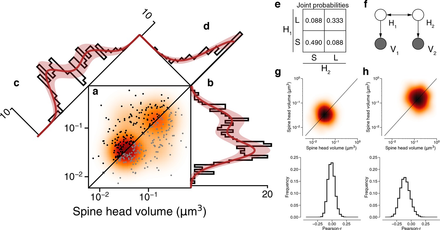
(a) Scatter plot of spine volumes (black, lexicographic ordering) for dual connections. Data points are mirrored across the diagonal (gray). The joint distribution is fit by a mixture model (orange) like that of Figure 3f, but with latent states correlated as in (e). (b) Projecting the points onto the vertical axis yields a histogram of spine volumes for dual connections (Figure 3d). Model is derived from the joint distribution. (c) Projecting onto the x=y diagonal yields a histogram of the geometric mean of spine volumes (Figure 3e). Model is derived from the joint distribution. (d) Projecting onto the x=−y diagonal yields a histogram of the ratio of spine volumes. (e) The latent states of synapses in a dual connection (H1 and H2) are more likely to be the same (SS or LL) than different (SL/LS), as shown by the joint probability distribution. (f) When conditioned on the latent states, the spine volumes (V1 and V2) are statistically independent, as shown in this dependency diagram of the model. (g), (h) Sampling synapse pairs to SS and LL states according to their state probabilities. The top shows a kernel density estimation of multiple iterations of sampling. The bottom shows the distribution of Pearson’s r correlations across many sampling rounds (N=10,000). Error bars are of the model fit.
Figure 4—figure supplement 1
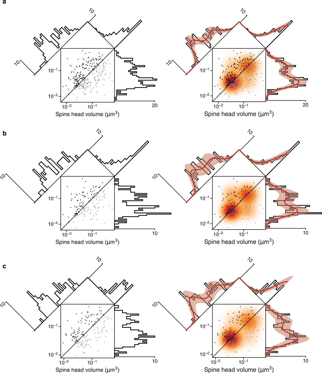
Fits versus raw distributions.
Plots are analogous to Figure 4 and Figure 4—figure supplement 4. (a) Synapse pairs from all dual connections. (b) Dual connections of synapse pairs less than the median distance apart. (c) Dual connections of synapse pairs more than the median distance apart.
Figure 4—figure supplement 2
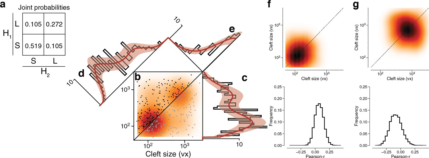
Latent state correlations between clefts at dual connections.
(a) The latent states of synapses in a dual connection are positively correlated with each other. The latent states are more likely to be the same (SS or LL) rather than different (SL or LS), as shown by the joint probability distribution. (b) Scatter plot of cleft sizes (black, lexicographic ordering) for dual connections between layer 2/3 (L2/3) pyramidal cells. Scatter plot points are mirrored across the diagonal (gray). The joint distribution is fit by a mixture model (orange) like that of Figure 3f, but with latent states that are correlated as described below. (c) Projecting the points onto the vertical axis yields a histogram of cleft sizes for dual connections, the same as in Figure 3d. Model is derived from the joint distribution. (d) Projecting the points onto the x=y diagonal yields a histogram of the geometric mean of cleft sizes for dual connections, the same as in Figure 3e. Model is derived from the joint distribution. (e) Projecting the points onto the x=−y diagonal yields a histogram of the ratio of cleft sizes for dual connections. Error bars are of the model fit.
Figure 4—figure supplement 3
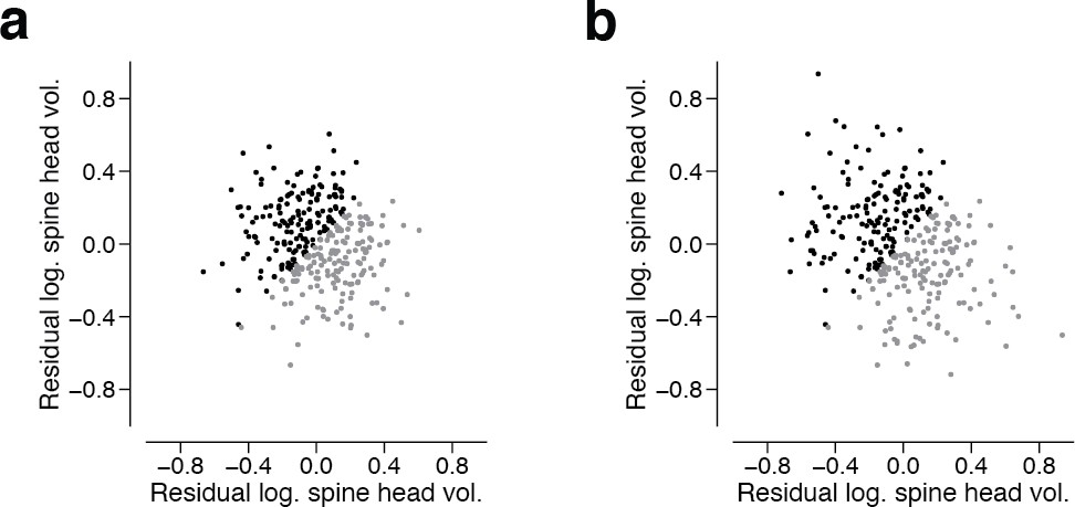
Residuals spine head volume after subtracting binary components.
We assigned the synapse pairs from the 160 dual synaptic connections to their most likely state (SS, SL, LS, LL) and subtracted the mean of the binary components. (a) shows the residual components. (b) shows the residual components when restricting assignments to SS and LL states.
Figure 4—figure supplement 4
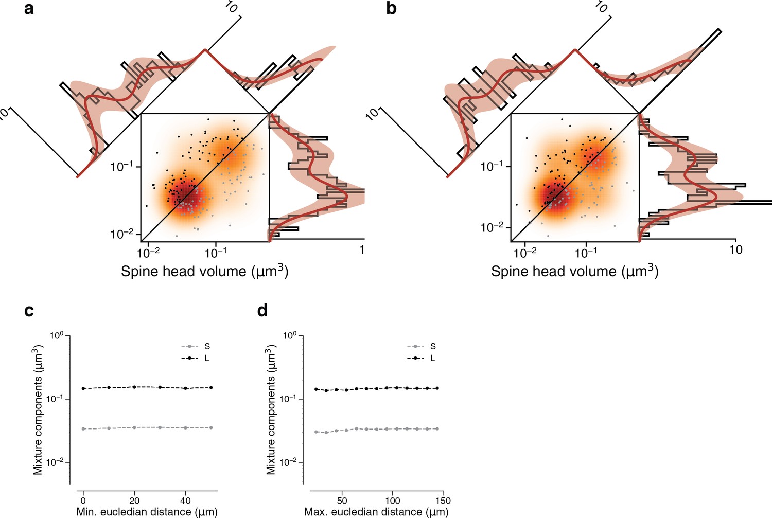
Synapses in a dual connection: near versus far pairs.
Spine volumes (left) and cleft sizes (right). (a) Dual connections of synapse pairs less than 46.5 μm apart (phi = 0.534). (b) Dual connections of synapse pairs more than 46.5 μm apart (phi = 0.745). (c) Mixture component means of model fits as a function of the minimum distance separating synapse pairs. (d) Mixture component means of model fits as a function of the maximum distance separating synapse pairs. Error bars are of the model fit.
Figure 4—figure supplement 5
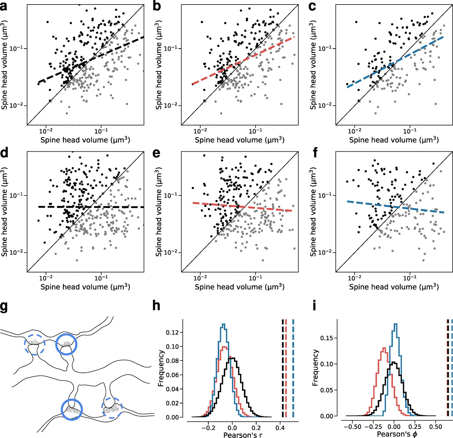
Dual connection correlations are not a result of axon or dendrite biases.
Synapses are shuffled between dual connections to measure the correlations between synapses that have the same axon (red) or the same dendrite (blue) against a fully random baseline (black). Shuffled synapses are not allowed to be paired with other synapses within their original connection. Each shuffling procedure was performed on a subset of data where at least one valid shuffling exists for each synapse (e.g. where each dendrite receives at least two dual connections). (a–c) Joint distributions of spine head volumes in the dual connections used for shuffling. Slope of linear fit shows Pearson’s r value. (a) Subset of data used for random shuffling (all 160 synapse pairs). r=0.42. (b) Subset of data used for axon-preserved shuffling (141 pairs). r=0.45. (c) Subset of data used for dendrite-preserved shuffling (89 pairs). r=0.51. (d) Example shuffle of data in (a). r=0.00. (e) Example shuffle of data in (b). r=–0.08. (f) Example shuffle of data in (c). r=–0.11. (g) Diagram of a possible shuffle of two dual synaptic connections onto the same dendrite. (h) Distribution of Pearson’s r correlation for paired spine head volumes after shuffling (100,000 shuffles each). Dashed lines indicate correlation value for the unshuffled subset. (i) Distribution of Pearson’s phi correlation for paired spine head volumes after shuffling.
Figure 4—figure supplement 6
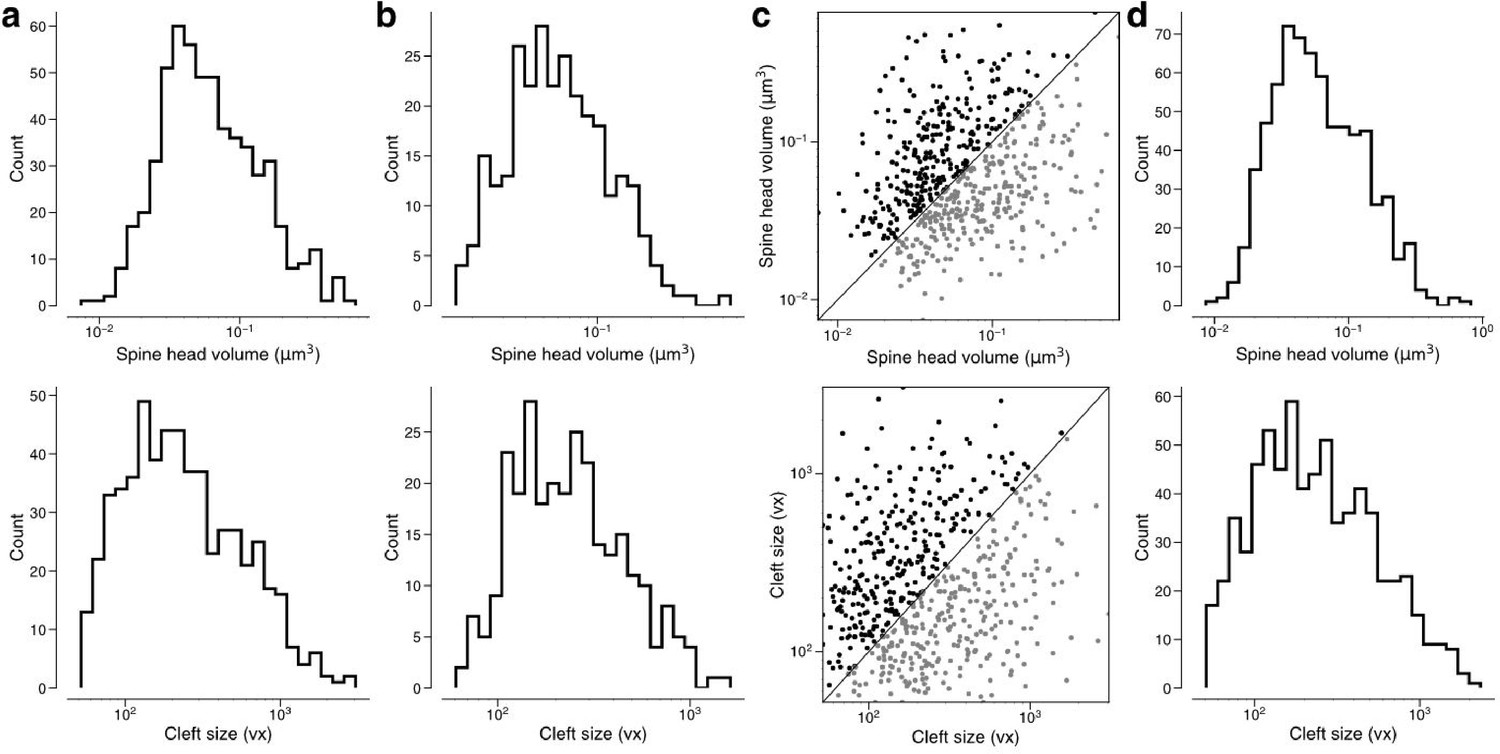
Removing constraints on the synaptic population eliminates bimodality and reduces correlations.
Spine volumes (top) and cleft sizes (bottom). (a) Distribution of synapse sizes in dual connections received by layer 2/3 (L2/3) pyramidal cells, including those from orphan axons (566 synapses). (b) Distribution of geometric means of synapse sizes in same dual connections as in (a) (283 pairs). (c) Joint distribution of synapse sizes in dual connections received by L2/3 pyramidal cells, including those from orphan axons (283 pairs). (d) Distribution of synapse sizes for excitatory synapses received by L2/3 pyramidal cells, including those from orphan axons (700 synapses).
Tables
Table 1
Overview of number of data points obtained in this study.
| Number of L2/3 PyCs in dataset | 417 |
| Number of L2/3 PyCs selected for proofreading | 362 |
| Number of proofread L2/3 PyCs connecting to any other L2/3 PyCs | 334 |
| Number of inhibitory cells in dataset | 34 |
| Number of synapses (automated) in the dataset | 3,239,275 |
| Number of outgoing synapses (automated) in the dataset from proofread L2/3 PyCs | 10,788 |
| Number of synapses between L2/3 PyCs | 1960 |
| Number of connections between L2/3 PyCs | 1735 |
| Number of connections between L2/3 PyCs with one synapse | 1546 |
| Number of connections between L2/3 PyCs with two synapses | 160 |
| Number of connections between L2/3 PyCs with three synapses | 24 |
| Number of connections between L2/3 PyCs with four synapses | 3 |
| Number of connections between L2/3 PyCs with five synapses | 2 |
Table 2
Overview of results from log-normal mixture fits for different synapse subpopulations.
| Subset of L2/3 L2/3 PyC synapses | S | L | N | ||||
|---|---|---|---|---|---|---|---|
| Mean(log10 µm3) | Std(log10 µm3) | Weight | Mean (log10 µm3) | Std(log10 µm3) | Weight | ||
| All synapses | –1.42 | 0.24 | 0.77 | –0.77 | 0.22 | 0.23 | 1960 |
| Single synapses | –1.41 | 0.24 | 0.81 | –0.76 | 0.21 | 0.19 | 1546 |
| Dual synapses | –1.44 | 0.23 | 0.64 | –0.77 | 0.21 | 0.36 | 320 |
| Triple synapses | –1.49 | 0.17 | 0.36 | –0.86 | 0.30 | 0.64 | 72 |
| All synapses with weights refitted to single synapses | (–1.42) | (0.24) | 0.80 | (–0.77) | (0.248) | 0.20 | 1960 and 1546 |
| All synapses with weights refitted to dual synapses | (–1.42) | (0.24) | 0.66 | (–0.77) | (0.248) | 0.34 | 1960 and 320 |
| All synapses with weights refitted to triple synapses | (–1.42) | (0.24) | 0.52 | (–0.77) | (0.248) | 0.48 | 1960 and 72 |
| Geometric mean of dual synapses | –1.44 | 0.16 | 0.58 | –0.87 | 0.18 | 0.42 | 160 |
| Arithmetic mean of dual synapses | –1.43 | 0.16 | 0.53 | –0.85 | 0.18 | 0.47 | 160 |
Table 3
Overview of results from hidden Markov model (HMM) log-normal component fits for different dual synaptic connection subpopulations.
| Subset of L2/3 L2/3 PyC dual synaptic connections | S | L | Weights | Pearson’s phi | N | ||||
|---|---|---|---|---|---|---|---|---|---|
| Mean(log10 µm3) | Std(log10 µm3) | Mean (log10 µm3) | Std(log10 µm3) | SS | SL+LS | LL | |||
| All connections | –1.470 | 0.216 | –0.833 | 0.244 | 0.490 | 0.177 | 0.333 | 0.637 | 160 |
| Dist <median dist | –1.506 | 0.212 | –0.861 | 0.243 | 0.427 | 0.232 | 0.342 | 0.534 | 80 |
| Dist >median dist | –1.449 | 0.207 | –0.818 | 0.251 | 0.529 | 0.123 | 0.348 | 0.745 | 80 |
Additional files
Download links
A two-part list of links to download the article, or parts of the article, in various formats.
Downloads (link to download the article as PDF)
Open citations (links to open the citations from this article in various online reference manager services)
Cite this article (links to download the citations from this article in formats compatible with various reference manager tools)
Binary and analog variation of synapses between cortical pyramidal neurons
eLife 11:e76120.
https://doi.org/10.7554/eLife.76120


