Host-parasite coevolution promotes innovation through deformations in fitness landscapes
Figures
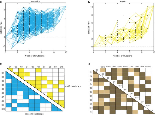
Empirical fitness landscapes of λ when infecting the (a) ancestral host and (b) malT– host, and their statistical analyses in (c) and (d).
Each node in (a) and (b) represents a unique genotype and two nodes are connected by edges if the corresponding genotypes are separated by one mutation. The node at zero mutations is ancestral λ. Selection rate (per 4 hr competition experiment) is the difference of Malthusian growth rates of a given genotype i to ancestral λ over 4 hr, calculated as , where denotes the density of the given genotype at time t. (c) Statistical analysis of direct and interactive effects of mutations in both the landscapes. Colored cells represent statistically significant terms determined by multiple regression analysis after correction for multiple hypothesis testing (see Materials and methods). The diagonal elements of the matrix represent single mutation effects and all the off-diagonal terms represent pairwise epistatic interactions. See Supplementary file 1i for identity of mutations corresponding to different . (d) Statistical test of whether the two landscapes varied in topology. The additional variable, E, represents environment (host) to indicate mutation-by-host effects in the lower-left matrix and mutation-by-mutation-by-host (G×G×E) in the upper-right matrix. Light colored cells indicate terms present in the final AIC-optimized model out of the full-factorial model (F76,726 = 37.45, p<0.0001), and dark colored cells indicate statistically significant terms after controlling for rate of false positives (see Materials and methods).
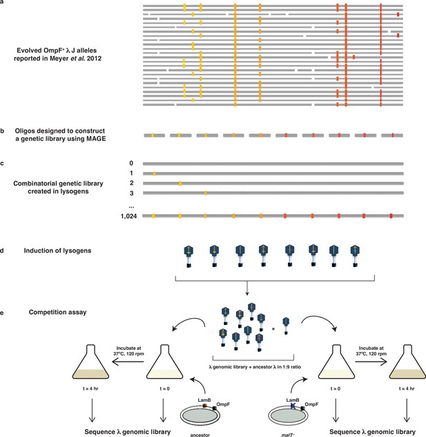
Schematic illustration of MAGE-Seq used to construct λ’s fitness landscapes.
(a) 24 independently evolved J alleles reported in Meyer et al., 2012. The white blocks indicate a location of a mutation not studied here, whereas colored blocks indicate mutations used to construct the genetic library. (b) Oligos were synthesized with focal mutations positioned in the center of the sequence. (c) MAGE was used to construct a combinatorial library of lambda lysogens integrated into E. coli’s genome. (d) Lysogens were induced in order to generate a library of λ particles with different combinations of mutations. (e) The λ library was first mixed with the ancestor in 1:9 ratio, incubated with different types of hosts for 4 hr at 37°C, and then sequenced at both initial and final timepoints to calculate the selection rates of individual genotypes.
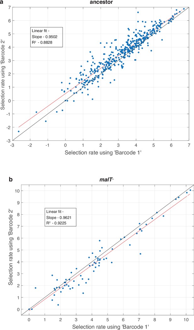
Test to determine whether amplification distorts measurements of fitness.
For every replicate population in the competition (total eight, four for each host) we performed two separate amplifications and used a unique barcode for each. This allowed us to compare fitness calculations based on independent amplifications and to determine if the amplification step is repeatable and unbiased. Each point represents a unique λ genotype presented in the fitness landscapes reported in Figure 1. The red line is a linear least-square fit. The regression fitting parameter and coefficient of determination are provided in the inset. The black line represents the vector, where fitness estimates from each barcode are equal.
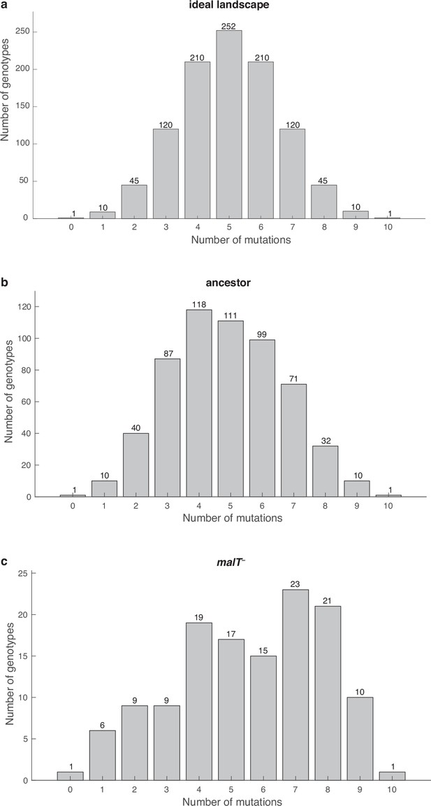
Distribution of λ genotypes present with respect to the number of mutations they possess.
(a) An ideal fitness landscape where all combinations of 10 mutations are present. (b and c) Empirical fitness landscapes with ancestral host and malT— host, respectively.
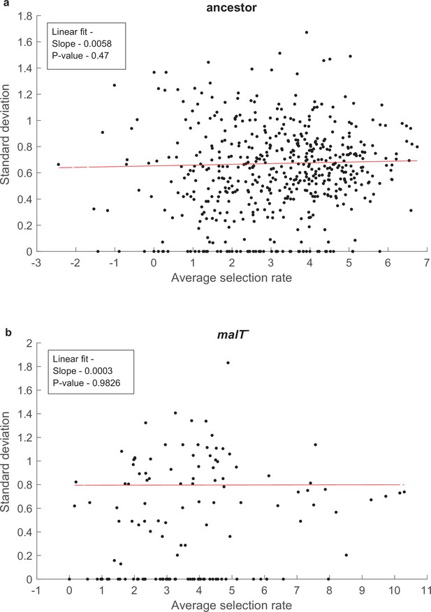
Test of whether the error in our estimates of selection rates (per 4 hr) is influenced by the magnitude of the estimate.
SD does not correlate with mean fitness of a genotypes for both (a) ancestor host, and (b) malT— host; p-values in the insets indicate that the slope is not significantly different than zero. Uniform variance in fitness values permit the performance of analysis of variance to detect genotype by genotype by host interactions. Points with zero SD indicate presence of only one replicate population with a fitness value for that genotype.
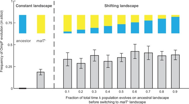
Simulation results of the frequency of OmpF-use evolution observed when fitness landscapes were shifted at different frequencies.
Each bar represents an average of 300 simulation runs. Error bars indicate 95% confidence intervals. OmpF evolution is favored when λ evolves on shifting landscapes. The only two shifting landscape treatments that are not significantly higher than simulations on the constant malT— landscape are the 0.2 and 0.4 treatments (Supplementary file 1b).
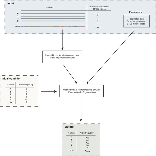
Schematic outline of the simulations used to evolve λ on the fitness landscapes.
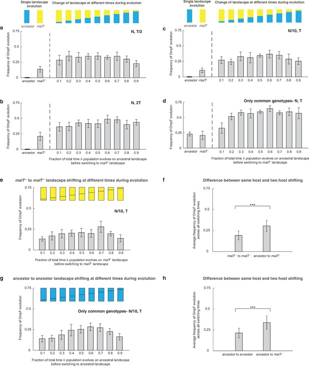
Additional simulations to verify that shifting landscapes promote OmpF+ evolution.
Frequency of OmpF+ evolution when λ population is evolved on different landscapes with different controls as compared with Figure 2 — (a) half the total number of generations, (b) twice the total number of generations, (c) with one-tenth of the population size, and (d) starting with only the genotypes whose fitness values were measured for both the landscapes. For all switching landscape treatments except two (switching fraction-time of 0.9 in (a), and 0.1 in (d)), the frequency of OmpF+ evolution was significantly higher (adjusted p-value<0.05) than the constant landscape treatments (ANOVA: F-ratio=6.62, , p<0.0001 for (a), F-ratio=8.22, , p<0.0001 for (b), and F-ratio=8.12, , p<0.0001 for (c), and F-ratio=36.04, , p<0.0001 for (d)). Each bar represents an average of 300 simulation runs and error bars indicate 95% confidence interval. The frequency of OmpF+ evolution in our simulations depends mainly on whether λ spends any time on the ancestral landscape before shifting to malT— and there is little evidence of a relationship between the amount of time spend on each landscape and the probability of evolving OmpF+. However, we can reason that as the time spent on the ancestral landscape approaches zero, the frequency of OmpF+ will drop and approach the frequency caused by the constant malT— landscape. This transition must happen sometime between 0 and 10%. (e and g) show the frequency of OmpF+ evolution when shifting is done between the same hosts, and (f) and (h) show difference between this switching treatment, and the varying host treatment. The bars are the averages taken across all switching times. Statistics for two-sample t-tests: (f) ; (h) .
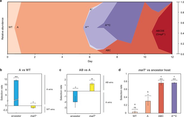
J evolution (a) and evidence of the interdependency between λ and E. coli fitness during their coevolution (b-d).
(a) Phylogenetic reconstruction and relative abundance of λ genotypes isolated through time from a previously coevolved community (Meyer et al., 2012). Each letter and star indicate a non-synonymous mutation in J (see Supplementary file 1c for labels’ corresponding mutations). A genotype’s relative abundance on a given day is denoted by the fraction of the total height of the y-axis that it occupies (e.g. on day 9, frequency of ABC is 0.2 and A**C is 0.8; see Supplementary file 1d). The lineage WT-A-ABC-ABCDE eventually evolves OmpF function and fixes in the population; resistance in E. coli through malT— rises to high frequencies between days 5 and 8 (Meyer et al., 2012). (b & c) Selection rates (per 24 hr) of phage genotypes on the two hosts. Each bar represents the mean of three experimental replicates. While mutation A is favored over wildtype (WT) λ in the presence of the ancestral host and not malT—, AB only outcompetes A in the presence of malT— and not the ancestral host. One tailed t-tests to test if the mean selection rate is significantly greater (or less) than zero: A vs WT with ancestor host- ; A vs WT with malT— - ; AB vs A with ancestor- ; AB vs A with malT— - . (d) Selection rate (per 4 hr) of malT– E. coli relative to its ancestor in the presence of λ from different stages of coevolution. Each competition was replicated three times. Lowercase letters denote significance via Tukey’s honest significance test, see Supplementary file 1g for pairwise p-values (ANOVA: F-ratio=111.22, d.f.=11, p<0.0001). One tailed t-tests were also used to test if the selection rate of malT— was greater than zero WT: ; A: ; ABC: ; A**C: . This shows that malT— is unlikely to evolve in the presence of WT λ but it becomes progressively more likely as λ gains mutations. Asterisks over all the competitions indicate significance level corresponding to the p-values. Error bars in all bar graphs represent one sample SD.
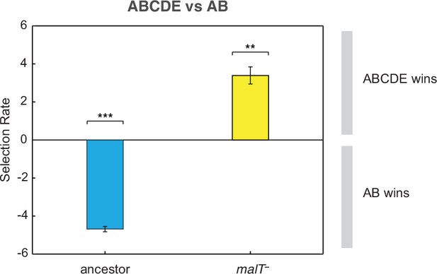
Competition assay of λ isolates from population D7.
Relative fitness of λ with two mutations (AB) to an OmpF+ λ with five mutations (ABCDE) on two host genotypes. This shows that AB outcompetes ABCDE in the presence of ancestral E. coli while ABCDE is favored over AB with malT— E. coli. Selection rate (per 4 hr) is the difference in Malthusian growth rates of the competitors over 1 day with a value of 0 indicating no difference in fitness. Each bar represents mean of three replicate trials and error bars indicate one sample SD. (One-tailed t-test to test if the selection rate is greater (or less) than zero— ABCDE vs AB with ancestor host: , ABCDE vs AB with malT—: . Asterisks over the bar graphs indicate significance level corresponding to the p-values).

Evolutionary replay experiments reveal that λ’s evolution to use OmpF depends on host coevolution.
(a) Wildtype (WT) λ with ancestral host, (b) WT λ with malT–, (c) λ one mutation removed from evolving OmpF function with malT—, and (d) identical setup as (c), but with λ two mutations removed (see Supplementary file 1f for identity of mutations). (e) The bar graph provides the frequency of OmpF+ evolution compared to the frequency observed by Meyer et al., 2012. Given λ’s established one in four rates of OmpF+ with ancestral host, the probability of observing no OmpF+ evolution in 12 replicate populations is ~0.03. Thus, no positives for OmpF evolution in (b) shows that λ’s evolution to OmpF function is significantly hindered, when coevolution is initiated with malT— host. However, malT— does not impede OmpF+ evolution, when the coevolution is initiated with already evolved λs (p-values for Fisher’s exact test: between (b) and (c) p=0.0261; between (b) and (d) p=0.0122). Notably, some λ populations went extinct which is common for these experiments and was previously shown to be caused by the evolution of resistance mutations in E. coli’s ManXYZ protein complex (Meyer et al., 2012).

A schematic overview of the coevolution experiments performed in this study and by Meyer et al., 2012.
Coevolution is initiated by coculturing λ and E. coli in glucose media for 24 hr at 37°C. At the end of each day, 1% of the total population is transferred to fresh media to continue the coevolution and the spent media is discarded. A fraction of the community is also sampled for long-term storage at −80°C, to determine population densities and to check the status of λ’s OmpF use.
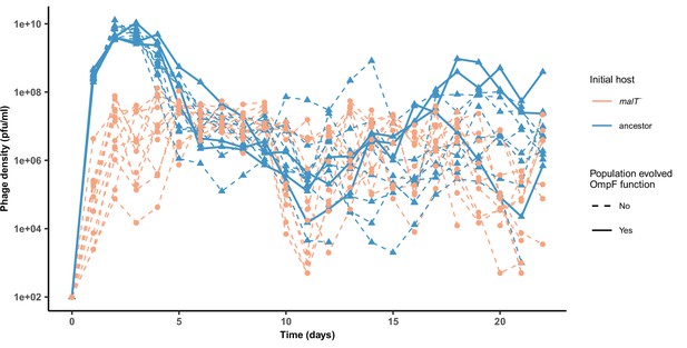
Phage densities during the coevolutionary replay experiment performed in Figure 4.
Timeseries of phage density of 12 replicates measured at the end of each day for cultures initiated with WT λ and ancestor host or malT— host (corresponding to Figure 4a, b). The three λ populations that evolved OmpF function in the ancestor host treatment are marked by solid lines. For the simulations, we used a populations size of 6.3 × 10⁹ which is lower than the peak population density observed (~1010), but above the average population density (~6.3 × 10⁸).
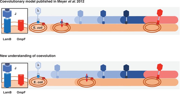
Previous and new version of λ-E. coli coevolutionary model.
In the original model, E. coli evolves resistance by repressing λ’s receptor and then λ evolves mutations that allow it to use a new receptor. The updated model describes a more involved dynamic where λ evolves mutations that improve its ability to infect E. coli; with increased pressure to avoid infection, E. coli responds by evolving resistance, and then λ evolves the remaining mutations that leads to the ability to infect using the new receptor.
Additional files
-
Supplementary file 1
All the supplementary tables.
- https://cdn.elifesciences.org/articles/76162/elife-76162-supp1-v1.docx
-
Transparent reporting form
- https://cdn.elifesciences.org/articles/76162/elife-76162-transrepform1-v1.docx


