A scalable and modular automated pipeline for stitching of large electron microscopy datasets
Figures
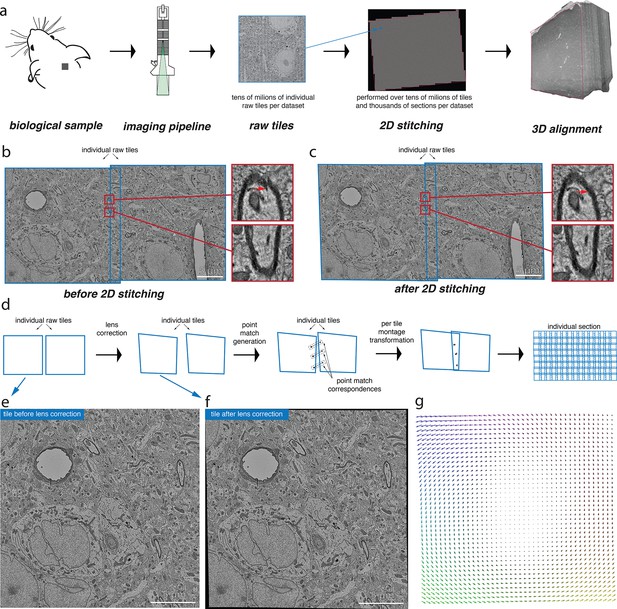
Volume assembly pipeline.
(a) Different stages of the electron microscopy (EM) dataset collection pipeline. The biological sample is prepared and cut into thin slices that are imaged using the desired image acquisition system (electron microscopy for datasets discussed in this work). The raw tile images from each section are then stitched together in 2D followed by a 3D alignment of them. (b) A pair of raw tile images before 2D stitching. The tiles have a certain overlap between them and are not aligned (the zoomed-in regions show the misalignment) and hence require a per-tile transformation to stitch them together. (c) The pair of tile images from (b) after stitching is performed. The zoomed-in regions illustrate the alignment of these images after stitching. (d) Conceptual diagram illustrating the series of steps that are involved in the 2D stitching of the serial sections. The steps include computation of lens distortion correction transformation followed by generation of point correspondences between the overlapping tile images and, finally, computation of per-tile montage transformations using the point correspondences. (e) A raw tile image without any lens distortion correction. (f) Tile image from (e) after lens distortion correction transformation is applied. (g) A quiver plot showing the magnitude and direction of distortion caused by the lens from the acquisition system.
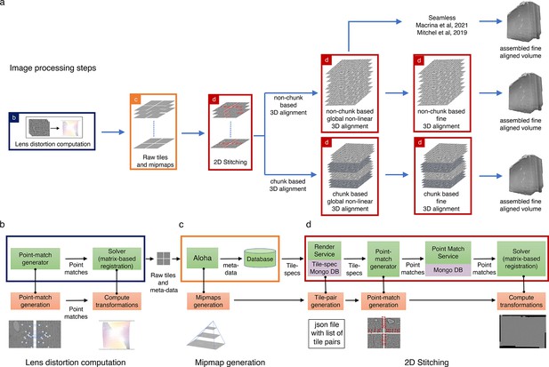
Assembly Stitching and Alignment Pipeline (ASAP) – volume assembly workflow.
(a) The different steps of image processing in ASAP for electron microscopy (EM) serial sections. The infrastructure permits multiple possible strategies for 3D alignment, including a chunk-based approach in case it is not possible to 3D align the complete dataset at once, as well as using other workflows outside ASAP (Macrina et al., 2021; https://www.microns-explorer.org/cortical-mm3) for fine 3D alignment with the global 3D aligned volume obtained using ASAP. (b–d) Representation of different modules in the software infrastructure. The green boxes represent software components, the orange boxes represent processes, and the purple processes represent databases. The color of the outline of the box matches its representation in the image processing steps shown in (a). (b) Schematic showing the lens distortion computation. (c) Schematic describing the process of data transfer and storage along with MIPmaps generation using the data transfer service Aloha. (d) Schematic illustrating the montaging process of serial sections. The same software infrastructure of (d) is then also used for 3D alignment as shown by the red boxes in (a).
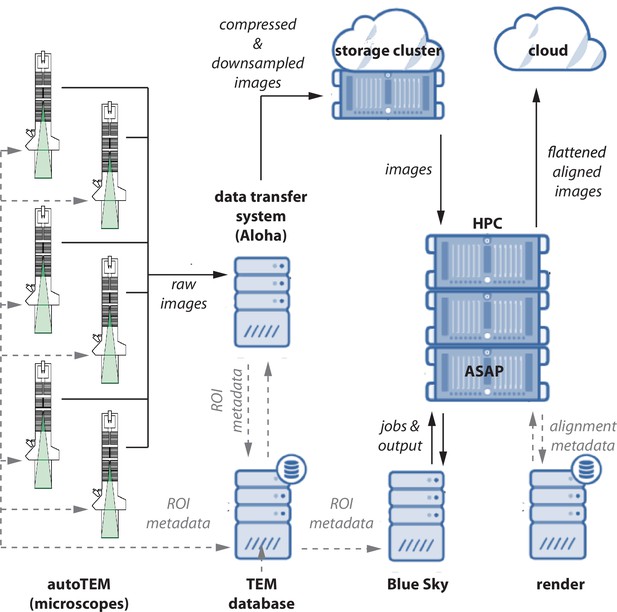
Data flow diagram.
A schematic diagram showing the flow of image data, metadata, and processed data between microscopes. Raw images and metadata are transferred from microscopes to our data transfer system (Aloha) and transmission electron microscopy (TEM) database, respectively. Aloha generates MIPmaps and compresses images and transfers them to the storage cluster for further processing by ASAP. Metadata is transferred to BlueSky through TEM database, which triggers the stitching and alignment process. The metadata from the stitching process is saved in the Render services database. The final assembled volume is transferred to the cloud for further fine alignment and segmentation. The hardware configurations are presented in Appendix 5.
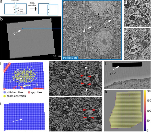
2D stitching and automated assessment of montage quality.
(a) Schematic diagram of the montage transformation using point correspondences. (b) Montage 2D stitched section from mouse dataset 1 (publicly available at https://www.microns-explorer.org; MICrONS Consortium et al., 2021). (c) Single-acquisition tile from the section in (b). (d, e) Detail of synapses (arrow heads) from the tile shown in (c). (f) Quality control (QC) plot of a stitched electron microscopy (EM) serial section with nonoptimal parameters. Each blue square represents a tile image of how they appear aligned in the montage. The red squares represent tile images that have gaps in stitching with neighboring tile images and are usually located in regions with resin or film. (g) A zoom-in region of the 2D montage in (f) showing the seam (white arrows) between tiles causing misalignment (red arrowheads) between membranes. (h) A zoomed-in region of the section showing a tile having a gap with its neighbors. (i) QC plot of a stitched EM serial section after parameter optimization. (j) A zoom-in region of the 2D montage in (i) showing no seams in the same region as in (g). The red arrowheads show the same locations as in (g). (k) A schematic plot representing the number of point correspondences between every pair of tile images for a section of the human dataset. Each edge of the squares in the plot represents the existence of point correspondences between tile images centered at the end points of the edge. The color of the edge represents the number of point correspondences computed between those tile image pairs.
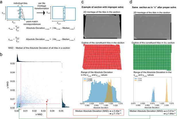
Median absolute deviation (MAD) statistics for montage distortion detection.
(a) Schematic description of computation of MAD statistics for a montage. (b) A scatter plot of and MAD values for each montage. A good stitched section without distorted tile images falls in the third quadrant (where point d is shown). (c) An example of a distorted montage of a section solved using unoptimized set of parameters. Row 1 shows the downsampled version of the montaged section, row 2 shows the quality control (QC) plot of the section showing the distortions, and row 3 shows the and absolute deviation distribution for the unoptimized montage. (d) Section shown in (c) solved with optimized parameters with row 1 showing the downsampled montage, row 2 showing the QC plot of the section, and row 3 showing the and absolute deviation distribution for the section.
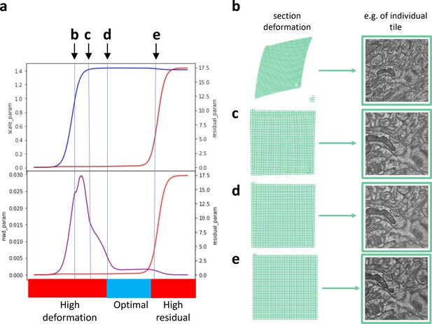
Parameter optimization.
(a) Plots showing the residuals (red curve) with variations in the scale parameter (blue curve) and median absolute deviation (MAD) parameter (purple curve). The optimal solve occurs between (d) and (e) in the figure. A high MAD value indicates deformation of the tiles and is consistent with the scale changes to the tile outline images. An optimal set of solver parameters that produce a low MAD and residuals are selected for montaging. (b) Representation of a serial section with each square representing a tile image. The section shows significant deformations when solved with unoptimal parameters (location b in [a]). (c) The same serial section from (b) solved with parameters in the region pointed by c in (a). (d) The same serial section from (b) solved with parameters in the region pointed by d in (a). (e) The same serial section from (b) solved with optimal set of parameters from the region pointed by e in (a). The tile images shown in the last column show the quality of solve from each of these parameter sets.
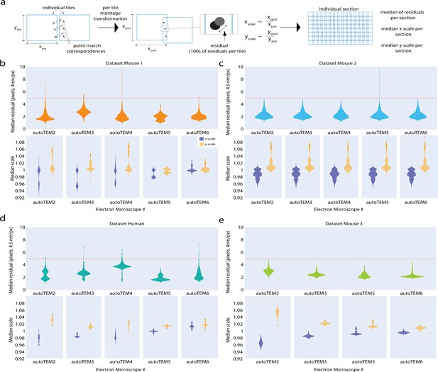
Performance of 2D stitching pipeline.
(a) Schematic diagram explaining the computation of residuals between a pair of tile images post stitching. Residuals is a metric that is used to assess the quality of stitching in our pipeline. (b–e, top): panels (b–e) show the median of tile residuals per section grouped by their acquisition transmission electron microscopy (TEM). The horizontal line in these figures marks the threshold value that is set to assess the quality of stitching. Table 2 shows the median residual values in nm for all our datasets. (b–e , bottom): panels (b–e) show the median and scale distribution of the tile images for all the datasets grouped by their acquisition system. The and scales of the tile images post 2D stitching indicate the level of deformation that a tile image undergoes post stitching – an indicator of the degree of quality of the 2D montaged section. (b) Mouse dataset 1. (c) Mouse dataset 2. (d) Human dataset. (e) Mouse dataset 3.
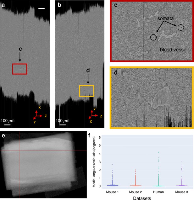
Global nonlinear 3D aligned volume of the mouse dataset 1.
(a) View of the global nonlinear 3D aligned volume from the plane. The figure shows the view of the global nonlinear 3D alignment of the sections with the volume sliced at position marked by the red lines in (e). (b) View of the global nonlinear 3D aligned volume from the plane. Figure shows the view of the volume sliced at position marked by the red lines in (e). (c) Zoomed-in area from (a) showing the quality of global nonlinear 3D alignment in the plane. (d) Zoomed-in area from (b) showing the quality of global nonlinear 3D alignment in the plane. (e) Maximum pixel intensity projection of the global nonlinear 3D aligned sections in the z-axis showing the overall alignment of sections within the volume. The red lines represent the slicing location in both and plane for the cross-sectional slices shown in (a) and (b). (f) A plot showing the distribution of median angular residuals from serial sections grouped by the dataset.
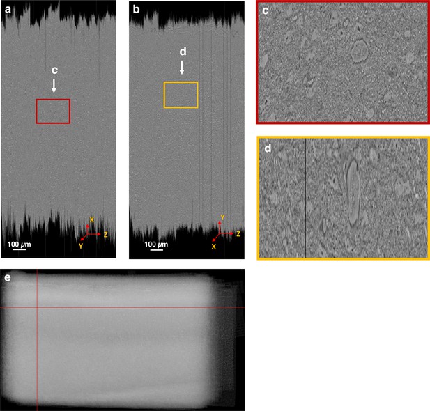
Global nonlinear 3D aligned volume of the mouse dataset 2.
(a) View of the global nonlinear 3D aligned volume from the xz plane. The figure shows the view of the global nonlinear 3D alignment of the sections with the volume sliced at position marked by the red lines in (e). (b) View of the global nonlinear 3D aligned volume from the yz plane. Figure shows the view of the volume sliced at position marked by the red lines in (e). (c) Zoomed-in area from (a) showing the quality of global nonlinear 3D alignment in the xz plane. (d) Zoomed-in area from (b) showing the quality of global nonlinear 3D alignment in the yz plane. (e) Maximum pixel intensity projection of the global nonlinear 3D aligned sections in the z-axis showing the overall alignment of sections within the volume. The red lines represent the slicing location in both xz and yz plane for the cross-sectional figures in (a) and (b).
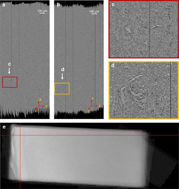
Global nonlinear 3D aligned volume of the human dataset.
(a) View of the global nonlinear 3D aligned volume from the xz plane. The figure shows the view of the global nonlinear 3D alignment of the sections with the volume sliced at position marked by the red lines in (e). (b) View of the global nonlinear 3D aligned volume from the yz plane. Figure shows the view of the volume sliced at position marked by the red lines in (e). (c) Zoomed-in area from (a) showing the quality of global nonlinear 3D alignment in the xz plane. (d) Zoomed-in area from (b) showing the quality of global nonlinear 3D alignment in the yz plane. (e) Maximum pixel intensity projection of the global nonlinear 3D aligned sections in the z-axis showing the overall alignment of sections within the volume. The red lines represent the slicing location in both xz and yz plane for the cross-sectional figures in (a) and (b).
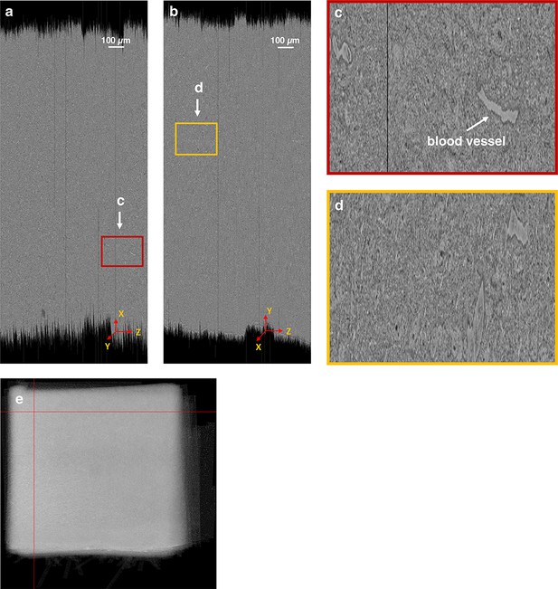
Global nonlinear 3D aligned volume of the mouse dataset 3.
(a) View of the global nonlinear 3D aligned volume from the xz plane. The figure shows the view of the global nonlinear 3D alignment of the sections with the volume sliced at position marked by the red lines in (e). (b) View of the global nonlinear 3D aligned volume from the yz plane. Figure shows the view of the volume sliced at position marked by the red lines in (e). (c) Zoomed-in area from (a) showing the quality of global nonlinear 3D alignment in the xz plane. (d) Zoomed-in area from (b) showing the quality of global nonlinear 3D alignment in the yz plane. (e) Maximum pixel intensity projection of the global nonlinear 3D aligned sections in the z-axis showing the overall alignment of sections within the volume. The red lines represent the slicing location in both xz and yz plane for the cross-sectional figures in (a) and (b).
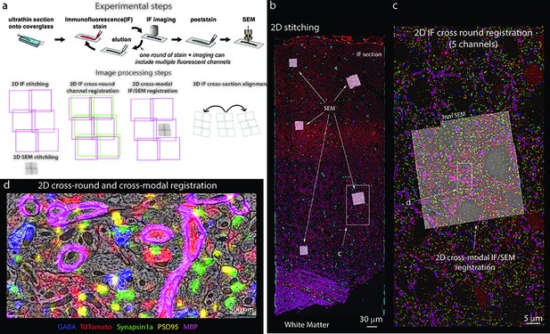
Stitching of multichannel conjugate array tomography data.
(a, top) Experimental steps in conjugate array tomography: Serial sections are collected onto glass coverslips and exposed to multiple rounds of immunofluorescent (IF) staining, imaging, and elution, followed by post-staining and imaging under a field emission scanning electron microscopy (FESEM). (a, bottom) Schematic illustrating the substeps of image processing large-scale conjugate array tomography data. 2D stitching must be performed on each round of IF imaging and EM imaging. Multiple rounds of IF imaging of the same physical section must be registered together to form a highly multiplexed IF image of that section. The higher resolution by typically smaller spatial scale FESEM data must then be registered to the lower resolution but larger spatial scale IF data for each individual 2D section and FESEM montage. Finally, alignments of the data across sections must be calculated from the IF, or alternatively EM datasets. In all cases, the transformations of each of these substeps must be composed to form a final coherent multimodal, multiresolution representation of the dataset. (b–d) Screenshots of a processed dataset, rendered dynamically in Neuroglancer through the Render web services. (b) An overview image of a single section of conjugate array tomography data that shows the result of stitching and registering multiple rounds of IF an EM data. Channels shown are GABA (blue), TdTomato (Red), Synapsin1a (green), PSD95 (yellow), and MBP (purple). Small white box highlights the region shown in (c). (c) A zoom-in of one area of the section where FESEM data was acquired, small white box shows the detailed region shown in (d). (d) A high-resolution view of an area of FESEM data with IF data overlaid on top. One can observe the tight correspondence between the locations of IF signals and corresponding ultrastructural correlates, such a myelinated axons on MBP, and postsynaptic densities and PSD95.
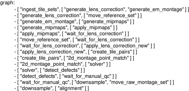
Intelligence Advanced Research Projects Activity (IARPA) MICrONS phase 2 montage workflow with support for lens correction and manual intervention.
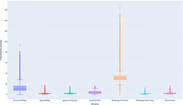
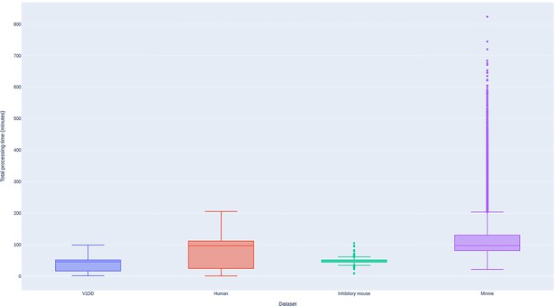
Performance of BlueSky workflow manager.
Time spent by the sections from all the datasets in each job queue in the montaging workflow. The processing times include the duration between the time the job started running in a node and the time the node releases the job as successfully completed. Processing times shown are based on running the job in a single computing node in every job queue.
Tables
Details of datasets processed using Assembly Stitching and Alignment Pipeline (ASAP) – volume assembly pipeline.
| Dataset | No. of sections | Pixel resolution (nm/pixel) | Image size | Tile overlap | Total size (PiB) | Total size (nonoverlap) (PiB) | ROI size (in microns) |
|---|---|---|---|---|---|---|---|
| Mouse dataset 1 | 19,945 | 3.95–4 | (20MP camera), (50MP camera) | 13%, 9% | 1.6 | 1.2 | |
| Mouse dataset 2 | 17,593 | 4.67–5 (4.78 mean) | 9–10%, 9.4% mean | 0.984 | 0.807 | ||
| Mouse dataset 3 | 17,310 | 3.8–4.15 (3.91 mean) | 9–10%, 9.1% mean | 0.665 | 0.549 | ||
| Human | 9673 | 4.65–4.95 (4.78 mean) | 9–10%, 9.5% mean | 1.18 | 0.968 |
-
ROI, region of interest.
Performance of 2D stitching pipeline.
Table shows the values of metrics computed to assess the quality of the stitched montages from all our datasets. The median residual value and the median scale in the x-axis and y-axis measures the accuracy of the alignment and the deformation factor of the individual tile images.
| Dataset | Median residuals (pixels) | Median residuals (nm) | Median scale (x) | Median scale (y) |
|---|---|---|---|---|
| Human dataset | 2.59 | 12.38 | 0.98 | 1.02 |
| Mouse dataset 1 | 2.10 | 8.36 | 0.99 | 1.00 |
| Mouse dataset 2 | 2.21 | 10.56 | 0.98 | 1.00 |
| Mouse dataset 3 | 2.37 | 9.27 | 0.99 | 1.01 |
Processing time comparison between acquisition system and Assembly Stitching and Alignment Pipeline (ASAP).
The acquisition times shown are based on serial sections imaged using five different serial section transmission electron microscopies (ssTEMs) running in parallel. The stitching time for all the datasets includes the time it took to stitch all the serial sections including semi-automated quality control (QC) and reprocessing sections that failed QC on the first run and the global 3D alignment. The stitching was done in a noncontinuous fashion that included correctly uploading/reuploading corrupted, duplicate sections, etc. Each section was stitched using a single node from the compute cluster. The different processing times of the different datasets reflect the optimization of the pipeline over time, while still keeping a throughput in pace with imaging acquisition.
| Dataset | No. of sections | Acquisition time (months) | ASAP processing time (includes manual processing times) |
|---|---|---|---|
| Mouse dataset 1 | 26,500 | 6 | 4 months |
| Mouse dataset 2 | 17,584 | 3 | 6 weeks |
| Human dataset | 9,661 | 2 | 4 weeks |
| Mouse dataset 3 | 17,309 | 3 | 10 days |


