COVID-19 pandemic dynamics in South Africa and epidemiological characteristics of three variants of concern (Beta, Delta, and Omicron)
- Department of Epidemiology, Mailman School of Public Health, Columbia University, United States
- Department of Environmental Health Sciences, Mailman School of Public Health, Columbia University, United States
Figures
Figure 1
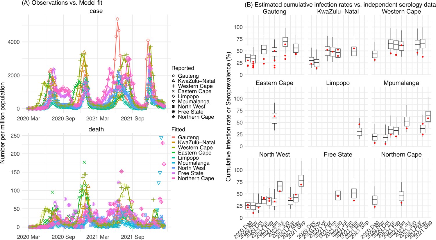
Pandemic dynamics in South Africa, model-fit and validation using serology data.
(A) Pandemic dynamics in each of the nine provinces (see legend); dots depict reported weekly numbers of cases and deaths; lines show model mean estimates (in the same color). (B) For validation, model estimated infection rates are compared to seroprevalence measures over time from multiple sero-surveys summarized in The South African COVID-19 Modelling Consortium, 2021. Boxplots depict the estimated distribution for each province (middle bar = mean; edges = 50% CrIs) and whiskers (95% CrIs), summarized over n=100 model-inference runs (500 model replica each, totaling 50,000 model realizations). Red dots show corresponding measurements. Note that reported mortality was high in February 2022 in some provinces (see additional discussion in Appendix 1).
Figure 2
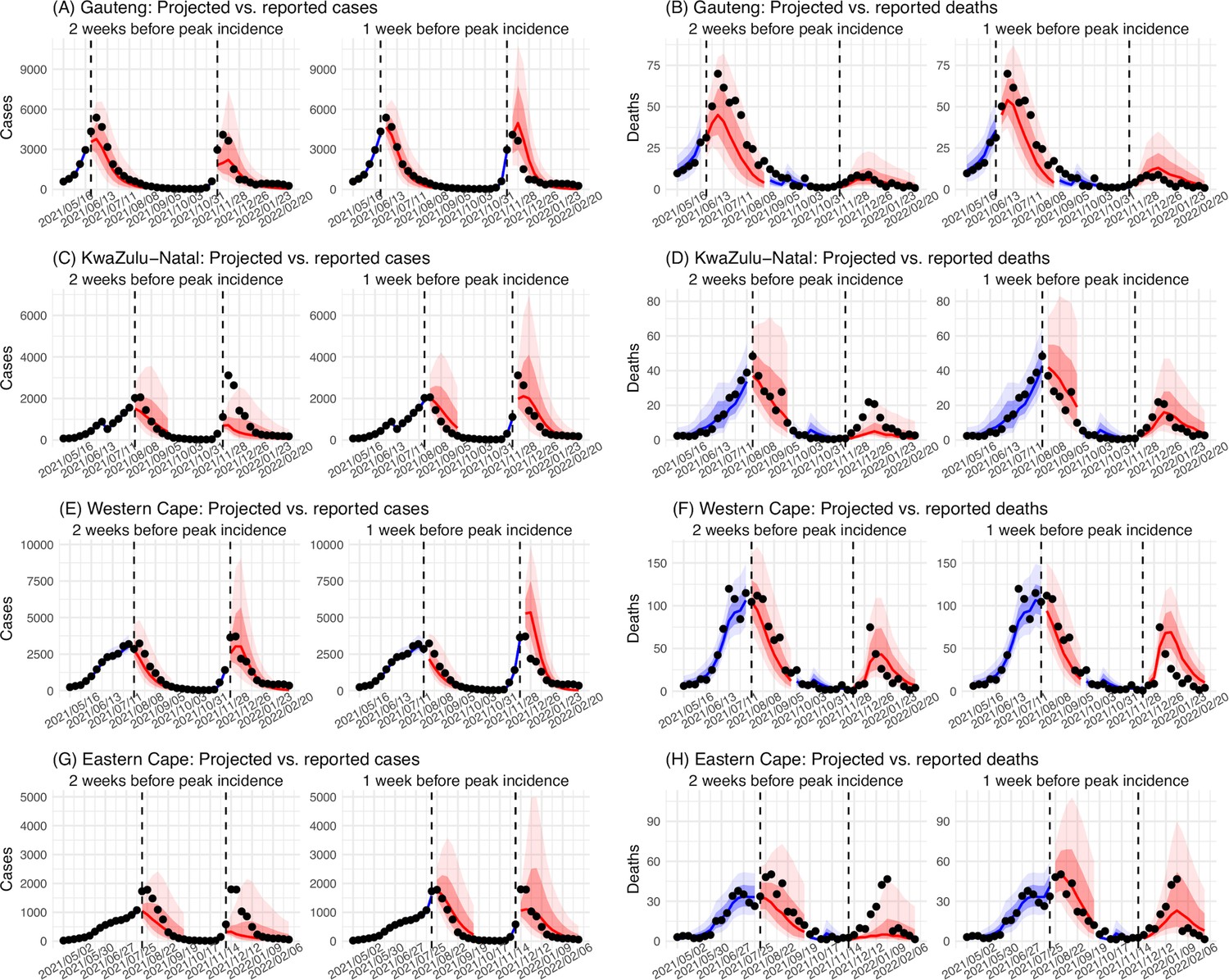
Model validation using retrospective prediction.
Model-inference was trained on cases and deaths data since March 15, 2020 until 2 weeks (1st plot in each panel) or 1 week (2nd plot) before the Delta or Omicron (BA.1) wave (see timing on the x-axis); the model was then integrated forward using the estimates made at the time to predict cases (left panel) and deaths (right panel) for the remaining weeks of each wave. Blue lines and surrounding shades show model fitted cases and deaths for weeks before the prediction (line = median, dark blue area = 50% CrIs, and light blue = 80% CrIs, summarized over n=100 model-inference runs totaling 50,000 model realizations). Red lines show model projected median weekly cases and deaths; surrounding shades show 50% (dark red) and 80% (light red) CIs of the prediction (n = 50,000 model realizations). For comparison, reported cases and deaths for each week are shown by the black dots; however, those to the right of the vertical dash lines (showing the start of each prediction) were not used in the model. For clarity, here we show 80% CIs (instead of 95% CIs, which tend to be wider for longer-term projections) and predictions for the four most populous provinces (Gauteng in A and B; KwaZulu-Natal in C and D; Western Cape in E and F; and Eastern Cape in G and H). Predictions for the other five provinces are shown in Appendix 1—figure 3.
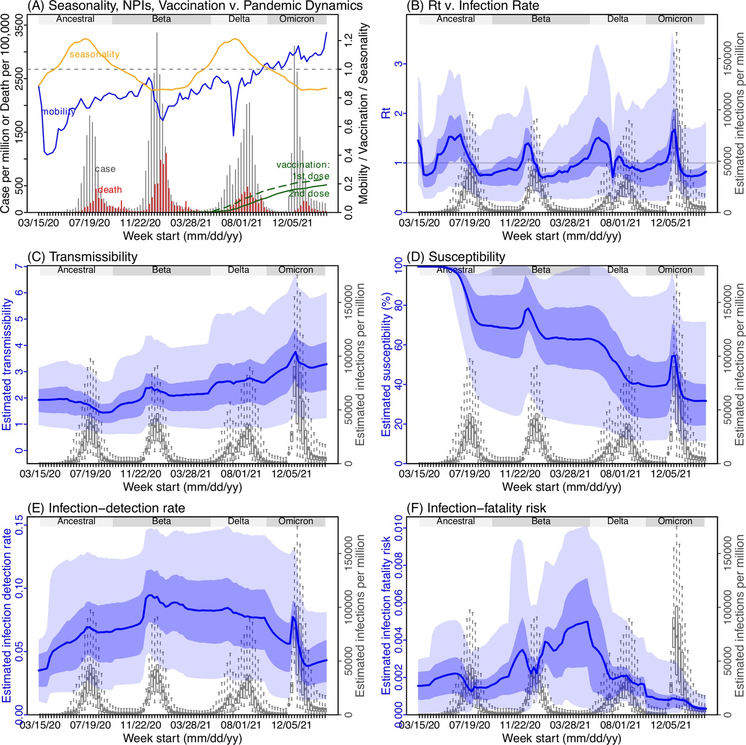
Figure 3
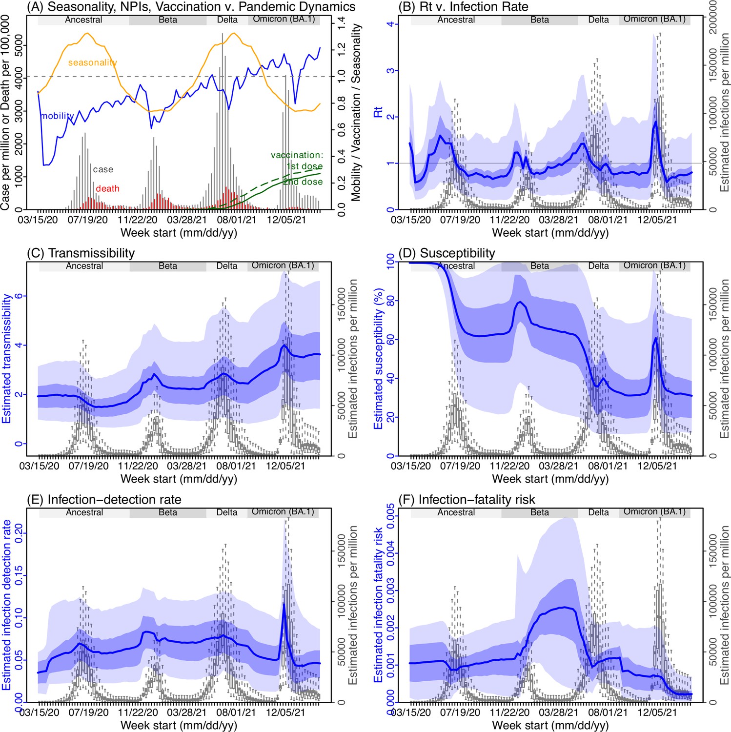
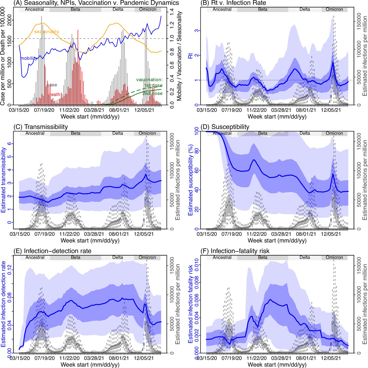
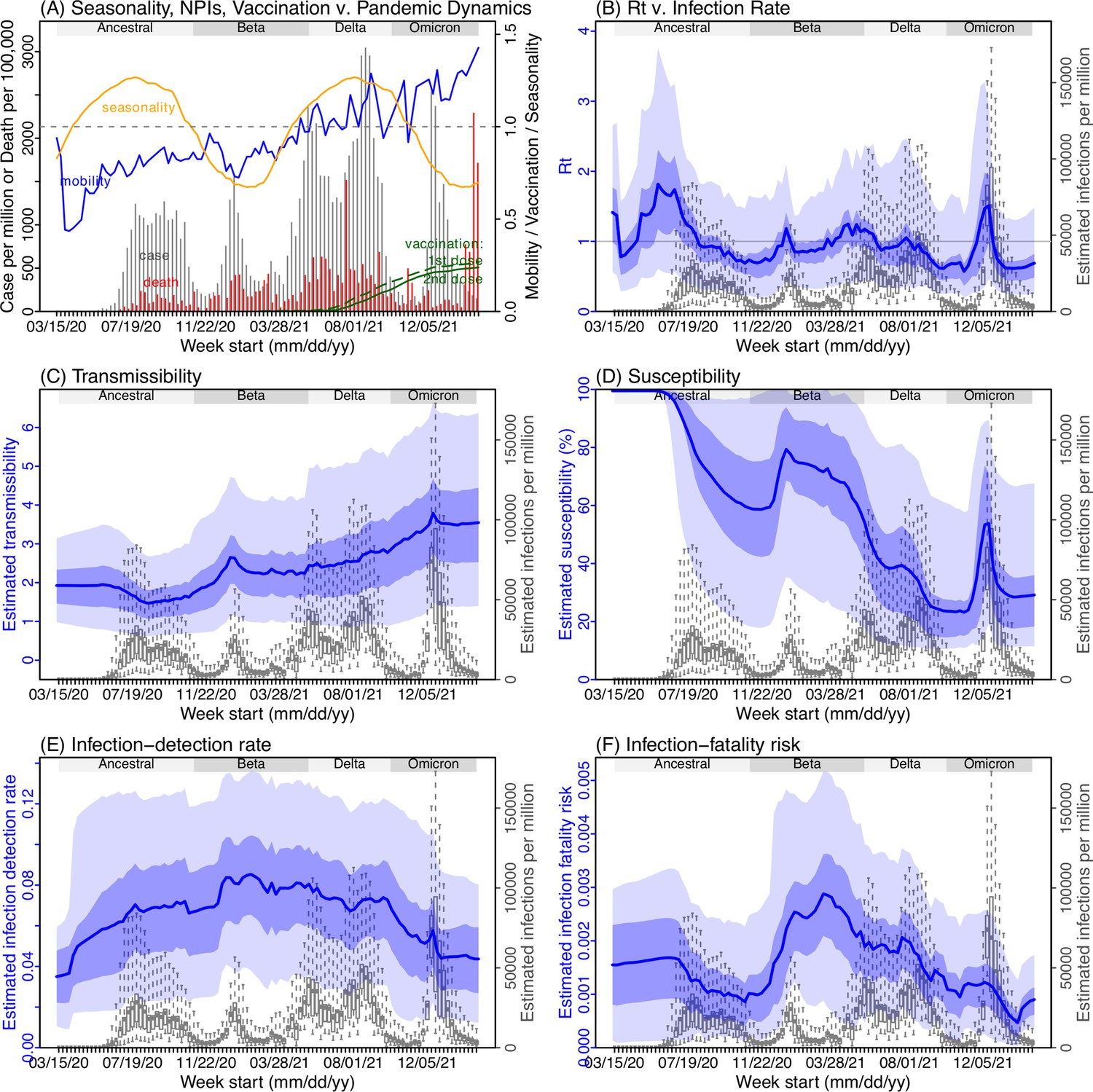
Example model-inference estimates for Gauteng.
(A) Observed relative mobility, vaccination rate, and estimated disease seasonal trend, compared to case and death rates over time. Key model-inference estimates are shown for the time-varying effective reproduction number Rt (B), transmissibility RTX (C), population susceptibility (D, shown relative to the population size in percentage), infection-detection rate (E), and infection-fatality risk (F). Grey shaded areas indicate the approximate circulation period for each variant. In (B) – (F), blue lines and surrounding areas show the estimated mean, 50% (dark) and 95% (light) CrIs; boxes and whiskers show the estimated mean, 50% and 95% CrIs for estimated infection rates. All summary statistics are computed based on n=100 model-inference runs totaling 50,000 model realizations. Note that the transmissibility estimates (RTX in C) have removed the effects of changing population susceptibility, NPIs, and disease seasonality; thus, the trends are more stable than the reproduction number (Rt in B) and reflect changes in variant-specific properties. Also note that infection-fatality risk estimates were based on reported COVID-19 deaths and may not reflect true values due to likely under-reporting of COVID-19 deaths.
Figure 4
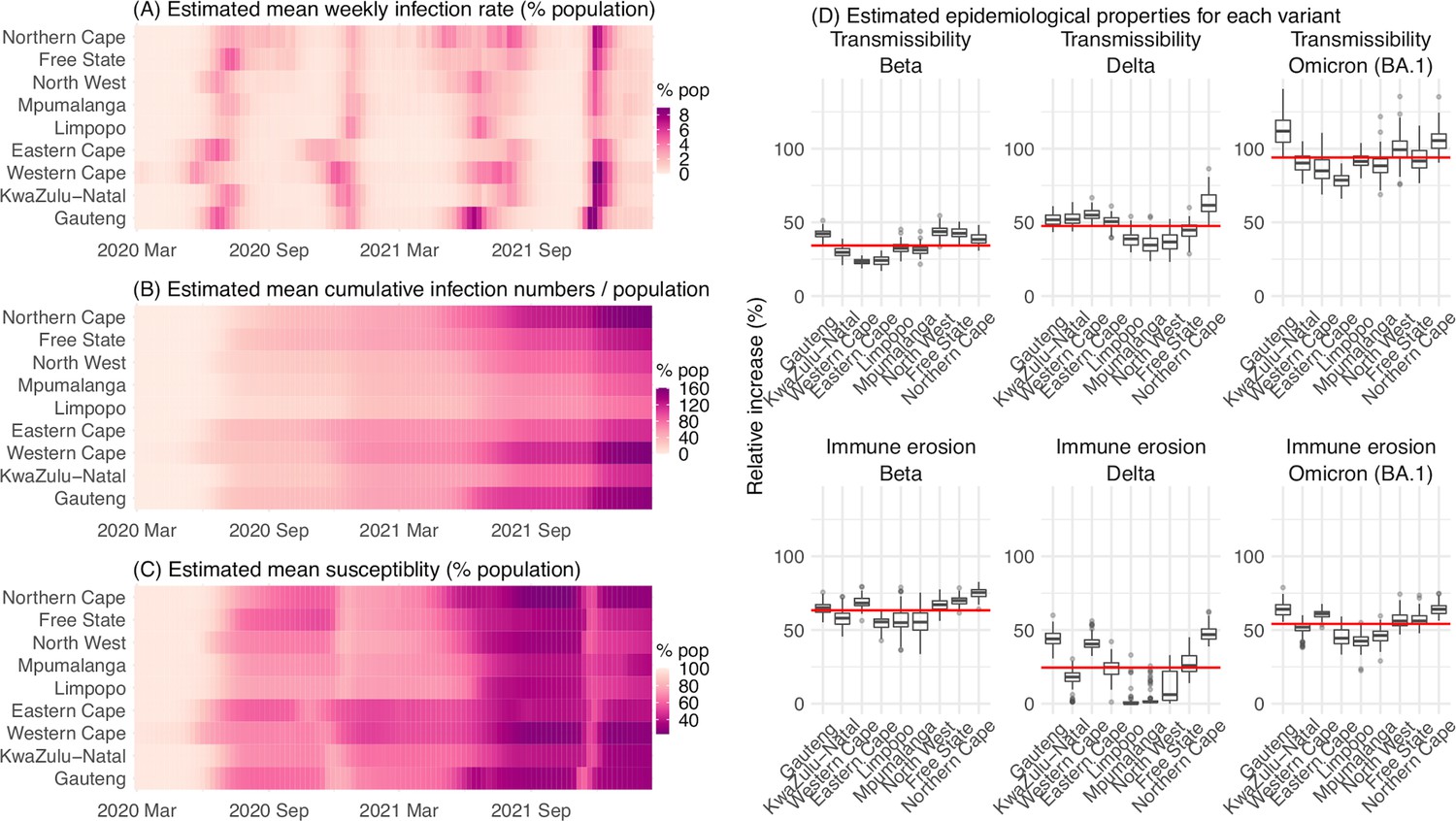
Model-inferred epidemiological properties for different variants across SA provinces.
Heatmaps show (A) Estimated mean infection rates by week (x-axis) and province (y-axis), (B) Estimated mean cumulative infection numbers relative to the population size in each province, and (C) Estimated population susceptibility (to the circulating variant) by week and province. (D) Boxplots in the top row show the estimated distribution of increases in transmissibility for Beta, Delta, and Omicron (BA.1), relative to the Ancestral SARS-CoV-2, for each province (middle bar = median; edges = 50% CIs; and whiskers = 95% CIs; summarized over n=100 model-inference runs); boxplots in the bottom row show, for each variant, the estimated distribution of immune erosion to all adaptive immunity gained from infection and vaccination prior to that variant. Red lines show the mean across all provinces.
Appendix 1—figure 1
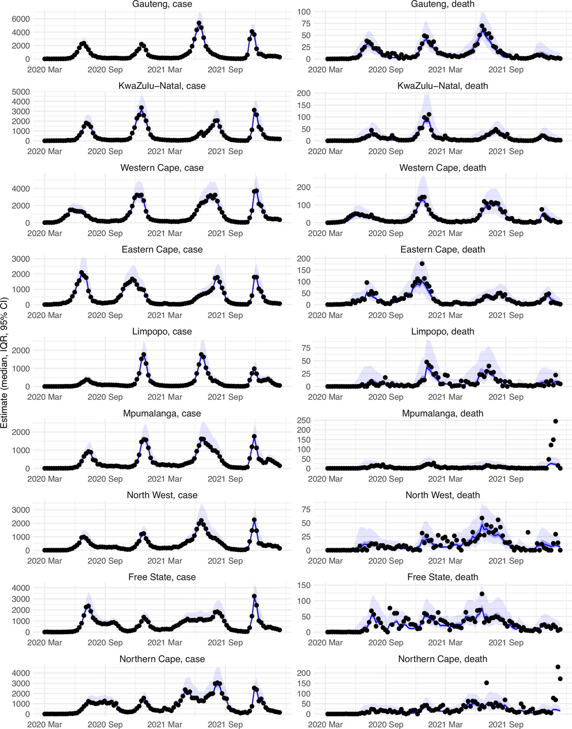
Model-fit to case and death data in each province.
Dots show reported SARS-CoV-2 cases and deaths by week. Blue lines and surrounding area show model estimated median, 50% (darker blue) and 95% (lighter blue) credible intervals. Note that reported mortality was high in February 2022 in some provinces with no clear explanation.
Appendix 1—figure 2
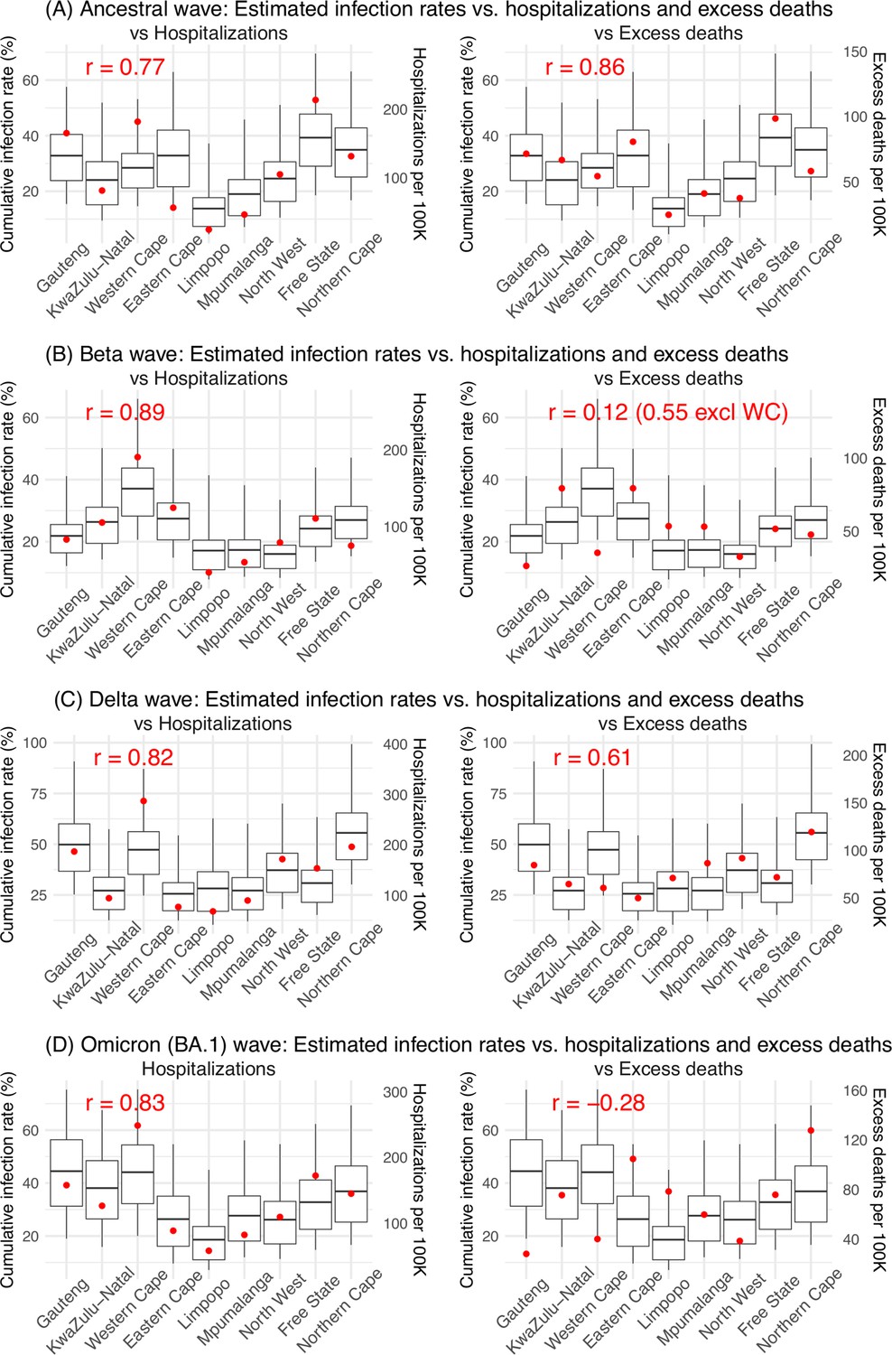
Model validation using hospitalization and excess mortality data.
Model estimated infection rates are compared to COVID-related hospitalizations (left panel) and excess mortality (right panel) during the Ancestral (A), Beta (B), Delta (C), and Omicron (D) waves. Boxplots show the estimated distribution for each province (middle bar = mean; edges = 50% CrIs and whiskers = 95% CrIs). Red dots show COVID-related hospitalizations (left panel, right y-axis) and excess mortality (right panel, right y-axis); these are independent measurements not used for model fitting. Correlation (r) is computed between model estimates (i.e., median cumulative infection rates for the nine provinces) and the independent measurements (i.e., hospitalizations in the nine provinces in left panel, and age-adjusted excess mortality in the right panel), for each wave. Note that hospitalization data begin from 6/6/20 and excess mortality data begin from 5/3/20 and thus are incomplete for the ancestral wave.
Appendix 1—figure 3
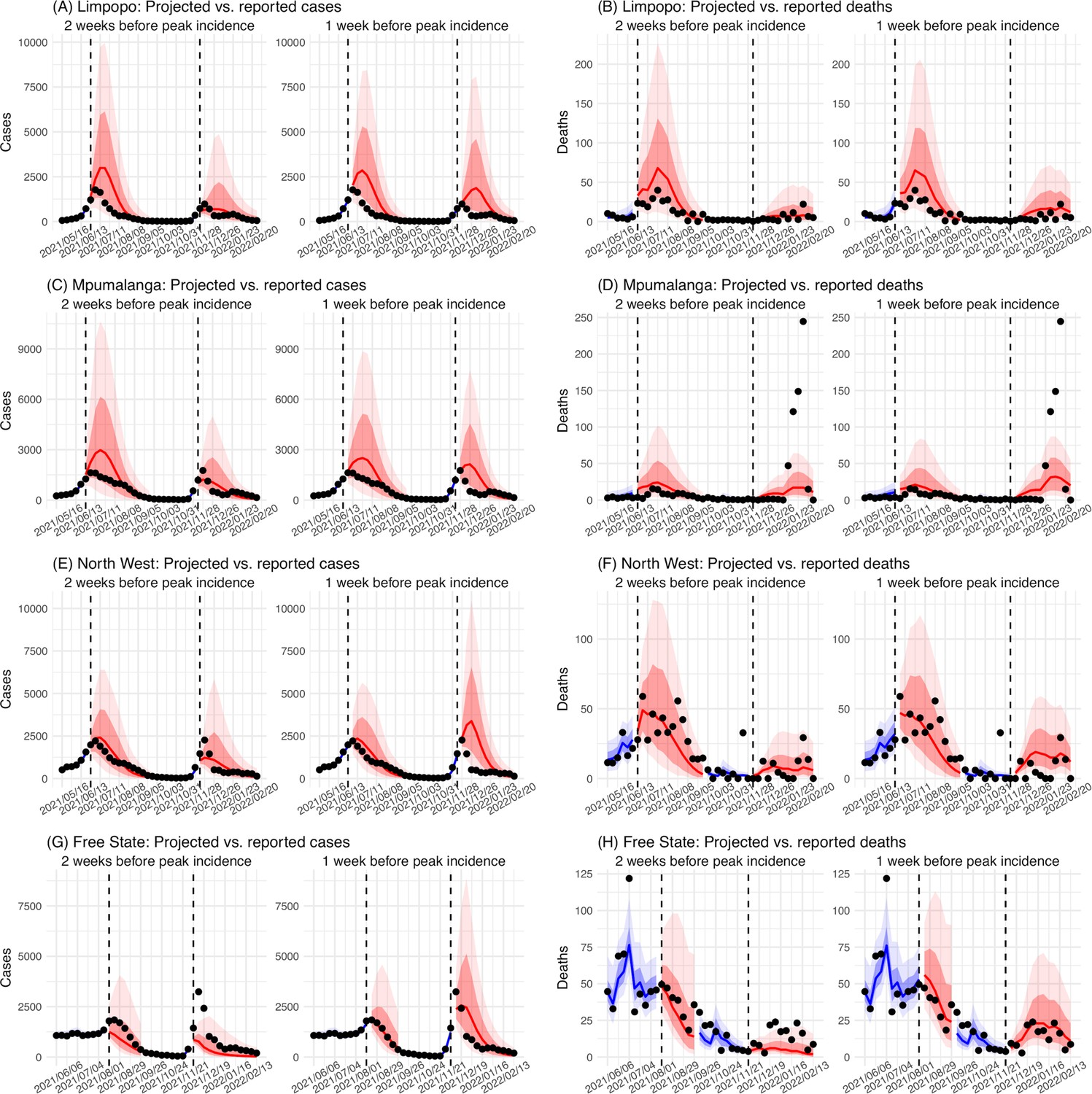
Model validation using retrospective prediction, for the remaining 5 provinces.
Model-inference was trained on cases and deaths data since March 15, 2020 until 2 weeks (1st plot in each panel) or 1 week (2nd plot) before the Delta or Omicron wave (see timing on the x-axis); the model was then integrated forward using the estimates made at the time to predict cases (left panel) and deaths (right panel) for the remaining weeks of each wave. Blue lines and surrounding shades show model fitted cases and deaths for weeks before the prediction (line = median, dark blue area = 50% CrIs, and light blue = 80% CrIs). Red lines show model projected median weekly cases and deaths; surrounding shades show 50% (dark red) and 80% (light red) CIs of the prediction. For comparison, reported cases and deaths for each week are shown by the black dots; however, those to the right of the vertical dash lines (showing the start of each prediction) were not used in the model. For clarity, here we show 80% CIs (instead of 95% CIs, which tend to be wider for longer-term projections) and predictions for the five least populous provinces (Limpopo in A and B; Mpumalanga in C and D; North West in E and F; Free State in G and H; and Northern Cape in I and J). Predictions for the other 4 provinces are shown in Figure 2.
Appendix 1—figure 4
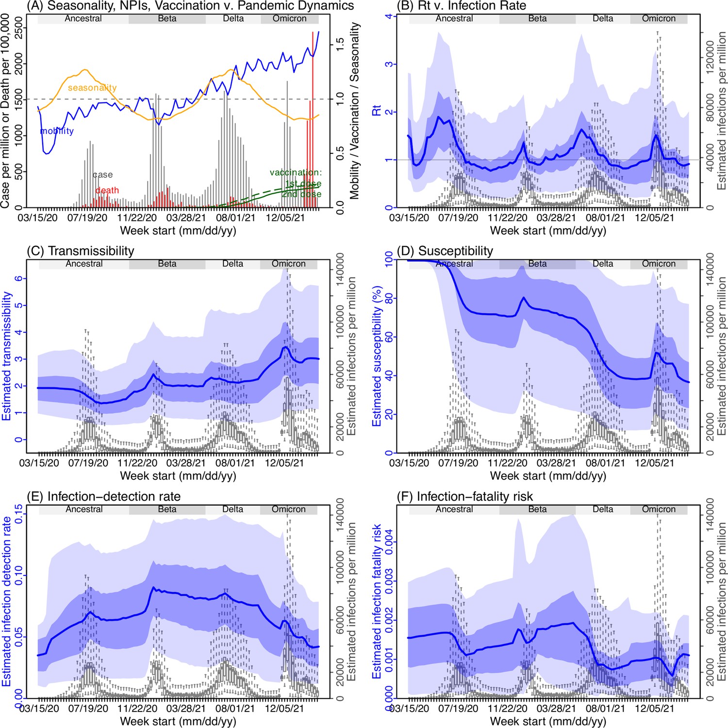
Model inference estimates for KwaZulu-Natal.
(A) Observed relative mobility, vaccination rate, and estimated disease seasonal trend, compared to case and death rates over time. Key model-inference estimates are shown for the time-varying effective reproduction number Rt (B), transmissibility RTX (C), population susceptibility (D, shown relative to the population size in percentage), infection-detection rate (E), and infection-fatality risk (F). Grey shaded areas indicate the approximate circulation period for each variant. In (B) – (F), blue lines and surrounding areas show the estimated mean, 50% (dark) and 95% (light) CrIs; boxes and whiskers show the estimated mean, 50% and 95% CrIs for estimated infection rates. Note that the transmissibility estimates (RTX in C) have removed the effects of changing population susceptibility, NPIs, and disease seasonality; thus, the trends are more stable than the reproduction number (Rt in B) and reflect changes in variant-specific properties. Also note that infection-fatality risk estimates were based on reported COVID-19 deaths and may not reflect true values due to likely under-reporting of COVID-19 deaths.
Appendix 1—figure 5

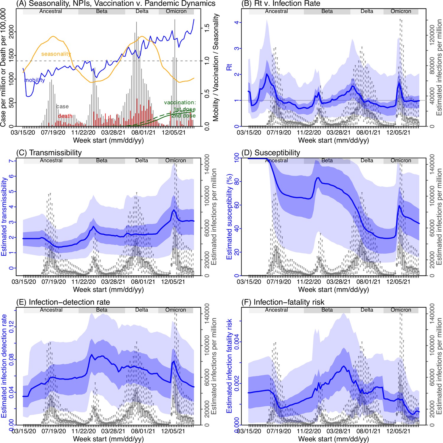
Model inference estimates for Western Cape.
(A) Observed relative mobility, vaccination rate, and estimated disease seasonal trend, compared to case and death rates over time. Key model-inference estimates are shown for the time-varying effective reproduction number Rt (B), transmissibility RTX (C), population susceptibility (D, shown relative to the population size in percentage), infection-detection rate (E), and infection-fatality risk (F). Grey shaded areas indicate the approximate circulation period for each variant. In (B) – (F), blue lines and surrounding areas show the estimated mean, 50% (dark) and 95% (light) CrIs; boxes and whiskers show the estimated mean, 50% and 95% CrIs for estimated infection rates. Note that the transmissibility estimates (RTX in C) have removed the effects of changing population susceptibility, NPIs, and disease seasonality; thus, the trends are more stable than the reproduction number (Rt in B) and reflect changes in variant-specific properties. Also note that infection-fatality risk estimates were based on reported COVID-19 deaths and may not reflect true values due to likely under-reporting of COVID-19 deaths.
Appendix 1—figure 6
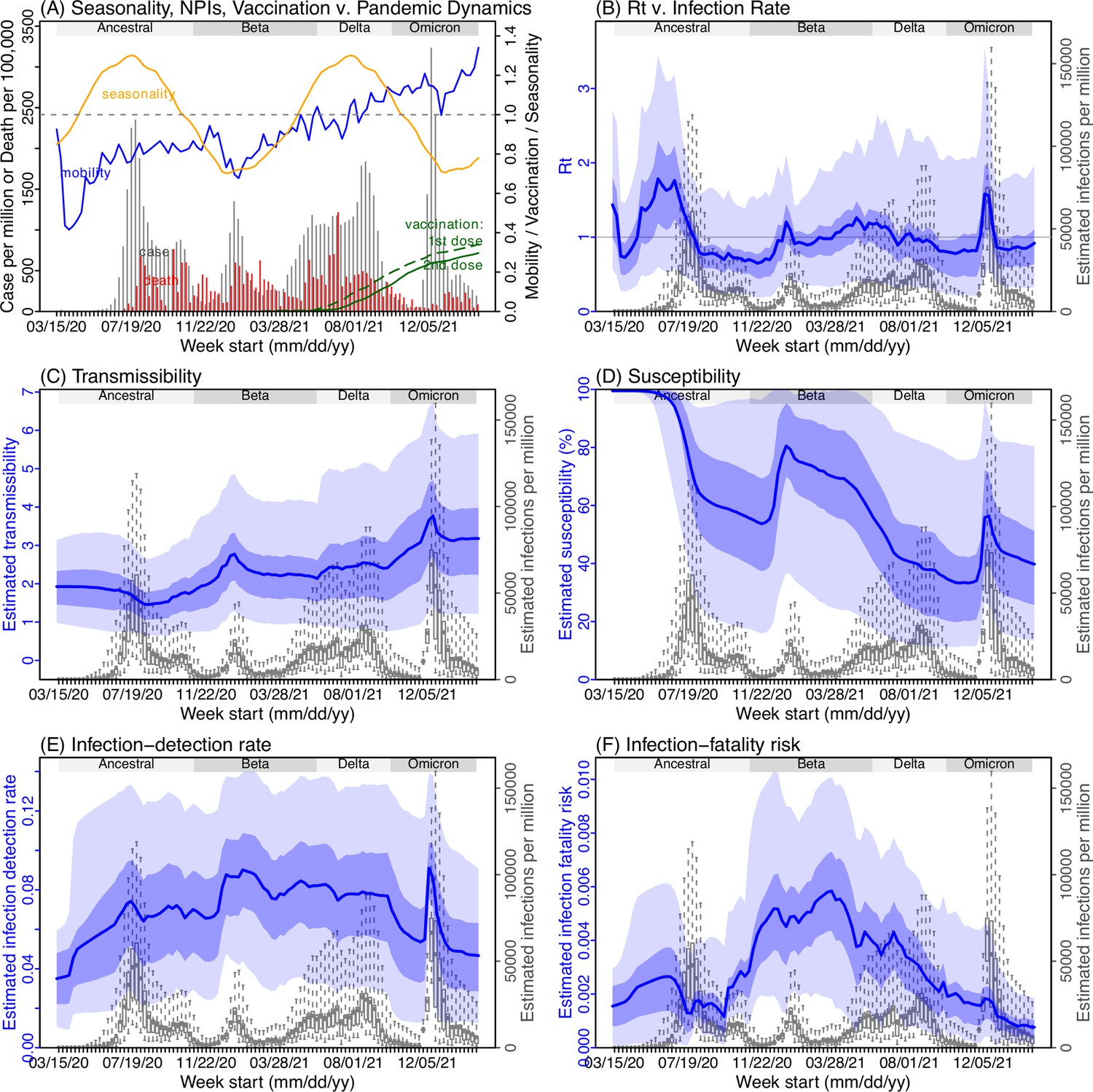
Model inference estimates for Eastern Cape.
(A) Observed relative mobility, vaccination rate, and estimated disease seasonal trend, compared to case and death rates over time. Key model-inference estimates are shown for the time-varying effective reproduction number Rt (B), transmissibility RTX (C), population susceptibility (D, shown relative to the population size in percentage), infection-detection rate (E), and infection-fatality risk (F). Grey shaded areas indicate the approximate circulation period for each variant. In (B) – (F), blue lines and surrounding areas show the estimated mean, 50% (dark) and 95% (light) CrIs; boxes and whiskers show the estimated mean, 50% and 95% CrIs for estimated infection rates. Note that the transmissibility estimates (RTX in C) have removed the effects of changing population susceptibility, NPIs, and disease seasonality; thus, the trends are more stable than the reproduction number (Rt in B) and reflect changes in variant-specific properties. Also note that infection-fatality risk estimates were based on reported COVID-19 deaths and may not reflect true values due to likely under-reporting of COVID-19 deaths.
Appendix 1—figure 7

Model inference estimates for Limpopo.
(A) Observed relative mobility, vaccination rate, and estimated disease seasonal trend, compared to case and death rates over time. Key model-inference estimates are shown for the time-varying effective reproduction number Rt (B), transmissibility RTX (C), population susceptibility (D, shown relative to the population size in percentage), infection-detection rate (E), and infection-fatality risk (F). Grey shaded areas indicate the approximate circulation period for each variant. In (B) – (F), blue lines and surrounding areas show the estimated mean, 50% (dark) and 95% (light) CrIs; boxes and whiskers show the estimated mean, 50% and 95% CrIs for estimated infection rates. Note that the transmissibility estimates (RTX in C) have removed the effects of changing population susceptibility, NPIs, and disease seasonality; thus, the trends are more stable than the reproduction number (Rt in B) and reflect changes in variant-specific properties. Also note that infection-fatality risk estimates were based on reported COVID-19 deaths and may not reflect true values due to likely under-reporting of COVID-19 deaths.
Appendix 1—figure 8
Model inference estimates for Mpumalanga.
(A) Observed relative mobility, vaccination rate, and estimated disease seasonal trend, compared to case and death rates over time. Key model-inference estimates are shown for the time-varying effective reproduction number Rt (B), transmissibility RTX (C), population susceptibility (D, shown relative to the population size in percentage), infection-detection rate (E), and infection-fatality risk (F). Grey shaded areas indicate the approximate circulation period for each variant. In (B) – (F), blue lines and surrounding areas show the estimated mean, 50% (dark) and 95% (light) CrIs; boxes and whiskers show the estimated mean, 50% and 95% CrIs for estimated infection rates. Note that the transmissibility estimates (RTX in C) have removed the effects of changing population susceptibility, NPIs, and disease seasonality; thus, the trends are more stable than the reproduction number (Rt in B) and reflect changes in variant-specific properties. Also note that infection-fatality risk estimates were based on reported COVID-19 deaths and may not reflect true values due to likely under-reporting of COVID-19 deaths.
Appendix 1—figure 9
Model inference estimates for North West.
(A) Observed relative mobility, vaccination rate, and estimated disease seasonal trend, compared to case and death rates over time. Key model-inference estimates are shown for the time-varying effective reproduction number Rt (B), transmissibility RTX (C), population susceptibility (D, shown relative to the population size in percentage), infection-detection rate (E), and infection-fatality risk (F). Grey shaded areas indicate the approximate circulation period for each variant. In (B) – (F), blue lines and surrounding areas show the estimated mean, 50% (dark) and 95% (light) CrIs; boxes and whiskers show the estimated mean, 50% and 95% CrIs for estimated infection rates. Note that the transmissibility estimates (RTX in C) have removed the effects of changing population susceptibility, NPIs, and disease seasonality; thus, the trends are more stable than the reproduction number (Rt in B) and reflect changes in variant-specific properties. Also note that infection-fatality risk estimates were based on reported COVID-19 deaths and may not reflect true values due to likely under-reporting of COVID-19 deaths.
Appendix 1—figure 10
Model inference estimates for Free State.
(A) Observed relative mobility, vaccination rate, and estimated disease seasonal trend, compared to case and death rates over time. Key model-inference estimates are shown for the time-varying effective reproduction number Rt (B), transmissibility RTX (C), population susceptibility (D, shown relative to the population size in percentage), infection-detection rate (E), and infection-fatality risk (F). Grey shaded areas indicate the approximate circulation period for each variant. In (B) – (F), blue lines and surrounding areas show the estimated mean, 50% (dark) and 95% (light) CrIs; boxes and whiskers show the estimated mean, 50% and 95% CrIs for estimated infection rates. Note that the transmissibility estimates (RTX in C) have removed the effects of changing population susceptibility, NPIs, and disease seasonality; thus, the trends are more stable than the reproduction number (Rt in B) and reflect changes in variant-specific properties. Also note that infection-fatality risk estimates were based on reported COVID-19 deaths and may not reflect true values due to likely under-reporting of COVID-19 deaths.
Appendix 1—figure 11
Model inference estimates for Northern Cape.
(A) Observed relative mobility, vaccination rate, and estimated disease seasonal trend, compared to case and death rates over time. Key model-inference estimates are shown for the time-varying effective reproduction number Rt (B), transmissibility RTX (C), population susceptibility (D, shown relative to the population size in percentage), infection-detection rate (E), and infection-fatality risk (F). Grey shaded areas indicate the approximate circulation period for each variant. In (B) – (F), blue lines and surrounding areas show the estimated mean, 50% (dark) and 95% (light) CrIs; boxes and whiskers show the estimated mean, 50% and 95% CrIs for estimated infection rates. Note that the transmissibility estimates (RTX in C) have removed the effects of changing population susceptibility, NPIs, and disease seasonality; thus, the trends are more stable than the reproduction number (Rt in B) and reflect changes in variant-specific properties. Also note that infection-fatality risk estimates were based on reported COVID-19 deaths and may not reflect true values due to likely under-reporting of COVID-19 deaths.
Appendix 1—figure 12

Comparison of posterior estimates for Gauteng during the Omicron (BA.1) wave, under four different settings for infection-detection rate.
Four space reprobing (SR) settings for the infection-detection rate were tested and results are shown in the 4 four columns: (1) Use of the same baseline range as before (i.e., 1%–8%) for all weeks during the Omicron (BA.1) wave; (2) Use of a wider and higher range (i.e., 1%–12%) for all weeks; (3) Use of a range of 1%–15% for the 1st week of Omicron detection, 5%–20% for the 2nd week of Omicron detection, and 1%–8% for the rest; and (4) Use of a range of 5%–25% for the 2nd week of detection and 1%–8% for all other weeks. Estimated infection-detection rates are shown in the 1st row, population susceptibility estimates are shown in the 2nd row, and transmissibility estimates are shown in the 3rd row. In each plot, blue lines and surrounding areas show the median, 50% and 95% CrIs of the posterior (left y-axis) for each week (x-axis). For comparison, reported cases for corresponding weeks are shown by the grey bars (right y-axis).
Appendix 1—figure 13
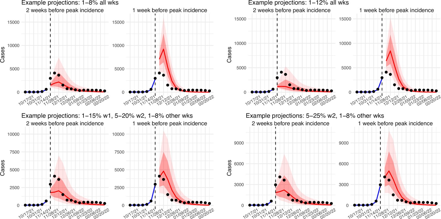
Comparison of retrospective prediction of the Omicron (BA.1) wave in Gauteng with the four different settings of infection-detection rate.
Four space reprobing (SR) settings for the infection-detection rate were tested, and the results are shown in the 4 panels: (1) Use of the same baseline range as before (i.e., 1%–8%) for all weeks during the Omicron (BA.1) wave; (2) Use of a wider and higher range (i.e., 1%–12%) for all weeks; (3) Use of a range of 1%–15% for the 1st week of Omicron detection, 5%–20% for the 2nd week of Omicron detection, and 1%–8% for the rest; and (4) Use of a range of 5%–25% for the 2nd week of detection and 1%–8% for all other weeks. Blue lines and show model fitted cases for weeks before the prediction. Red lines show model projected median weekly cases and deaths; surrounding shades show 50% (dark red) and 80% (light red) CIs of the prediction. For comparison, reported cases for each week are shown by the black dots; however, those to the right of the vertical dash lines (showing the start of each prediction) were not used in the model.
Appendix 1—figure 14
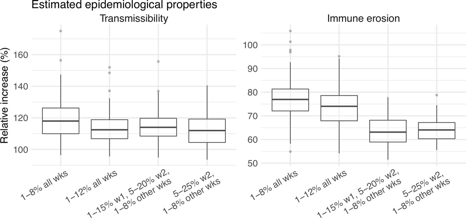
Comparison of the estimated increase in transmissibility and immune erosion for the Omicron (BA.1) variant in Gauteng, under four different settings of the infection-detection rate.
Four space reprobing (SR) settings for the infection-detection rate were tested: (1) Use of the same baseline range as before (i.e., 1%–8%) for all weeks during the Omicron (BA.1) wave; (2) Use of a wider and higher range (i.e., 1%–12%) for all weeks; (3) Use of a range of 1%–15% for the 1st week of Omicron detection, 5%–20% for the 2nd week of Omicron detection, and 1%–8% for the rest; and (4) Use of a range of 5%–25% for the 2nd week of detection and 1%–8% for all other weeks. Boxplots in left panel show the estimated distribution of increases in transmissibility, relative to the Ancestral SARS-CoV-2 (middle bar = median; edges = 50% CIs; and whiskers = 95% CIs); boxplots in the right panel show the estimated distribution of immune erosion to all adaptive immunity gained from infection and vaccination prior to the surge of Omicron (BA.1) wave.
Appendix 1—figure 15
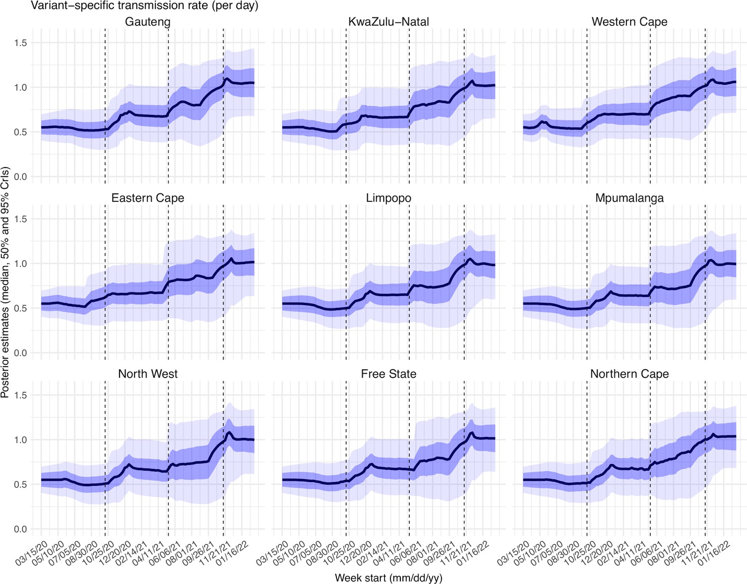
Posterior estimates for the transmission rate ( in Equation 1) by week.
Thick black lines show the median, dark blue areas show the 50% CrIs, and light blue areas show the 95% CrIs. For reference, the dashed vertical black lines indicate three dates (mm/dd/yy), that is 10/15/20, 5/15/21, and 11/15/21, roughly the start of the Beta, Delta, and Omicron waves, respectively.
Appendix 1—figure 16
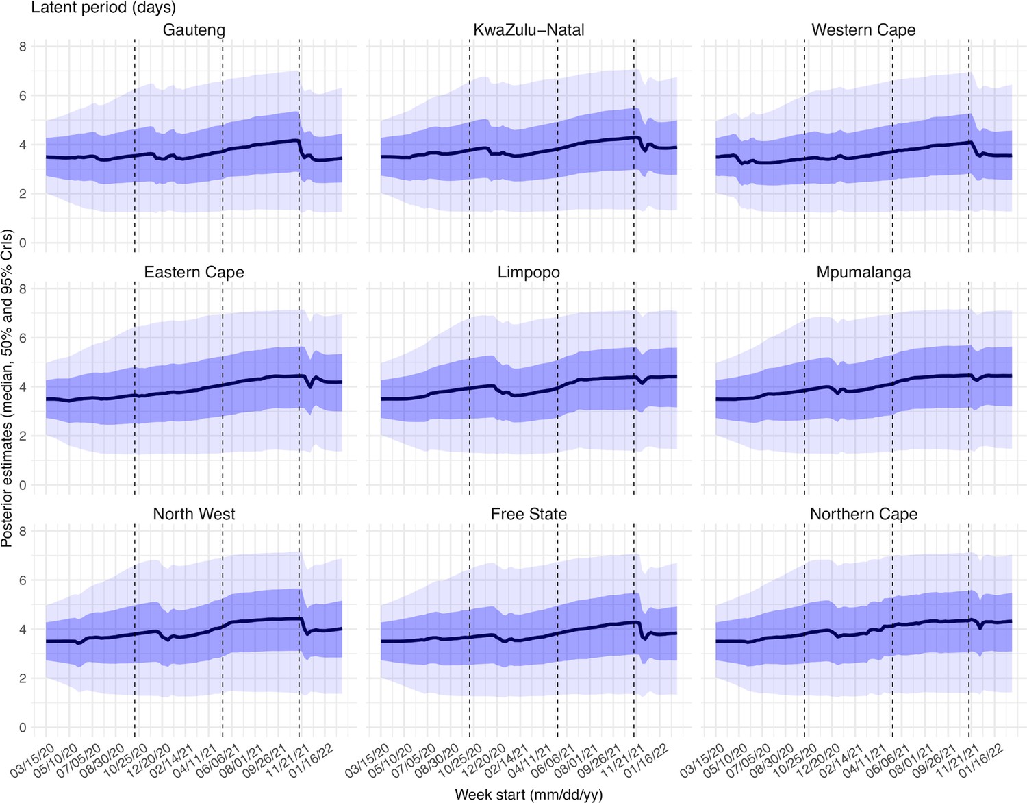
Posterior estimates for the latent period ( in Equation 1) by week.
Thick black lines show the median, dark blue areas show the 50% CrIs, and light blue areas show the 95% CrIs. For reference, the dashed vertical black lines indicate three dates (mm/dd/yy), i.e., 10/15/20, 5/15/21, and 11/15/21, roughly the start of the Beta, Delta, and Omicron waves, respectively.
Appendix 1—figure 17
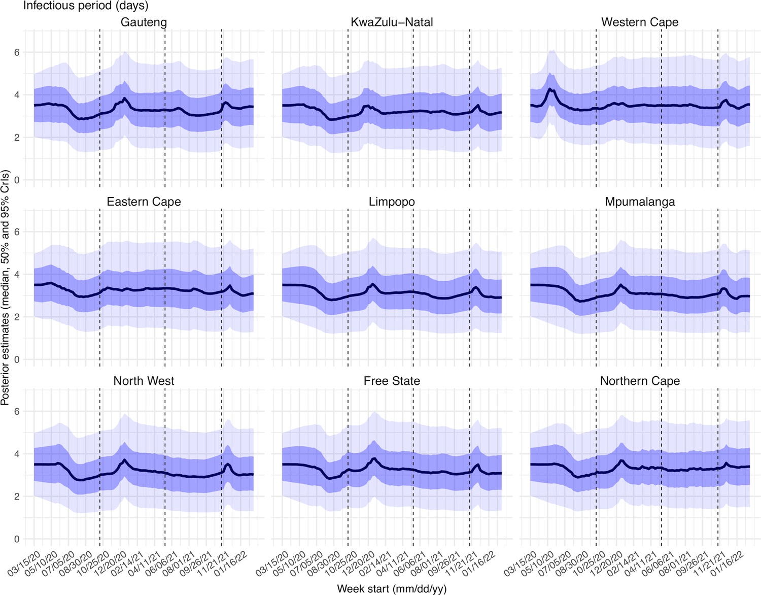
Posterior estimates for the infectious period ( in Equation 1) by week.
Thick black lines show the median, dark blue areas show the 50% CrIs, and light blue areas show the 95% CrIs. For reference, the dashed vertical black lines indicate three dates (mm/dd/yy), i.e., 10/15/20, 5/15/21, and 11/15/21, roughly the start of the Beta, Delta, and Omicron waves, respectively.
Appendix 1—figure 18

Posterior estimates for the immunity period ( in Equation 1) by week.
Thick black lines show the median, dark blue areas show the 50% CrIs, and light blue areas show the 95% CrIs. For reference, the dashed vertical black lines indicate three dates (mm/dd/yy), i.e., 10/15/20, 5/15/21, and 11/15/21, roughly the start of the Beta, Delta, and Omicron waves, respectively.
Appendix 1—figure 19
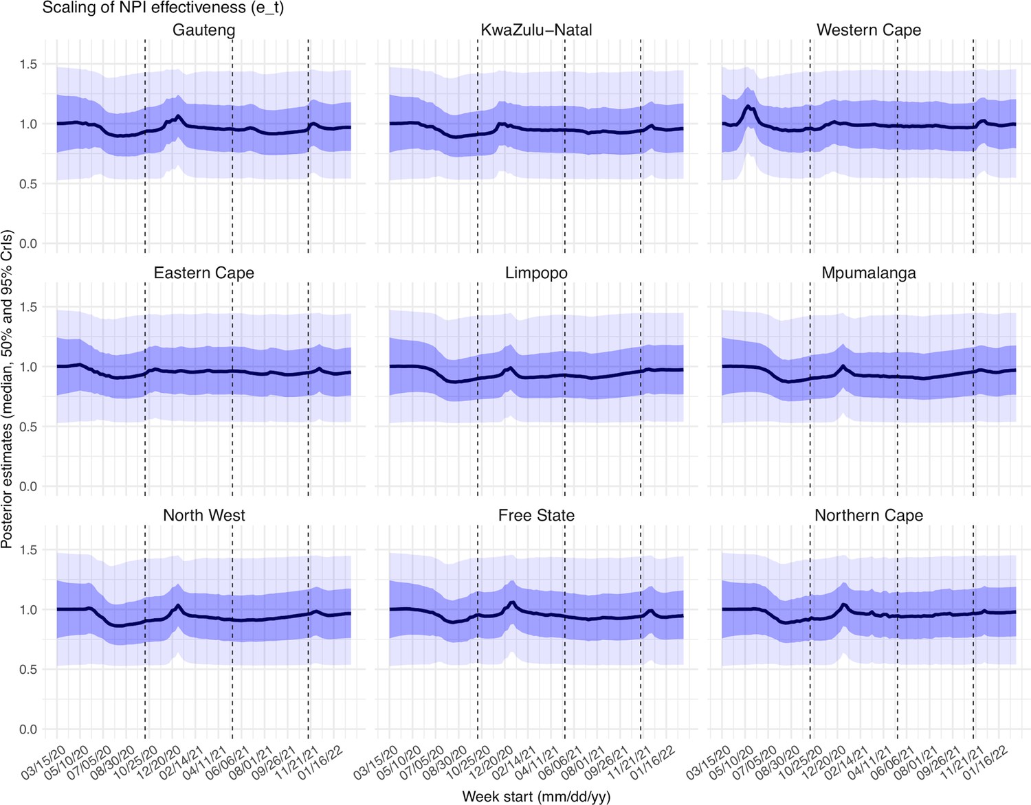
Posterior estimates for the scaling factor of NPI effectiveness ( in Equation 1) by week.
Thick black lines show the median, dark blue areas show the 50% CrIs, and light blue areas show the 95% CrIs. For reference, the dashed vertical black lines indicate three dates (mm/dd/yy), i.e., 10/15/20, 5/15/21, and 11/15/21, roughly the start of the Beta, Delta, and Omicron waves, respectively.
Appendix 1—figure 20
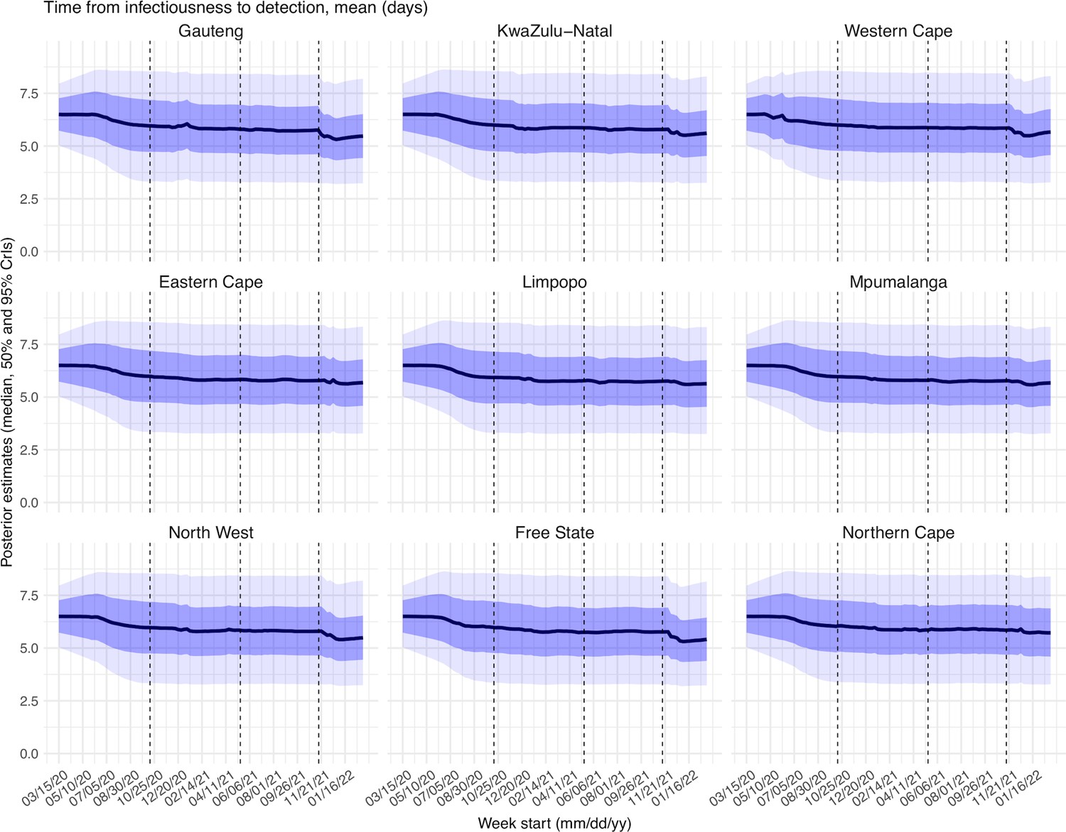
Posterior estimates for the mean of time from infectiousness to detection ( in the observation model) by week.
Thick black lines show the median, dark blue areas show the 50% CrIs, and light blue areas show the 95% CrIs. For reference, the dashed vertical black lines indicate three dates (mm/dd/yy), i.e., 10/15/20, 5/15/21, and 11/15/21, roughly the start of the Beta, Delta, and Omicron waves, respectively.
Appendix 1—figure 21
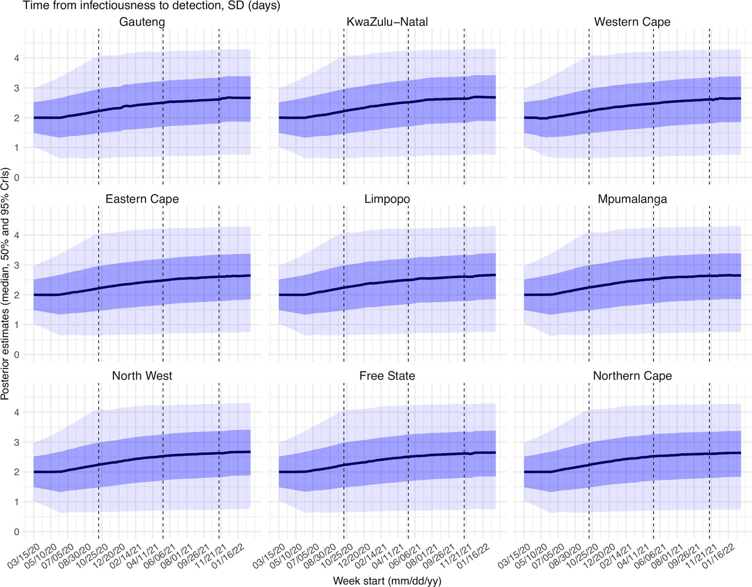
Posterior estimates for the standard deviation of time from infectiousness to detection ( in the observation model) by week.
Thick black lines show the median, dark blue areas show the 50% CrIs, and light blue areas show the 95% CrIs. For reference, the dashed vertical black lines indicate three dates (mm/dd/yy), i.e., 10/15/20, 5/15/21, and 11/15/21, roughly the start of the Beta, Delta, and Omicron waves, respectively.
Appendix 1—figure 22
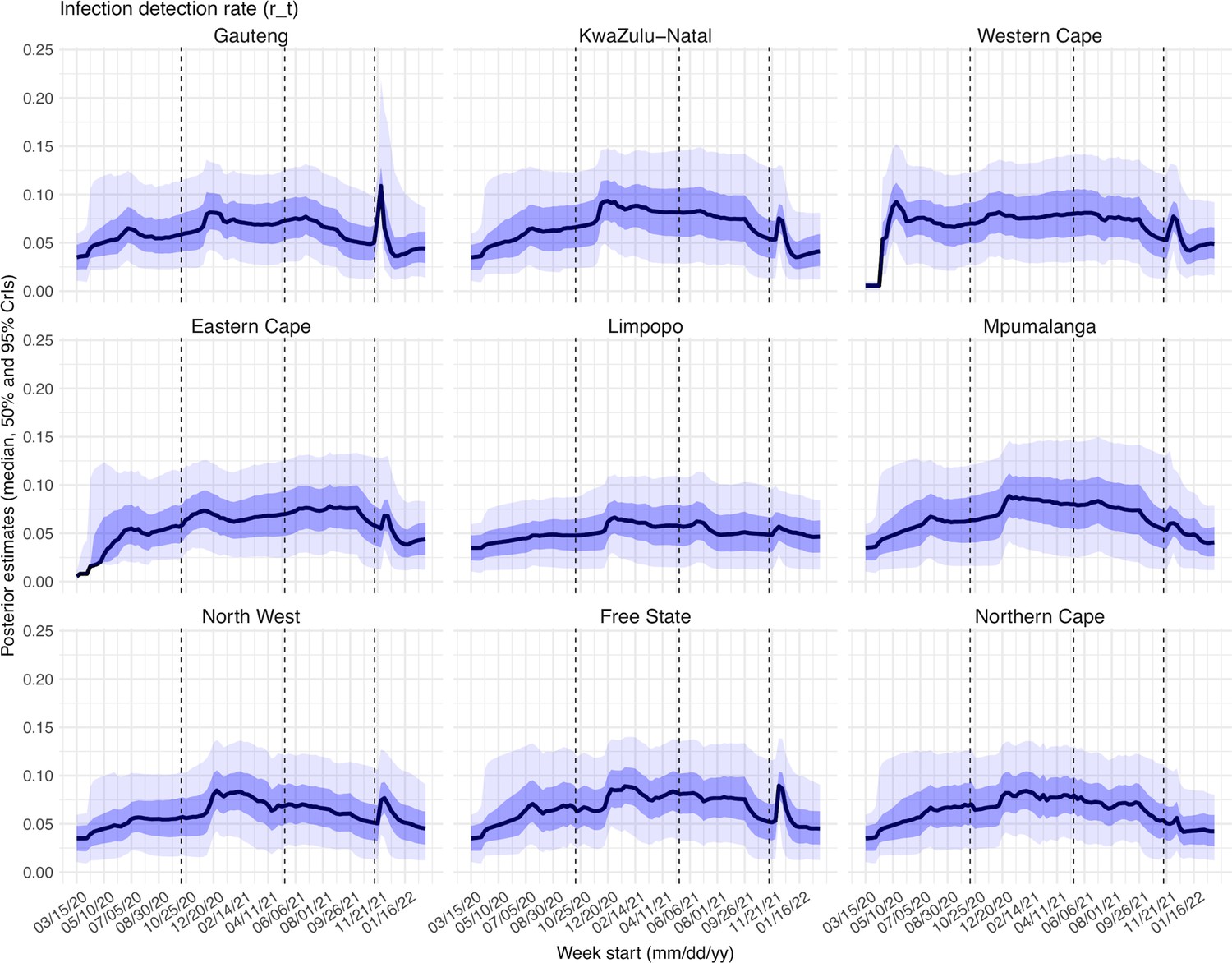
Posterior estimates for infection-detection rate ( in the observation model) by week.
Thick black lines show the median, dark blue areas show the 50% CrIs, and light blue areas show the 95% CrIs. For reference, the dashed vertical black lines indicate three dates (mm/dd/yy), i.e., 10/15/20, 5/15/21, and 11/15/21, roughly the start of the Beta, Delta, and Omicron waves, respectively.
Appendix 1—figure 23

Posterior estimates for infection-fatality risk ( in the observation model) by week.
Thick black lines show the median, dark blue areas show the 50% CrIs, and light blue areas show the 95% CrIs. For reference, the dashed vertical black lines indicate three dates (mm/dd/yy), i.e., 10/15/20, 5/15/21, and 11/15/21, roughly the start of the Beta, Delta, and Omicron waves, respectively.
Author response image 1
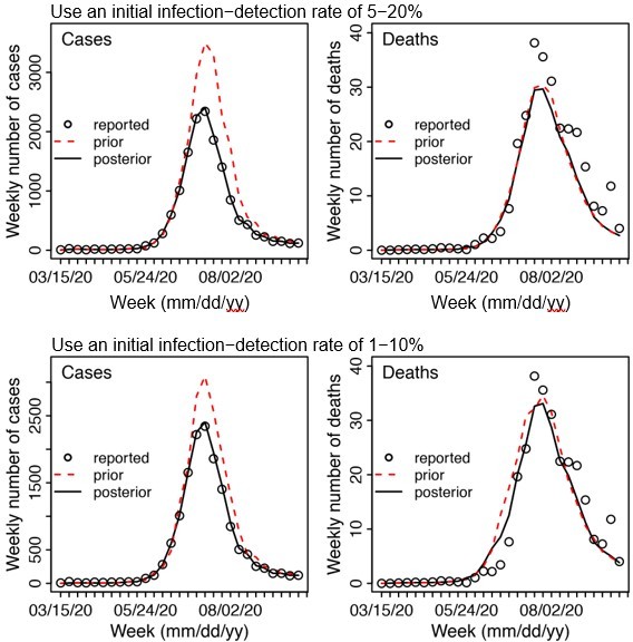
Example test runs comparing initial prior ranges of infection detection rate.
When a higher initial prior range (5 – 20%, top row) was used, the model prior tended to largely over estimate cases and underestimate deaths, suggesting the infection detection rate was likely lower than 5 – 20%; whereas when a lower initial prior range (1-10%, bottom row) was used, the model prior more closely captured the observed weekly cases and deaths throughout the entire first wave, suggesting it is a more appropriate range. Due to the large numbers of parameter range combinations and potential changes over time, we opted to use a wide prior parameter range that is able to reproduce the observed cases and deaths relatively well based on this simple initial test.
Author response image 2
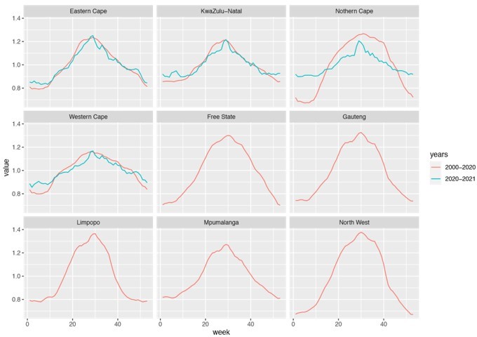
Estimated seasonal trends using climate data during 2000 – 2020 and 2020 – 2021.
Note that data were not available for Free State, Gauteng, Limpopo, Mpumalanga, and North West and only available for 3 weather stations in Northern Cape during years 2020 – 2021.
Tables
Table 1
Estimated increases in transmissibility and immune erosion potential for Beta, Delta, and Omicron (BA.1).
The estimates are expressed in percentage for the median (and 95% CIs). Note that estimated increases in transmissibility for all three variants are relative to the ancestral strain, whereas estimated immune erosion is relative to the composite immunity combining all previous infections and vaccinations accumulated until the surge of the new variant. See main text and Methods for details.
| Province | Quantity | Beta | Delta | Omicron (BA.1) |
|---|---|---|---|---|
| All combined | % Increase in transmissibility | 34.3 (20.5, 48.2) | 47.5 (28.4, 69.4) | 94 (73.5, 121.5) |
| % Immune erosion | 63.4 (45, 77.9) | 24.5 (0, 53.2) | 54.1 (35.8, 70.1) | |
| Gauteng | % Increase in transmissibility | 42.2 (35.6, 48.3) | 51.8 (44.5, 58.7) | 112.6 (96.2, 131.8) |
| % Immune erosion | 65 (57, 72.2) | 44.3 (36.4, 54.9) | 64.1 (56, 74.2) | |
| KwaZulu-Natal | % Increase in transmissibility | 29.7 (22.9, 36.6) | 52.5 (44.8, 60.8) | 90.6 (77.9, 102.4) |
| % Immune erosion | 58.1 (48.3, 71.3) | 17.3 (1.4, 27.6) | 51.1 (39.3, 58.1) | |
| Western Cape | % Increase in transmissibility | 23.4 (20.2, 27.4) | 55.2 (48.2, 62.7) | 86.1 (72.6, 102.6) |
| % Immune erosion | 68.9 (62.5, 76.4) | 41.5 (35.6, 53.5) | 61 (55.5, 67.3) | |
| Eastern Cape | % Increase in transmissibility | 24.1 (18, 29.7) | 50.2 (40.5, 57.4) | 78.4 (67.6, 89.2) |
| % Immune erosion | 54.6 (45.1, 61.2) | 24.2 (15.4, 36.2) | 45.3 (34.5, 57.2) | |
| Limpopo | % Increase in transmissibility | 32.6 (24.9, 39.8) | 38.9 (31.5, 50.5) | 91.8 (82.6, 102.4) |
| % Immune erosion | 56.3 (38.4, 76.2) | 1.8 (0, 21.2) | 42.1 (33.2, 53.2) | |
| Mpumalanga | % Increase in transmissibility | 31.2 (25.4, 38.6) | 35.3 (24.9, 48.2) | 88.6 (72.8, 104.3) |
| % Immune erosion | 55.6 (39.8, 70) | 3.1 (0, 21.7) | 45.9 (37.7, 55.7) | |
| North West | % Increase in transmissibility | 43.8 (36.9, 52.1) | 36.8 (25.6, 47.5) | 100 (81.7, 121.1) |
| % Immune erosion | 67 (58.4, 75.4) | 12.4 (0.4, 30.5) | 56.6 (48.2, 68.8) | |
| Free State | % Increase in transmissibility | 42.7 (35, 49.8) | 43.8 (31.9, 52.1) | 92.2 (77.4, 106.9) |
| % Immune erosion | 70 (64.5, 76.2) | 27.7 (17.6, 41.6) | 57 (49.5, 66.6) | |
| Northern Cape | % Increase in transmissibility | 38.6 (32.6, 44.8) | 63.1 (50.4, 79.2) | 106 (94.7, 119.6) |
| % Immune erosion | 75 (67.4, 82) | 47.9 (40.5, 59.1) | 64 (57.3, 72.6) |
Appendix 1—table 1
Model estimated infection-detection rate during each wave.
Numbers show the estimated percentage of infections (including asymptomatic and subclinical infections) documented as cases (mean and 95% CI in parentheses).
| Province | Ancestral wave | Beta wave | Delta wave | Omicron wave |
|---|---|---|---|---|
| Gauteng | 4.59 (2.62, 9.77) | 6.18 (3.29, 11.11) | 6.27 (3.44, 12.39) | 4.16 (2.46, 9.72) |
| KwaZulu-Natal | 4.33 (2.01, 11.02) | 7.4 (3.89, 13.67) | 5.69 (2.69, 12.34) | 3.25 (1.84, 7.81) |
| Western Cape | 5.62 (3, 10.93) | 7.1 (3.99, 12.78) | 6.83 (3.71, 13.08) | 4.26 (2.49, 9.37) |
| Eastern Cape | 3.79 (1.98, 9.39) | 6.1 (3.35, 11.27) | 5.58 (2.63, 11.52) | 2.91 (1.4, 7.99) |
| Limpopo | 2.13 (0.79, 6.46) | 4.57 (1.89, 10.01) | 3.4 (1.53, 9.3) | 2.9 (1.2, 7.55) |
| Mpumalanga | 3.42 (1.42, 9.1) | 6.28 (2.85, 12.51) | 5.71 (2.58, 12.96) | 3.13 (1.54, 7.24) |
| North West | 3.37 (1.62, 7.88) | 5.79 (2.77, 11.14) | 5.26 (2.8, 10.8) | 3.73 (1.78, 8.62) |
| Free State | 5.02 (2.83, 10.63) | 6.69 (3.69, 11.97) | 6.5 (3.16, 13.23) | 4.03 (2.12, 8.95) |
| Northern Cape | 4.96 (2.75, 10.34) | 6.49 (3.72, 11.44) | 6.69 (3.74, 12.32) | 3.71 (1.97, 8.21) |
Appendix 1—table 2
Model estimated attack rate during each wave.
Numbers show estimated cumulative infection numbers, expressed as percentage of population size (mean and 95% CI in parentheses).
| Province | Ancestral wave | Beta wave | Delta wave | Omicron wave |
|---|---|---|---|---|
| Gauteng | 32.83 (15.42, 57.59) | 21.87 (12.16, 41.13) | 49.82 (25.22, 90.79) | 44.49 (19.01, 75.3) |
| KwaZulu-Natal | 24.06 (9.45, 51.91) | 26.36 (14.28, 50.18) | 27.15 (12.52, 57.39) | 38.11 (15.87, 67.56) |
| Western Cape | 28.44 (14.61, 53.17) | 37.09 (20.61, 66.04) | 47.29 (24.68, 87.1) | 44.1 (20.02, 75.4) |
| Eastern Cape | 32.85 (13.27, 62.95) | 27.44 (14.86, 49.95) | 25.59 (12.4, 54.34) | 26.38 (9.59, 54.69) |
| Limpopo | 13.78 (4.55, 37.21) | 17.12 (7.82, 41.41) | 28.22 (10.33, 62.74) | 18.62 (7.15, 45.01) |
| Mpumalanga | 18.99 (7.14, 45.83) | 17.33 (8.7, 38.21) | 27.18 (11.97, 60.14) | 27.67 (11.96, 56.13) |
| North West | 24.57 (10.51, 51.09) | 16.04 (8.34, 33.49) | 37.21 (18.13, 70.02) | 26.17 (11.33, 54.71) |
| Free State | 39.31 (18.54, 69.57) | 24.23 (13.54, 43.92) | 30.85 (15.16, 63.38) | 32.79 (14.76, 62.32) |
| Northern Cape | 34.92 (16.77, 63.13) | 26.98 (15.3, 47.09) | 55.59 (30.18, 99.32) | 36.87 (16.65, 69.34) |
Appendix 1—table 3
Model estimated infection-fatality risk during each wave.
Numbers are percentages (%; mean and 95% CI in parentheses). Note that these estimates were based on reported COVID-19 deaths and may be biased due to likely under-reporting of COVID-19 deaths. In addition, due to data irregularities, we computed the IFR using two methods. Estimates per Method 1 are the ratio of the total reported COVID-19 related deaths to the model-estimated cumulative infection rate during each wave. Estimates per Method 2 are the weighted average of the weekly IFR estimates during each wave. See details in Section 1 of the Supplemental text.
| Province | Ancestral wave | Beta wave | Delta wave | Omicron wave |
|---|---|---|---|---|
| Estimates per Method 1 (i.e., use reported COVID-19 deaths as the numerator): | ||||
| Gauteng | 0.09 (0.05, 0.2) | 0.19 (0.1, 0.33) | 0.11 (0.06, 0.21) | 0.03 (0.02, 0.06) |
| KwaZulu-Natal | 0.09 (0.04, 0.24) | 0.27 (0.14, 0.49) | 0.14 (0.06, 0.29) | 0.03 (0.02, 0.08) |
| Western Cape | 0.21 (0.11, 0.41) | 0.3 (0.17, 0.54) | 0.25 (0.14, 0.48) | 0.06 (0.04, 0.14) |
| Eastern Cape | 0.11 (0.06, 0.27) | 0.5 (0.27, 0.91) | 0.2 (0.1, 0.42) | 0.08 (0.04, 0.22) |
| Limpopo | 0.06 (0.02, 0.17) | 0.18 (0.08, 0.4) | 0.1 (0.04, 0.27) | 0.05 (0.02, 0.12) |
| Mpumalanga | 0.07 (0.03, 0.18) | 0.1 (0.05, 0.2) | 0.04 (0.02, 0.1) | 0.21 (0.11, 0.5) |
| North West | 0.05 (0.02, 0.11) | 0.21 (0.1, 0.4) | 0.16 (0.08, 0.32) | 0.05 (0.03, 0.12) |
| Free State | 0.13 (0.08, 0.28) | 0.42 (0.23, 0.75) | 0.26 (0.13, 0.52) | 0.09 (0.05, 0.2) |
| Northern Cape | 0.06 (0.03, 0.13) | 0.21 (0.12, 0.37) | 0.17 (0.1, 0.32) | 0.22 (0.12, 0.48) |
| Estimates per Method 2 (i.e., weighted average of weekly IFR estimates): | ||||
| Gauteng | 0.09 (0.02, 0.18) | 0.18 (0.05, 0.38) | 0.12 (0.04, 0.25) | 0.06 (0.01, 0.16) |
| KwaZulu-Natal | 0.16 (0.02, 0.4) | 0.28 (0.07, 0.69) | 0.21 (0.06, 0.55) | 0.08 (0.01, 0.23) |
| Western Cape | 0.23 (0.06, 0.4) | 0.3 (0.11, 0.68) | 0.28 (0.09, 0.56) | 0.13 (0.02, 0.32) |
| Eastern Cape | 0.15 (0.03, 0.33) | 0.39 (0.13, 0.8) | 0.3 (0.07, 0.65) | 0.15 (0.02, 0.39) |
| Limpopo | 0.15 (0.01, 0.31) | 0.19 (0.02, 0.6) | 0.2 (0.03, 0.54) | 0.11 (0.01, 0.31) |
| Mpumalanga | 0.14 (0.01, 0.29) | 0.16 (0.02, 0.39) | 0.1 (0.01, 0.29) | 0.1 (0.01, 0.2) |
| North West | 0.12 (0.01, 0.27) | 0.21 (0.04, 0.45) | 0.17 (0.05, 0.37) | 0.1 (0.01, 0.26) |
| Free State | 0.18 (0.05, 0.45) | 0.46 (0.15, 0.87) | 0.32 (0.09, 0.65) | 0.14 (0.03, 0.34) |
| Northern Cape | 0.12 (0.02, 0.27) | 0.22 (0.07, 0.44) | 0.18 (0.05, 0.34) | 0.1 (0.02, 0.22) |
Appendix 1—table 4
Example estimation of reinfection rates.
As an example, to compute reinfection rates, assume Beta is estimated = 65% immune erosive, Delta is estimated = 40% immune erosive, and Omicron BA.1 is estimated = 65% immune erosive, relative to the combined immunity accumulated until the rise of each of these variants (2nd column); and the attack rates (3rd column) are c1=z1=30%, z2=20%, z3=50%, and z4=40% during the ancestral, Beta, Delta, and Omicron BA.1 waves, respectively. Note these numbers roughly align with our estimates for Gauteng. The cumulative percentage of the population ever infected (including reinfections; 4th column), the percentage of reinfection during each VOC wave among the entire population (5th column) or among those infected by that variant (6th column) can be computed using the approach described in the supplemental text, sub-section “A proposed approach to compute reinfection rates using the model-inference estimates.”
| Variant | Immune erosion, θ | Attack rate, z | Cumulative % ever infected, c | Percentage reinfection this wave, among | |
|---|---|---|---|---|---|
| entire population, η’ | those infected this wave, η | ||||
| Ancestral | - | 30.0% | 30.0% | - | - |
| Beta | 65.0% | 20.0% | 45.6% | 4.4% | 21.8% |
| Delta | 40.0% | 50.0% | 83.1% | 12.6% | 25.1% |
| Omicron (BA.1) | 65.0% | 40.0% | 92.6% | 30.5% | 76.1% |
Appendix 1—table 5
Prior ranges for the parameters used in the model-inference system.
All initial values are drawn from uniform distributions using Latin Hypercube Sampling.
| Parameter/ variable | Symbol | Prior range | Source/rationale |
|---|---|---|---|
| Initial exposed | E(t=0) | 1–500 times of reported cases during the Week of March 15, 2020 for Western Cape and Eastern Cape; 1–10 times of reported cases during the Week of March 15, 2020, for other provinces | Low infection-detection rate in first weeks; earlier and higher case numbers reported in Western Cape and Eastern Cape than other provinces. |
| Initial infectious | I(t=0) | Same as for E(t=0) | |
| Initial susceptible | S(t=0) | 99%–100% of the population | Almost everyone is susceptible initially |
| Population size | N | N/A | Based on population data from COVID19ZA (Data Science for Social Impact Research Group at University of Pretoria, 2021) |
| Variant-specific transmission rate | β | For all provinces, starting from U[0.4, 0.7] at time 0 and allowed to increase over time using space re-probing (Yang and Shaman, 2014) with values drawn from U[0.5, 0.9] during the Beta wave, U[0.7, 1.25] during the Delta wave, and U[0.7, 1.3] during the Omicron wave. | For the initial range at model initialization, based on R0 estimates of around 1.5–4 for SARS-CoV-2. (Li et al., 2020a; Wu et al., 2020; Li et al., 2020b) For the Beta, Delta and Omicron variants, we use large bounds for space re-probing (SR)(Yang and Shaman, 2014) to explore the parameter state space and enable estimation of changes in transmissibility due to the new variants. Note that SR is only applied to 3%–10% of the ensemble members and β can migrate outside either the initial range or the SR ranges during EAKF update. |
| Scaling of effectiveness of NPI | e | [0.5, 1.5], for all provinces | Around 1, with a large bound to be flexible. |
| Latency period | Z | [2, 5] days, for all provinces | Incubation period: 5.2 days (95% CI: 4.1, 7) (Li et al., 2020a); latency period is likely shorter than the incubation period |
| Infectious period | D | [2, 5] days, for all provinces | Time from symptom onset to hospitalization: 3.8 days (95% CI: 0, 12.0) in China, (Zhang et al., 2020) plus 1–2 days viral shedding before symptom onset. We did not distinguish symptomatic/asymptomatic infections. |
| Immunity period | L | [730, 1,095] days, for all provinces | Assuming immunity lasts for 2–3 years |
| Mean of time from viral shedding to diagnosis | Tm | [5, 8] days, for all provinces | From a few days to a week from symptom onset to diagnosis/reporting,(Zhang et al., 2020) plus 1–2 days of viral shedding (being infectious) before symptom onset. |
| Standard deviation (SD) of time from viral shedding to diagnosis | Tsd | [1, 3] days, for all provinces | To allow variation in time to diagnosis/reporting |
| Infection-detection rate | r | Starting from U[0.001, 0.01] at time 0 for Western Cape and Eastern Cape as these two provinces had earlier and higher case numbers during March – April 2020 than other provinces, suggesting lower detection rate at the time; for the rest starting from U[0.01, 0.06]. For all provinces, allowed r to increase over time using space re-probing (Yang and Shaman, 2014) with values drawn from uniform distributions with ranges between roughly 0.01–0.12. | Large uncertainties; therefore, in general we use large prior bounds and large bounds for space re-probing (SR). Note that SR is only applied to 3%–10% of the ensemble members and r can migrate outside either the initial range or the SR ranges during EAKF update. |
| Infection fatality risk (IFR) | For Gauteng: starting from [0.0001, 0.002] at time 0 and allowed to change over time using space re-probing (Yang and Shaman, 2014) with values drawn from U[0.0001, 0.005] during 12/13/2020 – 5/15/21 (due to Beta), U[0.0001, 0.002] during the Delta wave, and U[0.00001, 0.00075] starting 9/1/21 (Omicron wave). For KwaZulu-Natal: starting from U[0.0001, 0.003] at time 0 and allowed to change over time using space re-probing (Yang and Shaman, 2014) with values drawn from U[0.0001, 0.005] during 4/19/20 –10/31/20 (ancestral wave), U[0.0001, 0.01] during 11/1/20 – 5/15/21 (Beta wave), U[0.0001, 0.002] during the Delta wave, and U[0.00001, 0.00075] starting 10/1/21 (Omicron wave). For Western Cape: starting from U[0.00001, 0.003] at time 0 and allowed to change over time using space re-probing (Yang and Shaman, 2014) with values drawn from U[0.00001, 0.0004] during 4/19/20 – 10/31/20 (ancestral wave), U[0.00001, 0.01] during 11/1/20 – 5/15/21 (Beta wave), U[0.00001, 0.005] during 5/16/21 – 9/30/21 (Delta wave) and U[0.00001, 0.002] starting 10/1/21 (Omicron wave). For Eastern Cape: starting from U[0.0001, 0.003] at time 0 and allowed to change over time using space re-probing (Yang and Shaman, 2014) with values drawn from U[0.0001, 0.004] during 4/19/20 – 9/30/20 (Ancestral wave), U[0.0001, 0.01] during 10/1/20 – 40/30/21 (Beta wave), [0.0001, 0.005] during the Delta wave, and U[0.00001, 0.002] or starting 10/16/21 (Omicron wave). For Limpopo and Mpumalanga: starting from U[0.0001, 0.003] at time 0 and allowed to change over time using space re-probing (Yang and Shaman, 2014) with values drawn from U[0.0001, 0.01] during the Beta wave, U[0.0001, 0.005] during the Delta wave, U[0.00001,.002] for the Omicron wave. For Free State: starting from U[0.0001, 0.003] at time 0 and allowed to change over time using space re-probing (Yang and Shaman, 2014) with values drawn from U[0.0001, 0.006] during 3/16/20 – 10/31/20, U[0.0001, 0.01] during the Beta wave, U[0.0001, 0.008] during the Delta wave, and U[0.00001, 0.002] starting 10/1/21 (Omicron wave). For North West and Northern Cape: starting from U[0.0001, 0.003] at time 0 and allowed to change over time using space re-probing (Yang and Shaman, 2014) with values drawn from U[0.0001, 0.005] during the Beta wave, U[0.0001, 0.003] during the Delta wave, and U[0.00001, 0.0015] starting 10/1/21 (Omicron wave). | Based on previous estimates (Verity et al., 2020) but extend to have wider ranges. Note that SR is only applied to 3%–10% of the ensemble members and IFR can migrate outside either the initial range or the SR ranges during EAKF update. Western Cape had earlier and higher case numbers during March – April 2020 than other provinces, suggesting lower detection rate at the time. Initial mortality rate in Gauteng was relatively low because initial infections occurred mainly among middle-aged, returning holiday makers.(Giandhari et al., 2021) Earlier spread of Beta in Eastern Cape, KwaZulu-Natal, and Northern Cape, higher numbers of deaths per capita reported. Free State reported higher number of deaths per capita. |
Appendix 1—table 6
Approximate epidemic timing (mm/dd/yy) for each wave in each province, used in the study.
Note 3/5/22 is the last date of the study period.
| Province | Variant | Start date | End date |
|---|---|---|---|
| Gauteng | Ancestral | 3/15/20 | 10/31/20 |
| Gauteng | Beta | 11/1/20 | 5/15/21 |
| Gauteng | Delta | 5/16/21 | 8/31/21 |
| Gauteng | Omicron | 9/1/21 | 3/5/22 |
| KwaZulu-Natal | Ancestral | 3/15/20 | 9/15/20 |
| KwaZulu-Natal | Beta | 9/16/20 | 5/15/21 |
| KwaZulu-Natal | Delta | 5/16/21 | 9/30/21 |
| KwaZulu-Natal | Omicron | 10/1/21 | 3/5/22 |
| Western Cape | Ancestral | 3/15/20 | 9/15/20 |
| Western Cape | Beta | 9/16/20 | 5/15/21 |
| Western Cape | Delta | 5/16/21 | 9/30/21 |
| Western Cape | Omicron | 10/1/21 | 3/5/22 |
| Eastern Cape | Ancestral | 3/15/20 | 8/15/20 |
| Eastern Cape | Beta | 8/16/20 | 4/30/21 |
| Eastern Cape | Delta | 5/1/21 | 10/15/21 |
| Eastern Cape | Omicron | 10/16/21 | 3/5/22 |
| Limpopo | Ancestral | 3/15/20 | 10/31/20 |
| Limpopo | Beta | 11/1/20 | 5/15/21 |
| Limpopo | Delta | 5/16/21 | 9/30/21 |
| Limpopo | Omicron | 10/1/21 | 3/5/22 |
| Mpumalanga | Ancestral | 3/15/20 | 10/31/20 |
| Mpumalanga | Beta | 11/1/20 | 5/15/21 |
| Mpumalanga | Delta | 5/16/21 | 9/30/21 |
| Mpumalanga | Omicron | 10/1/21 | 3/5/22 |
| North West | Ancestral | 3/15/20 | 10/31/20 |
| North West | Beta | 11/1/20 | 5/15/21 |
| North West | Delta | 5/16/21 | 9/30/21 |
| North West | Omicron | 10/1/21 | 3/5/22 |
| Free State | Ancestral | 3/15/20 | 10/31/20 |
| Free State | Beta | 11/1/20 | 5/31/21 |
| Free State | Delta | 6/1/21 | 9/30/21 |
| Free State | Omicron | 10/1/21 | 3/5/22 |
| Northern Cape | Ancestral | 3/15/20 | 10/31/20 |
| Northern Cape | Beta | 11/1/20 | 5/15/21 |
| Northern Cape | Delta | 5/16/21 | 9/30/21 |
| Northern Cape | Omicron | 10/1/21 | 3/5/22 |
Author response table 1
Raw case fatality ratio (%) by province and pandemic wave.
Raw case fatality ratio is computed as the total number of deaths ÷ total number of cases × 100%.
| Province | Ancestral wave | Β wave | Δ wave | Omicron wave |
|---|---|---|---|---|
| Gauteng | 2.06 | 3 | 1.69 | 0.61 |
| KwaZulu-Natal | 2.15 | 3.6 | 2.39 | 0.99 |
| Western Cape | 3.76 | 4.21 | 3.67 | 1.49 |
| Eastern Cape | 2.92 | 8.11 | 3.65 | 2.8 |
| Limpopo | 2.6 | 4.01 | 2.9 | 1.65 |
| Mpumalanga | 2.03 | 1.62 | 0.77 | 6.85 |
| North West | 1.36 | 3.6 | 2.97 | 1.41 |
| Free State | 2.65 | 6.26 | 3.97 | 2.24 |
| Northern Cape | 1.21 | 3.22 | 2.58 | 5.9 |
Additional files
Download links
A two-part list of links to download the article, or parts of the article, in various formats.
Downloads (link to download the article as PDF)
Open citations (links to open the citations from this article in various online reference manager services)
Cite this article (links to download the citations from this article in formats compatible with various reference manager tools)
COVID-19 pandemic dynamics in South Africa and epidemiological characteristics of three variants of concern (Beta, Delta, and Omicron)
eLife 11:e78933.
https://doi.org/10.7554/eLife.78933


