Figures and data in How enzymatic activity is involved in chromatin organization

Figures
Tables
Additional files

5 figures, 1 table and 3 additional files

Figures

Figure 1

Download asset Open asset

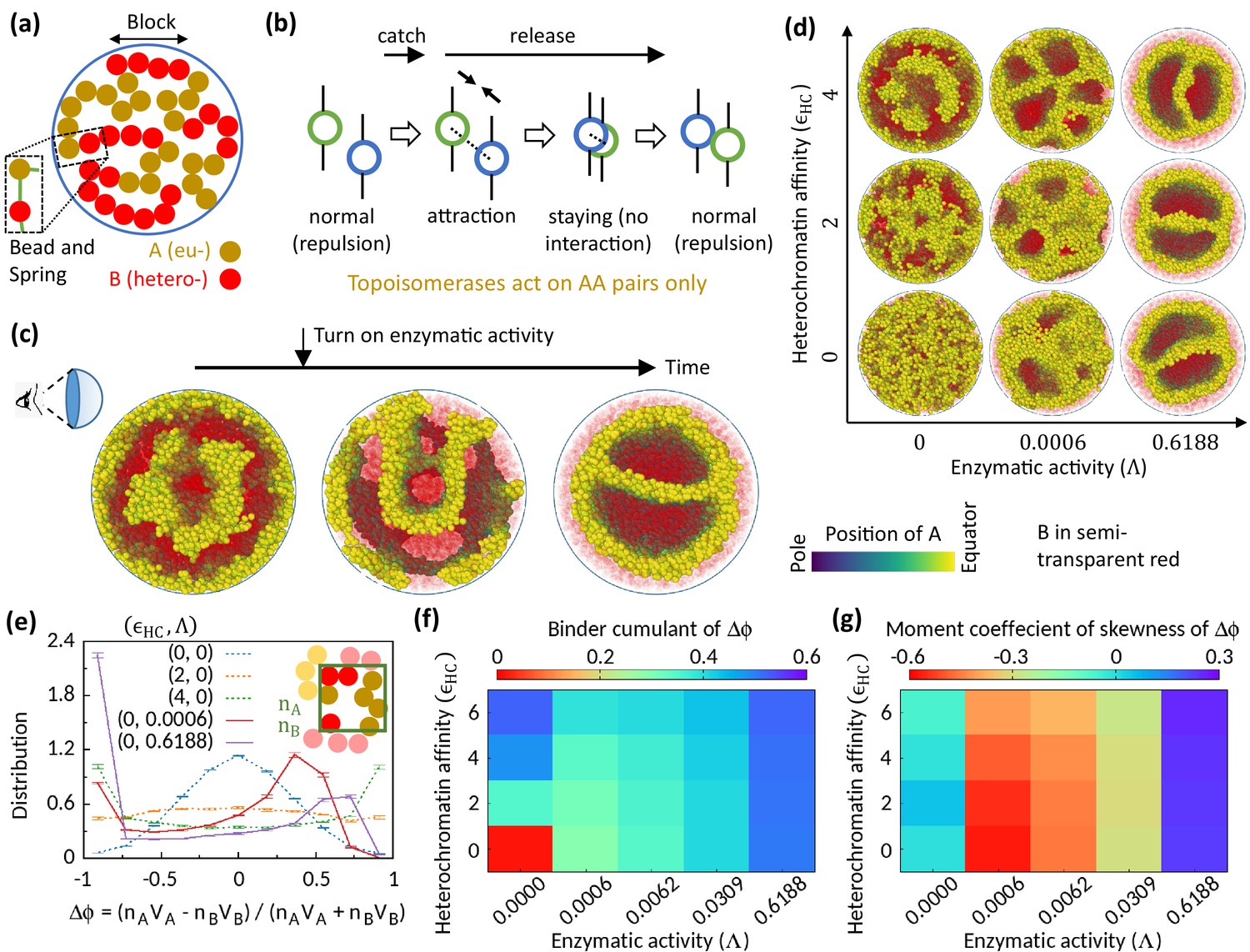
Microphase separation of eu- and heterochromatic regions due to enzymatic activity.

(a) A random multiblock copolymer comprising A and B beads connected by springs confined within a spherical cavity. All the data are shown for block size $b = 4$ . (b) Topo-II enzyme catches two A’s in spatial neighborhood. Through a sequence of processes, it passes one A across another with some probability and eventually releases both A’s. (c) Sample snapshots (hemisphere cuts) showing that microphase separation configuration changes significantly after turning on enzymatic activity. The color bar indicates position of A’s, and B’s are shown in semi-transparent red. Parameters used— $ϵ_{H C} = 4$ and $Λ = 0.6188$ . (d) Sample snapshots showing microphase separation in response to heterochromatin affinity and enzymatic activity. (e) Inset—The cavity is divided into small grids, and $n_{A}$ and $n_{B}$ stand for the numbers of the respective beads within individual grid. Main— $V_{A, B}$ represent volume of the respective beads. Distribution of $Δ ϕ$ goes from unimodal to bimodal as the system phase separates. Time-averaged data shown, and error bars indicate standard deviations over four realizations. (f) Binder cumulant $1 - {⟨ {(Δ ϕ)}^{4} ⟩}_{P} / 3 {⟨ {(Δ ϕ)}^{2} ⟩}_{P}^{2}$ value greater than zero indicates deviation of the $Δ ϕ$ -distribution from the Gaussian profile. (g) Moment coefficient of skewness $E [{(Δ ϕ - ⟨ Δ ϕ ⟩)}^{3}] / {E [{(Δ ϕ - ⟨ Δ ϕ ⟩)}^{2}]}^{3 / 2}$ captures the asymmetry in the $Δ ϕ$ -distribution about its mean in the presence of Topo-II.

Figure 2

Download asset Open asset

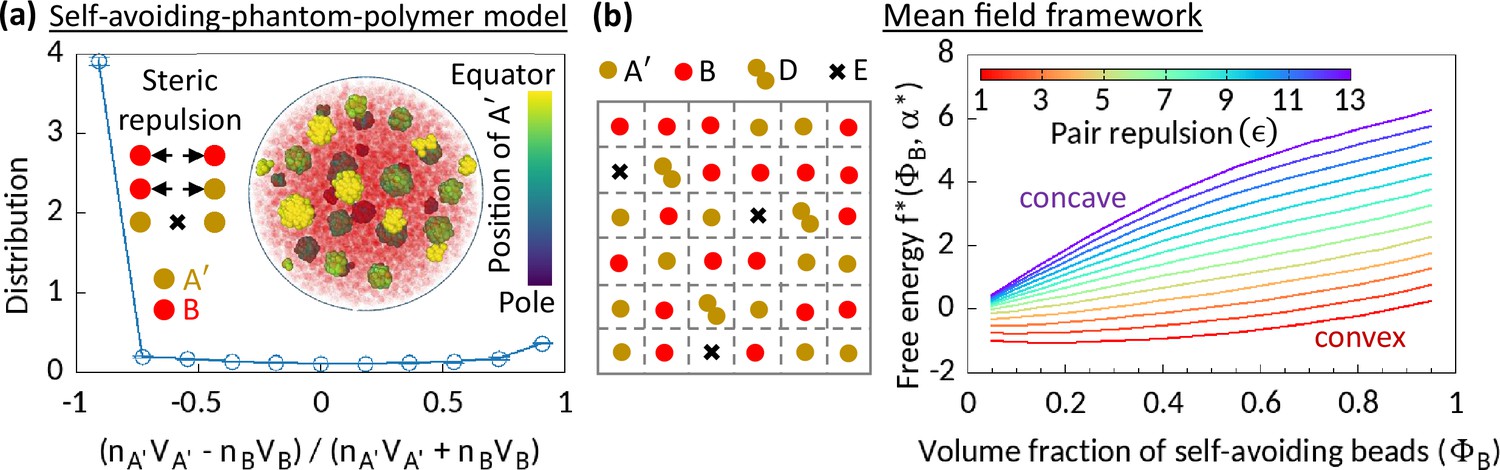
Phase separation in system comprising self-avoiding and phantom regions.

(a) An equilibrium copolymer system comprising phantom (A′) and self-avoiding (B) beads is simulated in the absence of steric interaction between A′’s. The system shows microphase separation. A sample snapshot (hemisphere cut) is shown where B’s are in semi-transparent red. Time-averaged data shown for the distribution, and error bars indicate standard deviations over five realizations. (b) Left—Schematic of a lattice space filled with phantom (A′) and self-avoiding (B) beads. A′ beads can form doublets (D) resulting empty (E) sites. Mean-field calculation gives an effective attraction among B’s. Right—Free energy $f^{*}$ curves drawn for critical doublet fraction $α^{*} (Φ_{B}, ϵ)$ shows convex to concave transition with pair repulsion parameter $ϵ$ , suggesting a phase separation in the system.

Figure 3 with 6 supplements

Download asset Open asset

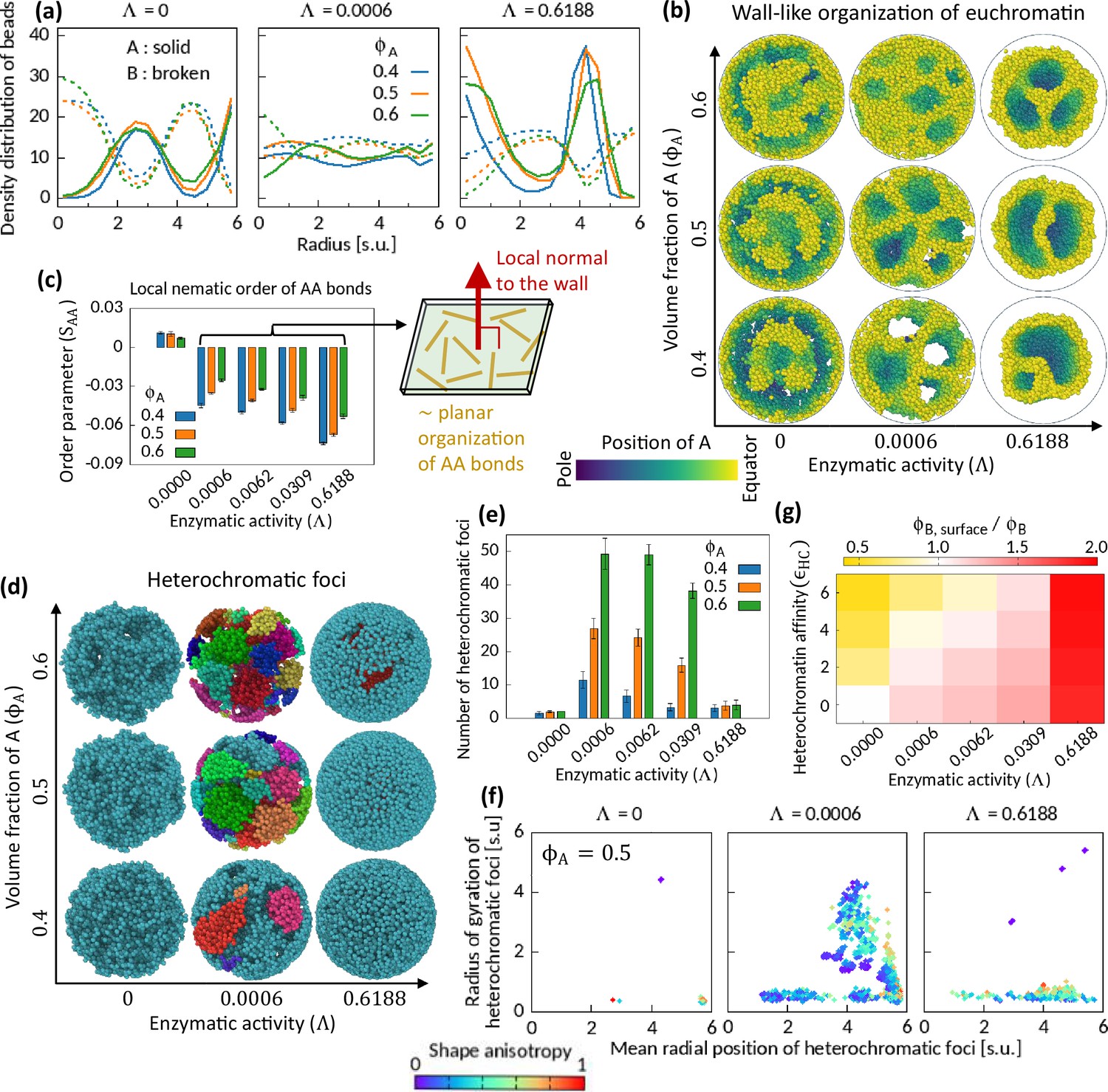
Characteristics of Topo-II-induced microphase separation configurations.

(a) Density distribution of A and B beads in radial direction, plotted for fixed $ϵ_{H C} = 4$ . (b) Sample snapshots (hemisphere cuts) showing wall-like organization of A’s for $Λ > 0$ . (c) Local nematic order parameter of AA bonds. Schematic shows approximate organization of AA bonds in the wall. (**d–f**) Heterochromatic foci features. Sample snapshots (d) and number (e) of heterochromatic foci are shown. In (d), B beads (heterochromatin) are shown, where different color of the beads indicates distinct focus. Time-averaged data are shown in (e) and the error bars indicate standard deviations over four realizations. (f) Position and size of individual focus are respectively represented by the mean radial coordinates of the member-B’s and the radius of gyration of the focus. Shape anisotropy ranges from zero to unity for spherical and line-shaped foci, respectively. (g) Volume fraction of B’s at the surface over the global volume fraction of B is shown in $Λ - ϵ_{H C}$ space for $ϕ_{A} = 0.5$ . Time-averaged data are shown.

Figure 3—figure supplement 1

Download asset Open asset

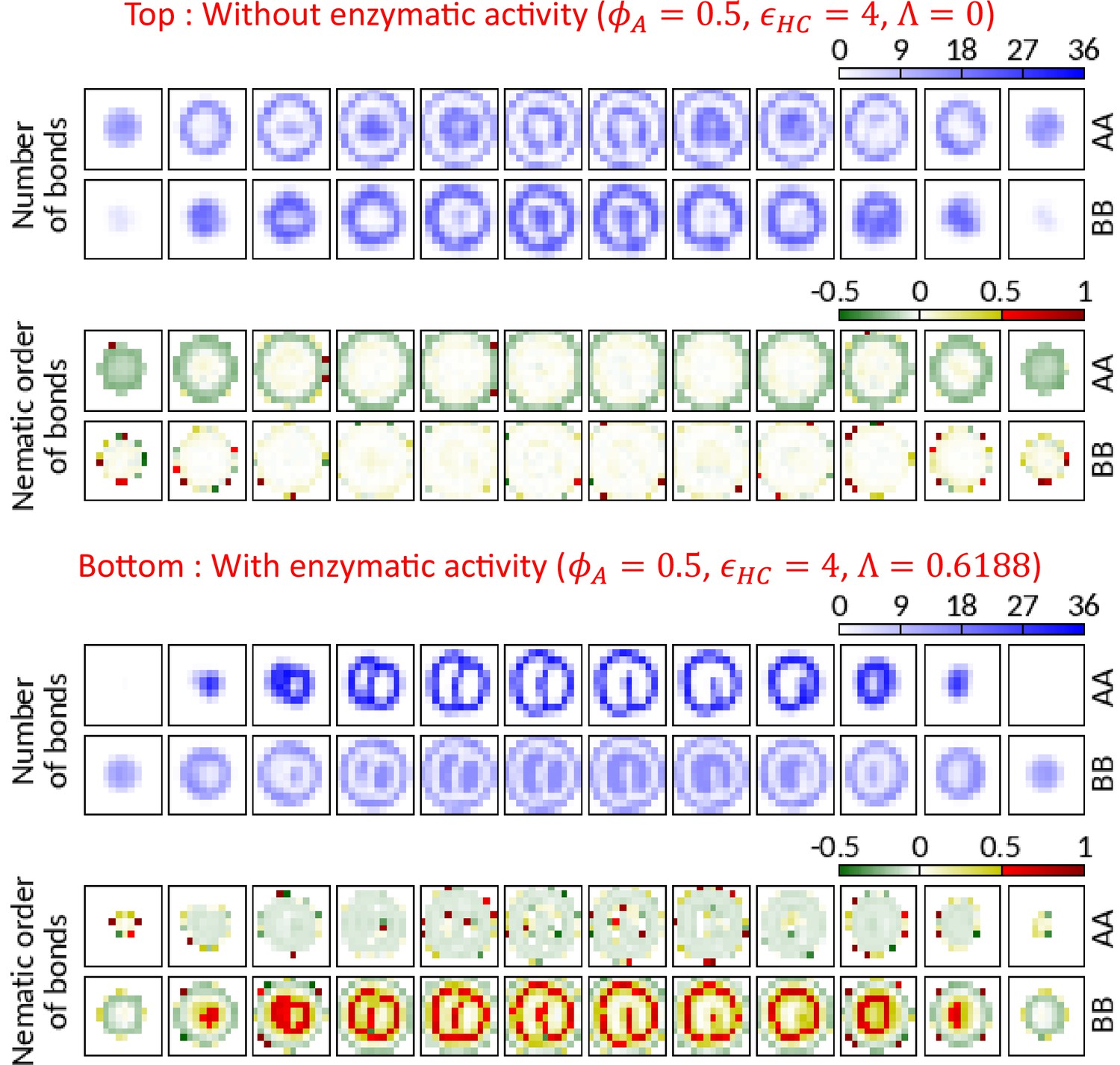
AA bonds along the polymer are organized in planes of the walls formed by Topo-II.

We count the average number of AA and BB bonds (springs) along the polymer in local grids ( $ℓ \times ℓ \times ℓ$ in size) and calculate the amplitude of the nematic order parameter of those bonds. Negative, zero, and positive order parameter values respectively imply planar ordering normal to the director, no ordering, and an ordering parallel to the director. Horizontally arranged 12 boxes represent 12 slices (thickness $ℓ$ ) of the cavity. Top—In the absence of the enzymatic activity, no significant ordering is observed except (i) for AA bonds near the surface due to confinement constraint and (ii) in the grids where there are insufficient number of bonds to calculate order parameter. Bottom—Due to the activity of Topo-II, A beads form wall (refer to the grids with high number of AA bonds) where the amplitude of the order parameter is negative. This suggests that the AA bonds along the polymer are organized in the plane of the wall with local directors normal to the wall (see the schematic in Figure 3c). BB bonds show positive nematic ordering in the presence of enzymatic activity.

Figure 3—figure supplement 2

Download asset Open asset

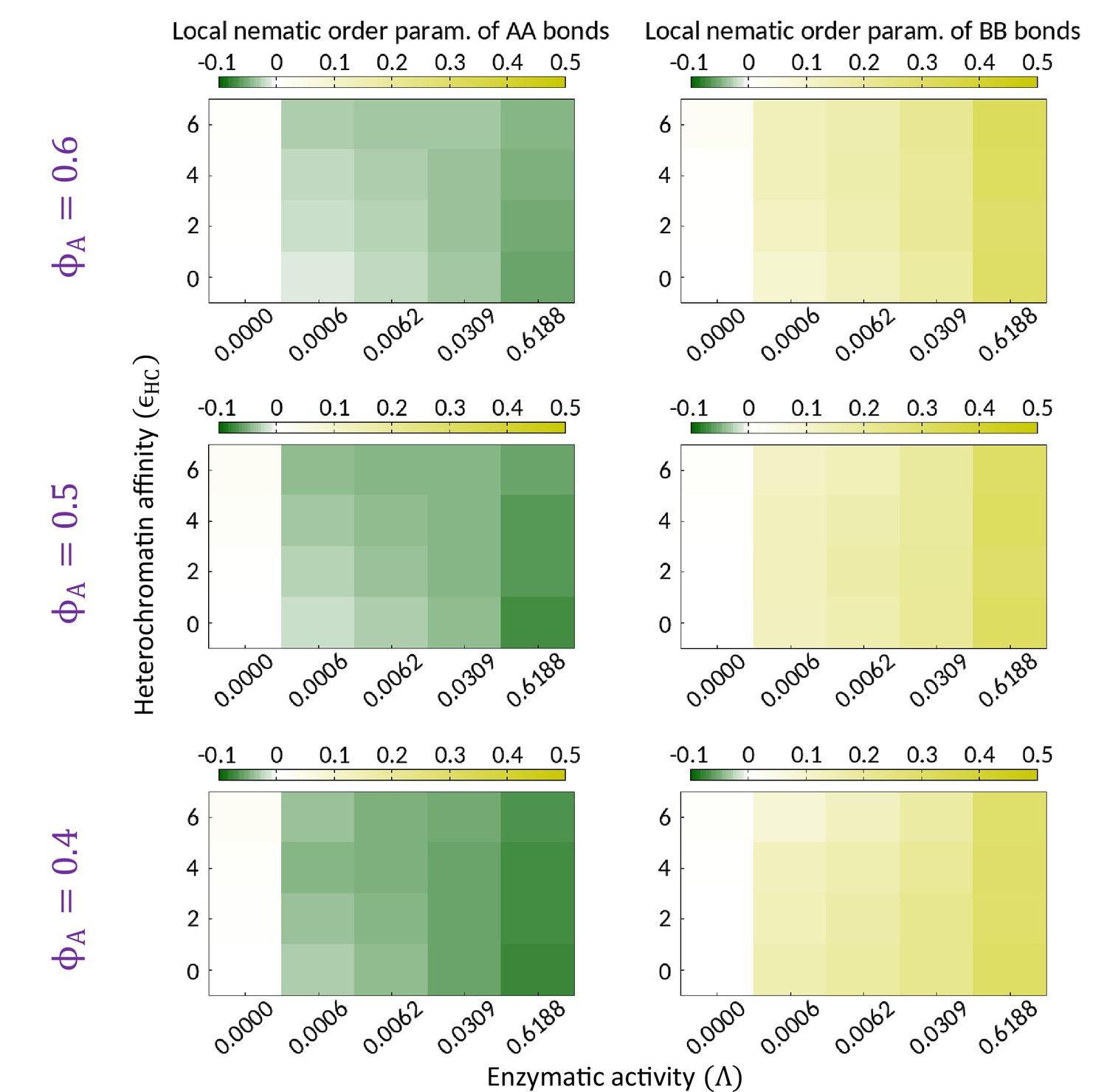
Topo-II breaks local isotropy of the AA and BB bonds.

Phase diagrams indicating the mean local nematic order parameter of the AA and BB bonds (i.e., $S_{A A}$ and $S_{B B}$ ) are shown on the $Λ$ - $ϵ_{H C}$ plane for different composition of the system. $S_{A A} < 0$ and $S_{B B} > 0$ for $Λ > 0$ while both are zero in the absence of the enzymatic activity. The data shown for each parameter set $(ϕ_{A}, Λ, ϵ_{H C})$ is obtained by averaging over several thousand snapshots of single realization.

Figure 3—figure supplement 3

Download asset Open asset

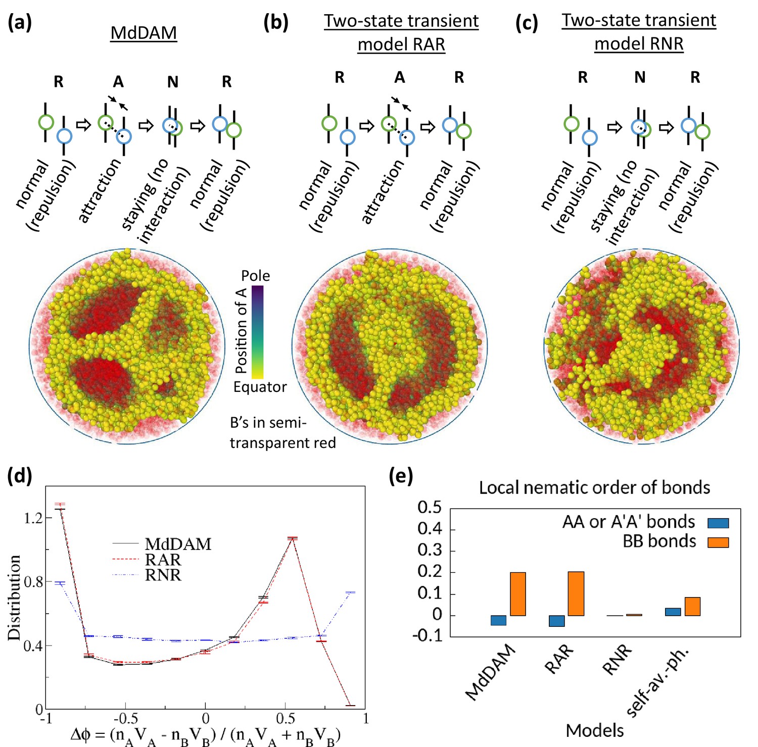
Comparison of monodisperse differential active model (MdDAM) with other transient models.

(a) Model schematic of Topo-II’s activity, and a sample snapshot is shown for $Λ = λ_{r a} (1 / λ_{a n} + 1 / λ_{n r}) = 0.0309$ in the absence of heterochromatin affinity. (**b–c**) Model schematics and sample snapshots are shown for two-state transient models, RAR and RNR. In each of these two models, the rate for switching from repulsion state to the middle state is considered equal to $λ_{r a}$ , and the switching rate from that middle state to the repulsion state is chosen ${(1 / λ_{a n} + 1 / λ_{n r})}^{- 1}$ . This yields activity-like parameter of these two models comparable to the chosen $Λ$ . (d) Time-averaged $Δ ϕ$ -distributions are shown for MdDAM, RAR, and RNR models, obtained from one realization only. The error bars indicate standard deviation over time. (e) Mean local nematic order parameters, $S_{A A}$ and $S_{B B}$ , are shown for different transient models.

Figure 3—figure supplement 4

Download asset Open asset

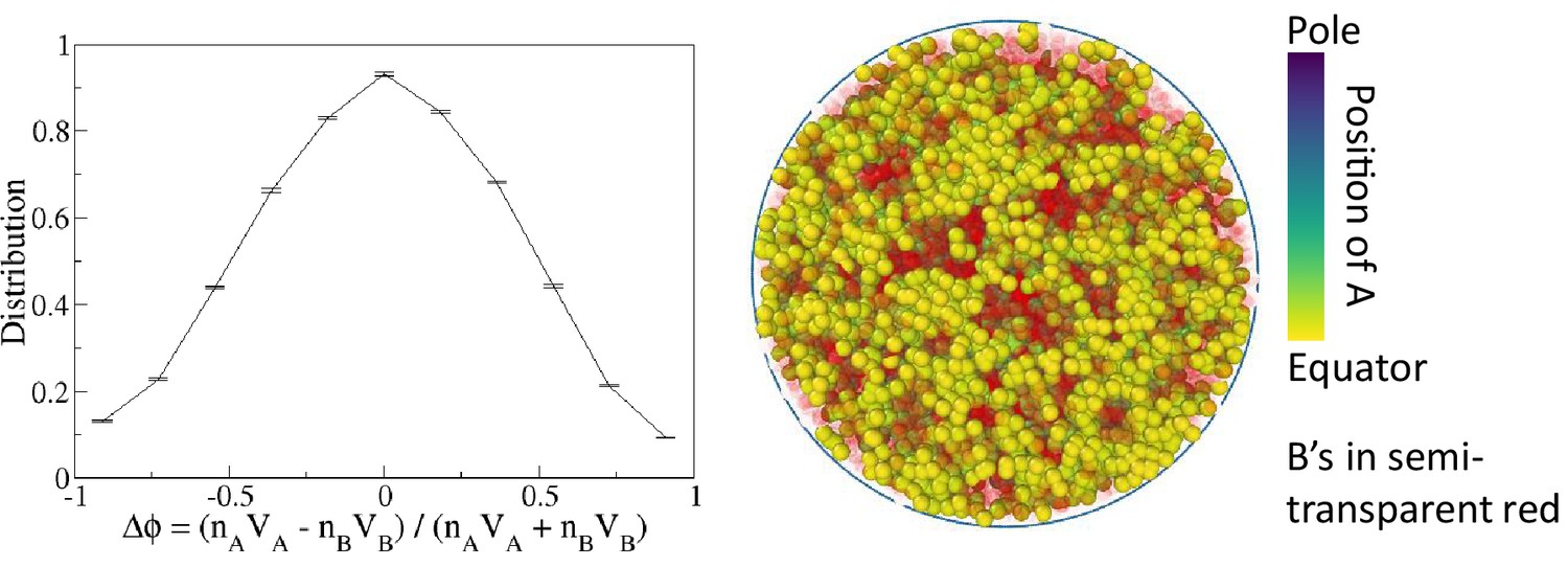
A non-transient effective attraction model comparable to monodisperse differential active model (MdDAM) does not show phase separation.

To construct the effective model, we consider an additional potential $H_{A A} = \sum_{i, j \in A; r_{i j} \leq ℓ} h_{A A} = \sum_{i, j \in A; r_{i j} \leq ℓ} - ϵ_{A A} \exp (- α_{v e x} r_{i j}^{2})$ in Equation 2, and maintain all $h_{v e x}$ ’s in the repulsion state. MdDAM shows strong phase separation for the case with $ϕ_{A} = 0.5$ , $ϵ_{H C} = 0$ , and $Λ = 0.0309$ . For that case, we estimate $ϵ_{A A} ≃ ϵ_{v e x} \times t_{A} / t_{R}$ = 0.24 s.u., where $t_{A} = 1 / λ_{a n}$ and $t_{R} = 1 / λ_{r a}$ are, respectively, times that a pair of A beads on average spends in the attraction state and the repulsion state in MdDAM. The sample snapshot and the order parameter distribution indicate no phase separation in that non-transient effective model.

Figure 3—figure supplement 5

Download asset Open asset

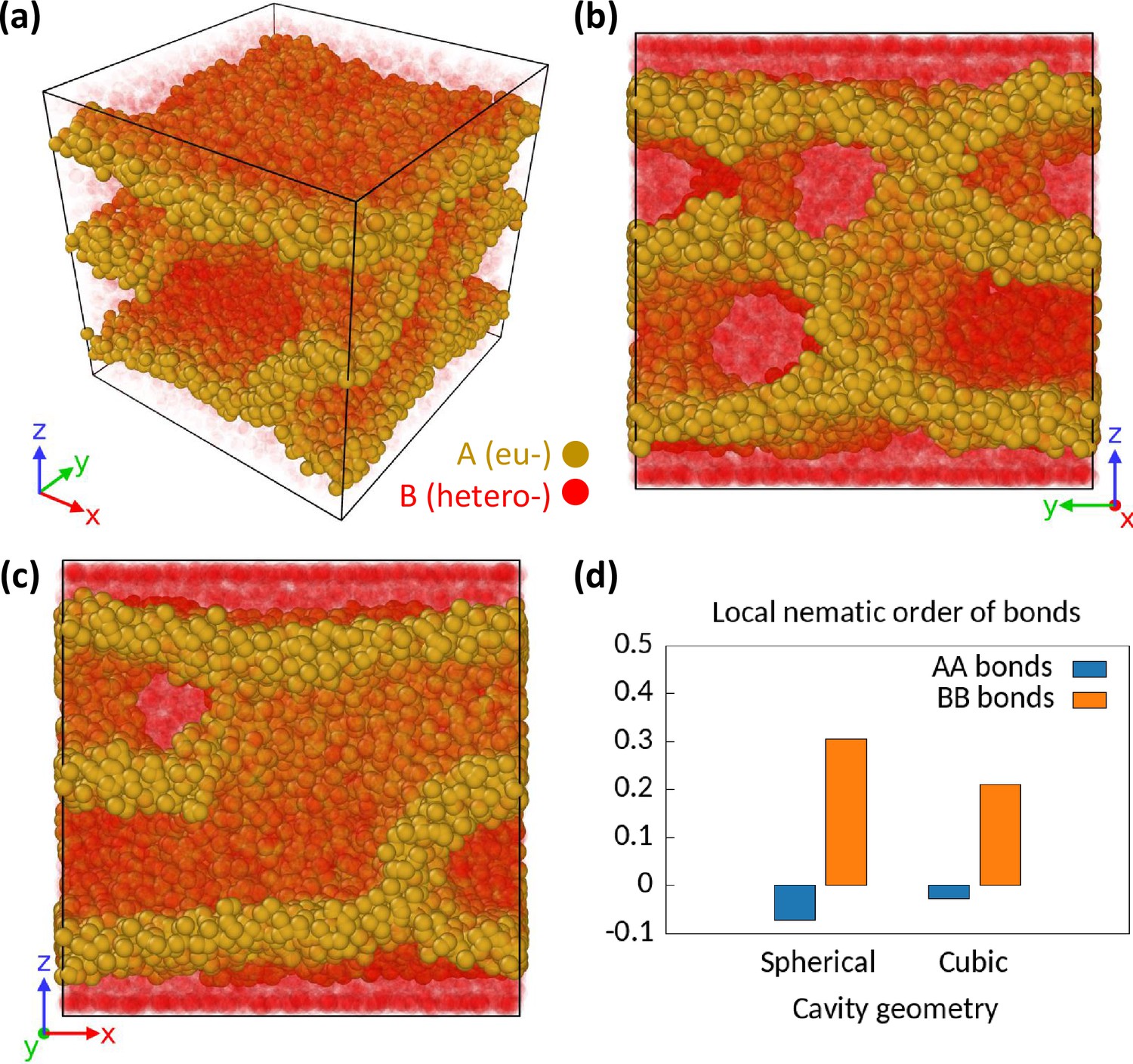
Effect of the geometry of the cavity on phase separation configurations.

We consider a cubic cavity of linear dimension $10 ℓ$ with closed boundary on z-direction. We assume periodic boundary condition for other two directions. We simulate monodisperse differential active model (MdDAM) (polymer length $N = 20992$ ) inside this cubic cavity for $ϕ_{A} = 0.5, Λ = 0.6188,$ and $ϵ_{H C} = 0$ . (**a–c**) A sample snapshot is shown from different angles. The B beads are made semi-transparent for better representation of the whole system. The wall-like appearances of the euchromatic (EC) domains are apparent. There are two layers of B beads next to the two closed boundaries next to which walls of A’s appear. (d) Comparison of $S_{A A}$ and $S_{B B}$ between the cubic and the spherical geometries of the cavity. The local isotropy of the AA and the BB bonds in the presence of enzymatic activity are broken in the cubic geometry too.

Figure 3—figure supplement 6

Download asset Open asset

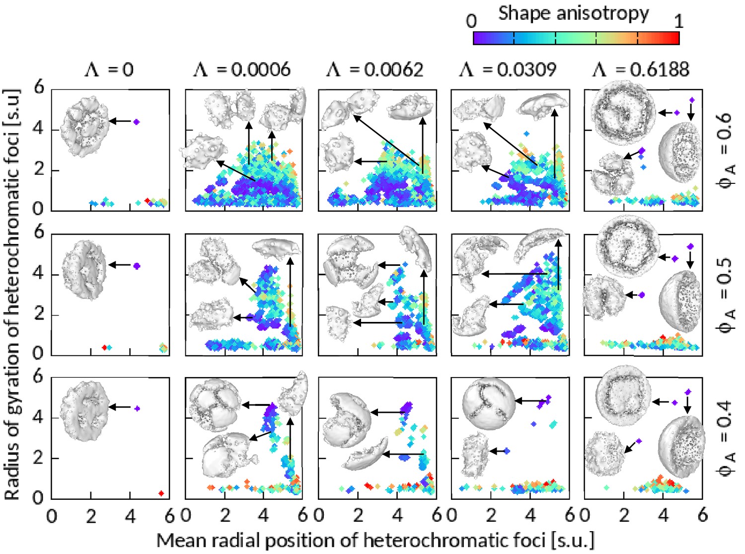
Features of heterochromatic foci shown for $ϵ_{H C} = 4$ .

Radius of gyration of segmented foci are plotted against their mean radial position $r_{f o c i, i} = (\sum_{B \in i} r_{B}) / n_{B, i}$ , $n_{B, i} \equiv$ number of B’s forming foci $i$ . A few sample foci have been shown on the respective panels. The images of the foci are prepared using ‘ambient occlusion’ and ‘construct surface mesh’ modifiers of OVITO. Most of the foci for $Λ = 0$ and 0.6188 are shown in hemisphere-cut view for better presentation.

Figure 4

Download asset Open asset

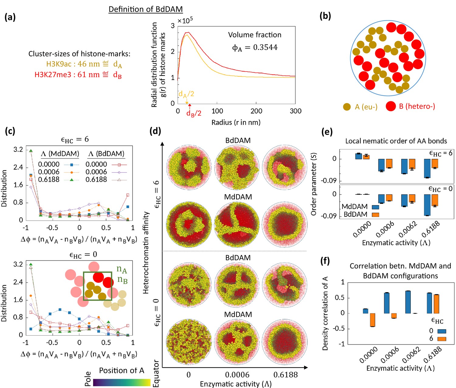
Microphase separation in bidisperse model, motivated from super-resolution microscopy data.

(a) Extracted data for mean cluster sizes and radial distribution functions of histone marks characteristic to eu- and heterochromatic regions. The data were extracted from Xu et al., 2018. Following the experimental data, we set volume fraction $ϕ_{A} = 0.3544$ . (b) Schematic of the bidisperse random multiblock copolymer model. (**c–f**) Comparison of the bidisperse differential active model (BdDAM) with the monodisperse differential active model (MdDAM). Time-averaged $Δ ϕ$ -distributions are shown in (c), and the error bars over realizations are not shown as those are smaller than the symbol sizes. (d) Sample snapshots (hemisphere cuts) are shown, where the B’s are represented in semi-transparent red. The bidisperse system shows phase separation even for $ϵ_{H C} = 0$ and $Λ = 0$ . (e) Local nematic order parameters, averaged over realizations, are shown and the error bars indicate the corresponding standard deviations. (f) Cross-correlation of local density of A’s between MdDAM and BdDAM configurations are shown (see Methods for definition). The data shown are averaged over four realizations, and the error bars indicate the corresponding standard deviations.

Author response image 1

Download asset Open asset

Tables

Table 1

Choice of model parameters.

Potential	Parameters
$H_{s p r i n g}$	$k = 22 e ℓ^{- 2}$ ; $r_{0} = \sum_{i \in c o n n e c t e d b e a d s} d_{i}$ .
$H_{v e x}$	Monodisperse model: $ϵ_{v e x} = 8 e$ ; $α_{v e x} = 7.9585 ℓ^{- 2}$ .
	Bidisperse model for AA pairs: $ϵ_{v e x} = 6.6539 e$ ; $α_{v e x} = 9.5686 ℓ^{- 2}$ .
	Bidisperse model for BB pairs: $ϵ_{v e x} = 11.507 e$ ; $α_{v e x} = 5.5330 ℓ^{- 2}$ .
	Bidisperse model for AB pairs: $ϵ_{v e x} = 8.9153 e$ ; $α_{v e x} = 7.1414 ℓ^{- 2}$ .
$H_{H C}$	$α_{H C} = 100 ℓ^{- 2}$ .
$H_{c o n f i n e m e n t}$	$p = 4 e$ ; $s = 2$ ; $R_{s} = 0.65 R_{g}$ ; $κ = 1 / R_{g}$ ; $R_{g} = d_{i} / 2$ where $i \equiv$ A, B

Additional files

Source code 1 CPU-based FORTRAN simulation code using OpenMP API. Instructions to use this can be found in the README text accompanying the source code.: https://cdn.elifesciences.org/articles/79901/elife-79901-code1-v2.zip
Download elife-79901-code1-v2.zip
Source code 2 CUDA FORTRAN simulation code using GPU acceleration. Instructions to use this can be found in the README text accompanying the source code.: https://cdn.elifesciences.org/articles/79901/elife-79901-code2-v2.zip
Download elife-79901-code2-v2.zip
Transparent reporting form: https://cdn.elifesciences.org/articles/79901/elife-79901-transrepform1-v2.pdf
Download elife-79901-transrepform1-v2.pdf

Download links

A two-part list of links to download the article, or parts of the article, in various formats.

Downloads (link to download the article as PDF)

Open citations (links to open the citations from this article in various online reference manager services)

Mendeley

Cite this article (links to download the citations from this article in formats compatible with various reference manager tools)

Rakesh Das
Takahiro Sakaue
GV Shivashankar
Jacques Prost
Tetsuya Hiraiwa

(2022)

How enzymatic activity is involved in chromatin organization

eLife 11:e79901.

https://doi.org/10.7554/eLife.79901

Share this article

Cite this article

Microphase separation of eu- and heterochromatic regions due to enzymatic activity.

Phase separation in system comprising self-avoiding and phantom regions.

Characteristics of Topo-II-induced microphase separation configurations.

AA bonds along the polymer are organized in planes of the walls formed by Topo-II.

Topo-II breaks local isotropy of the AA and BB bonds.

Comparison of monodisperse differential active model (MdDAM) with other transient models.

A non-transient effective attraction model comparable to monodisperse differential active model (MdDAM) does not show phase separation.

Effect of the geometry of the cavity on phase separation configurations.

Features of heterochromatic foci shown for ϵH⁢C=4.

Microphase separation in bidisperse model, motivated from super-resolution microscopy data.

Choice of model parameters.

Source code 1

Source code 2

Transparent reporting form

Downloads (link to download the article as PDF)

Open citations (links to open the citations from this article in various online reference manager services)

Cite this article (links to download the citations from this article in formats compatible with various reference manager tools)

Features of heterochromatic foci shown for $ϵ_{H C} = 4$ .