Automated systematic evaluation of cryo-EM specimens with SmartScope
- Genome Integrity and Structural Biology Laboratory, National Institute of Environmental Health Sciences, United States
- Department of Computer Science, Duke University, United States
- Department of Electrical and Computer Engineering, Duke University, United States
- Department of Biochemistry, Duke University School of Medicine, United States
Figures
Figure 1 with 3 supplements
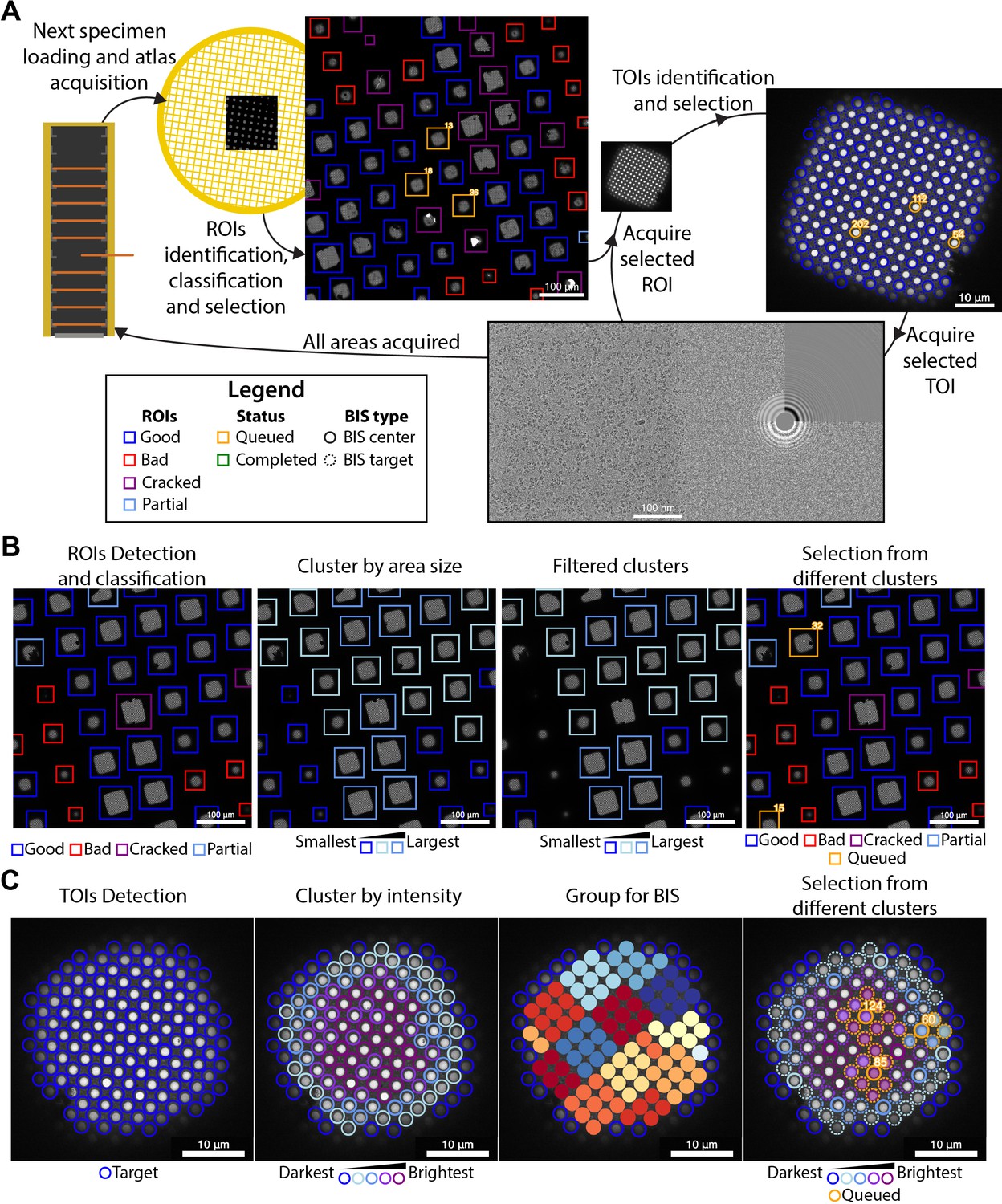
Overview of the SmartScope framework.
(A) Workflow for unsupervised grid navigation and imaging. SmartScope handles specimen exchange, atlas acquisition, regions of interest (ROIs) identification, classification, and selection. It then visits the selected regions and identifies and selects targets of interest (TOIs) which are acquired at higher magnification and preprocessed. (B) Detailed steps in ROI selection. After detection and classification, ROIs are also clustered into groups. In the example is a clustering by size. Then, from the ROIs are queried based on their class and ROIs from different clusters are selected. (C) Detailed steps in TOI selection. Shown here is the hole detection followed by a median intensity clustering. Then, holes are grouped by image-shift radius and groups from each cluster are selected for imaging.
Figure 1—figure supplement 1
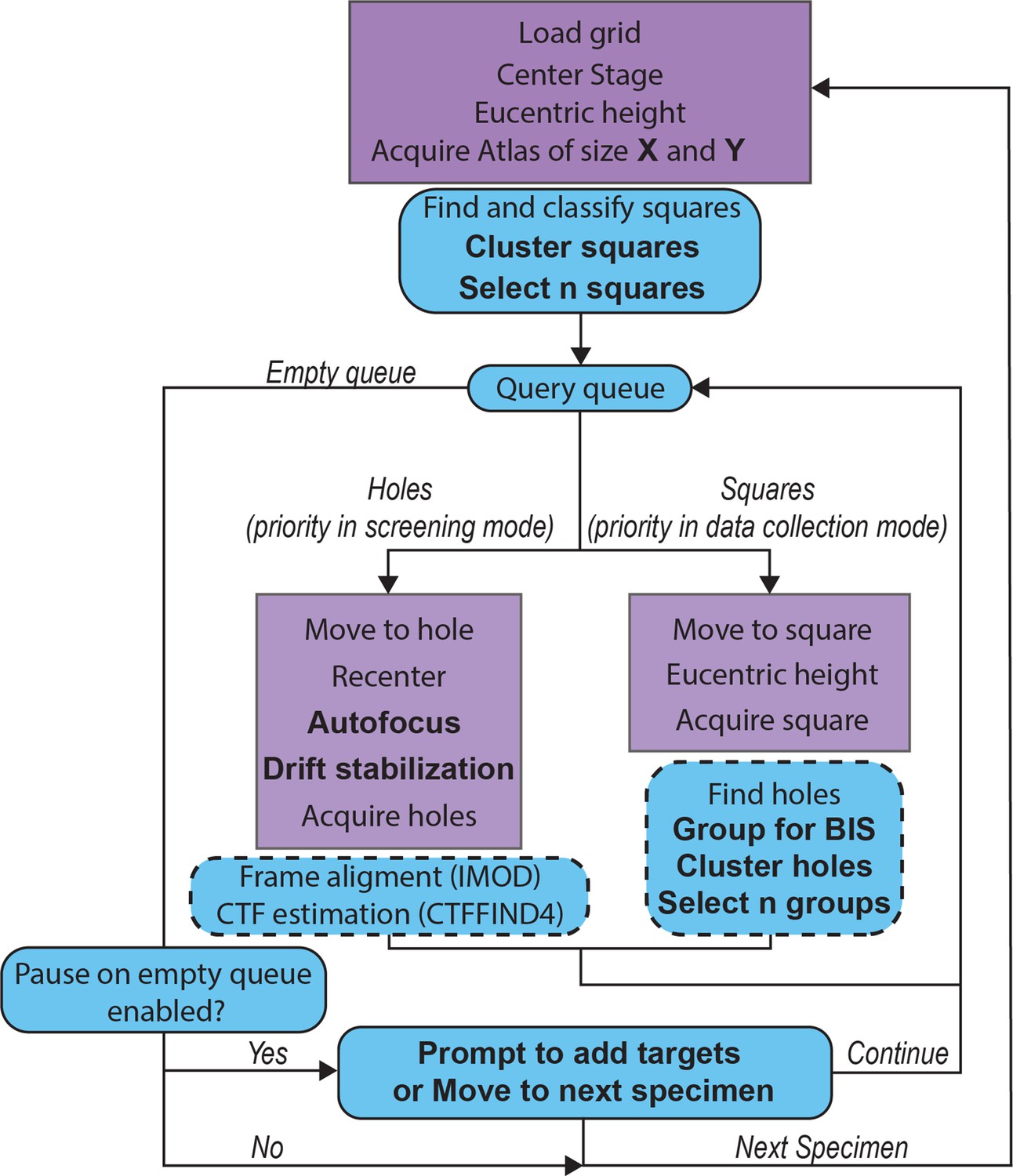
Detailed SmartScope workflow.
Steps carried out by SerialEM (Mastronarde, 2005) are shown in purple and steps carried out by SmartScope are shown in blue. Steps that can be modified within the sessions setup or during the session are shown in bold (see Table 1 for descriptions of the parameters). The steps in the dashed boxes are executed asynchronously from the main workflow, meaning that the workflow moves to the next steps while these are executing.
Figure 1—figure supplement 2
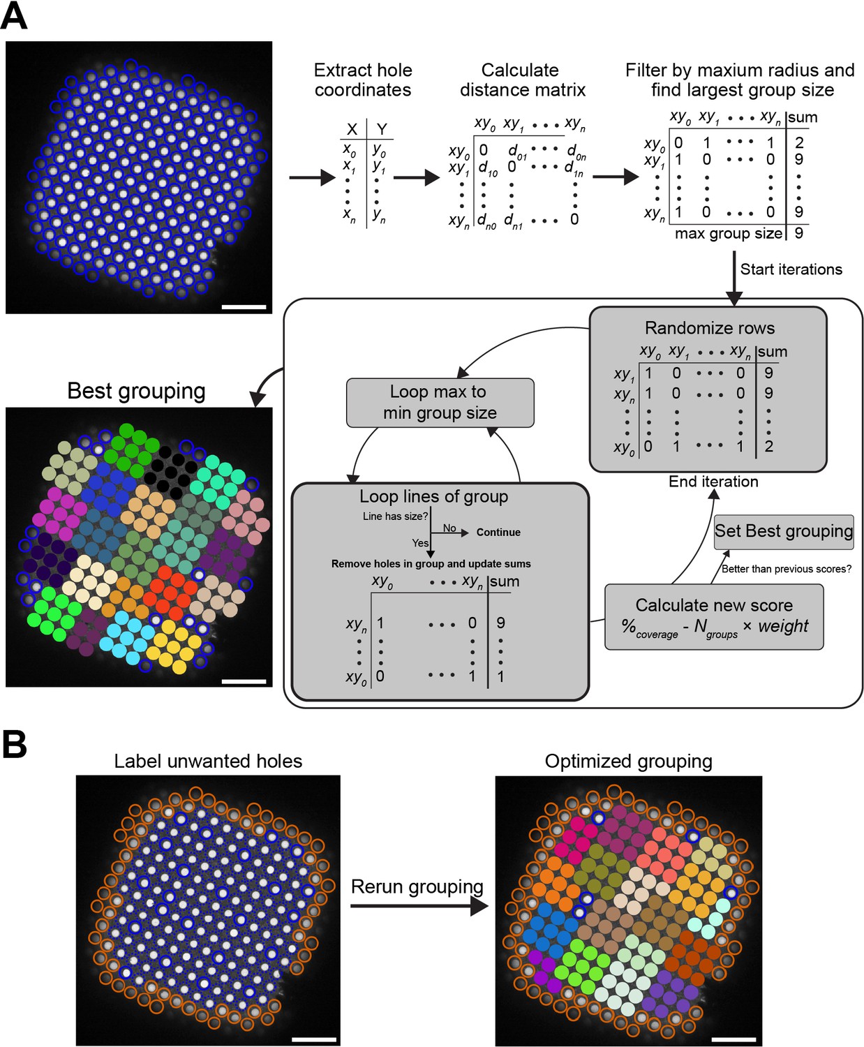
Beam-image shift hole grouping algorithm.
(A) The hole grouping function takes the coordinates of the holes in a square, the maximum grouping radius in microns and a minimum group size. The algorithm uses the distance matrix between the holes and attempts to group them to maximize the coverage while minimizing the number of groups. Each iteration, shown in the dark gray box, uses a randomized matrix. The iterations will stop after 500, unless 250 consecutive iterations did not improve the score. Scores can be weighted in favor of coverage or the number of groups by changing the weight (default weight = 2). (B) Example of how grouping can be optimized by labeling holes bad holes (red) and re-running the grouping algorithm (white scale bars are 10 μm).
Figure 1—figure supplement 3
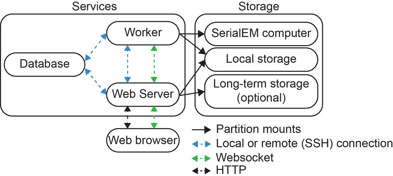
Overall software architecture of SmartScope.
SmartScope uses a database server (MariaDB), a web application with a web server and a Worker that runs the main processes. Each component can be installed on different computers and communicate with each other using Socket or SSH connections. Ongoing sessions are updated in real time via a WebSocket connection. The worker is the only service that requires network access to the SerialEM computer. The worker and Web server need access to a shared disk to continuously update the results. After data is acquired, it can be moved to an optional long-term storage such as a local network drive or to an AWS S3 bucket.
Figure 2 with 1 supplement
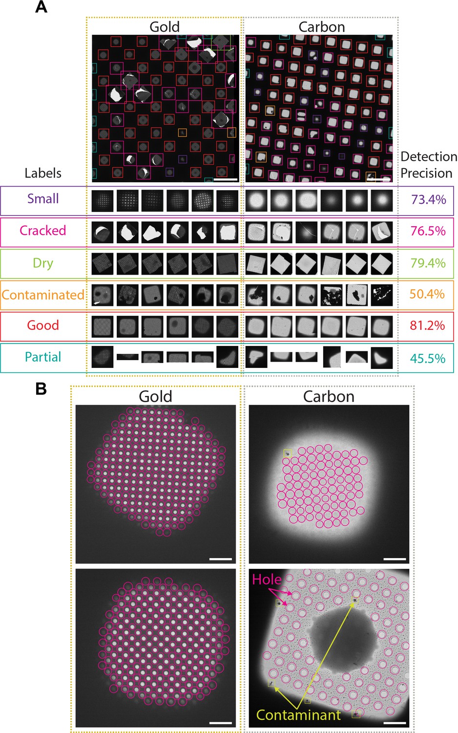
Deep-learning-based feature recognition for autonomous grid navigation.
Sample images show the performance of the square (A) and hole (B) detectors applied to gold (left) and carbon (right) grids. (A) Automatic detection of squares and classification into six different classes: small, cracked, dry, contaminated, good, and partial (white scale bars are 100 μm). Representative examples of squares assigned to each class and corresponding detection precision values are shown (bottom panel). (B) Hole detection performance on representative square images extracted from gold and carbon grids. The hole detector implements a classification step to filter out contaminants (shown in yellow) and increases hole detection precision (shown as pink circles) (white scale bars are 10 μm).
Figure 2—figure supplement 1
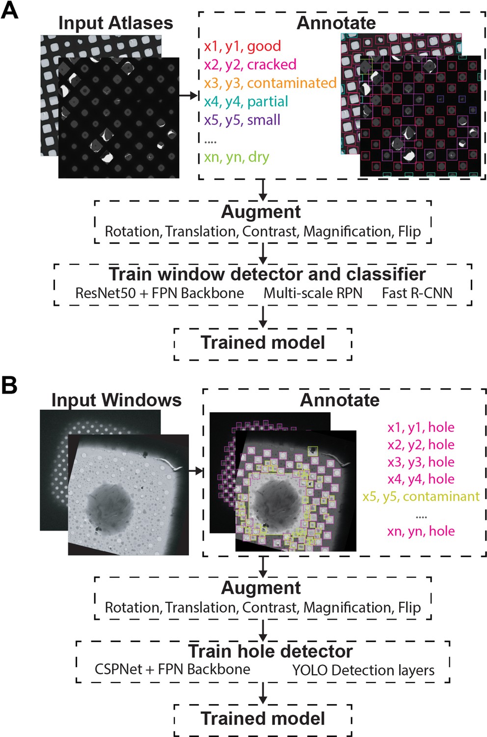
Object detection training strategy.
Atlas (A) and Windows (B) where manually picked and annotated. The annotated dataset was augmented using a combination of rotations, translations, contrast variations, magnifications, and flip transforms. The models were trained against their specific architectures.
Figure 3
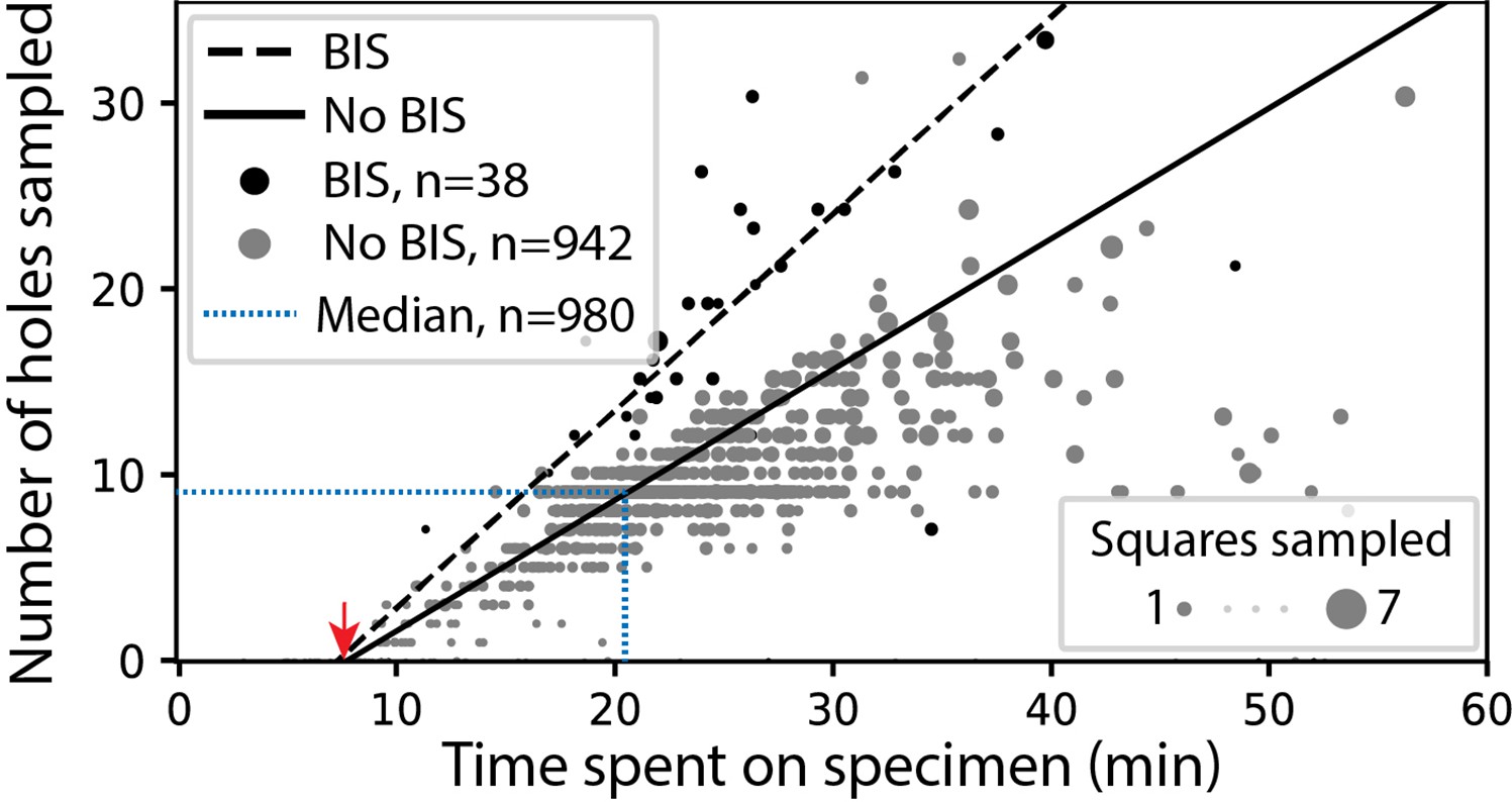
SmartScope’s screening mode statistics.
Screening rates with and without beam-image shift (BIS) were 1.0 and 0.7 holes per minute, respectively (RANSAC regression). The red arrow indicates the time of specimen loading and start of atlas acquisition. Dashed blue line represents the median session duration (21.6min) and the median number of high-magnification images (9.0) obtained per specimen during screening mode.
Figure 4 with 2 supplements
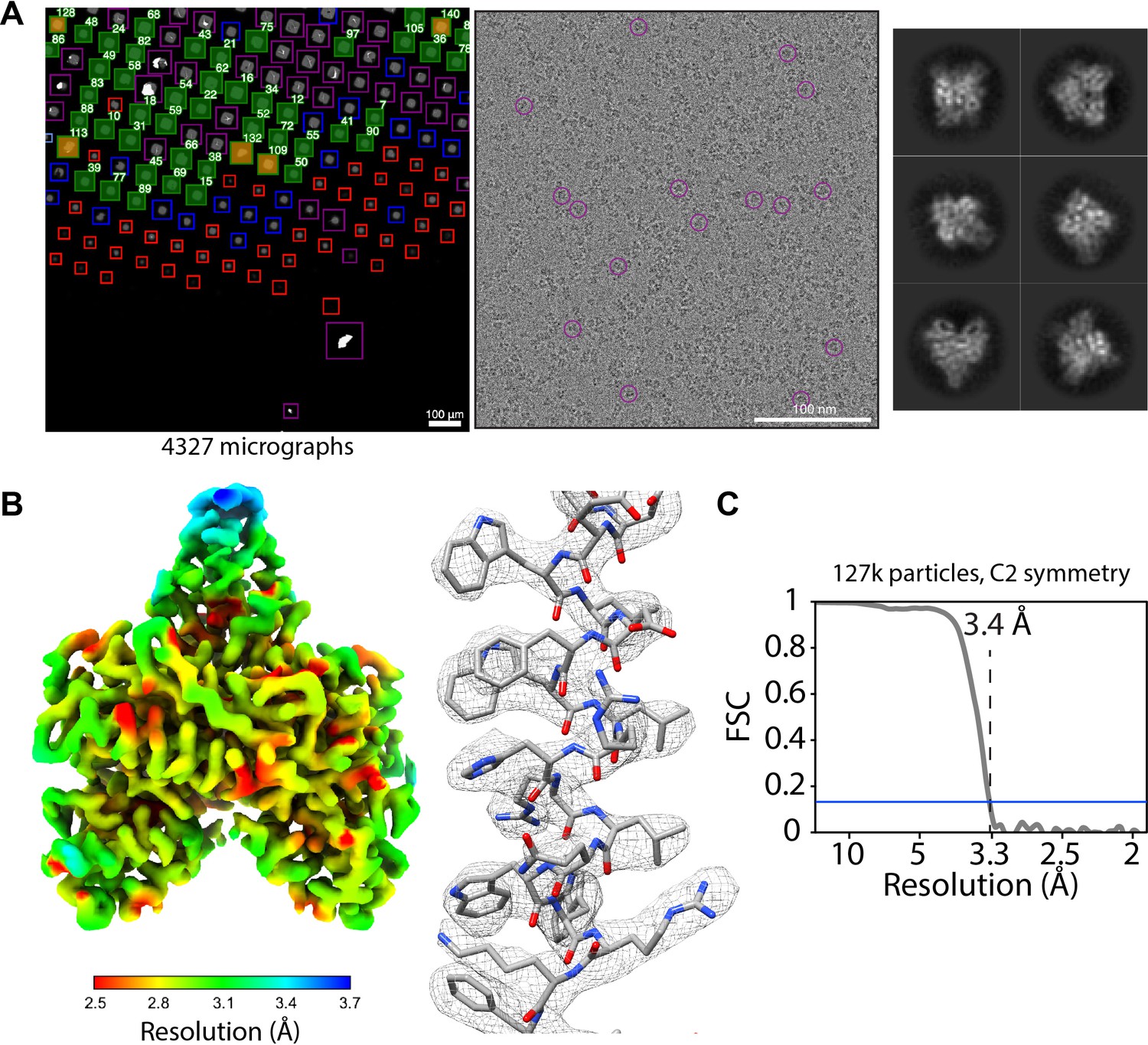
Acquisition of POLG2 dataset using SmartScope.
(A) Atlas of the specimen (left), typical micrograph (center) with some particles picked (purple circles) and 2D classes of POLG2 (right). (B) Resulting map of POLG2 colored by local resolution (left) and example of an alpha helix with atomic model fit into the density (left). (C) Masked Fourier-shell correlation curve between half-maps showing a resolution of 3.4Å.
Figure 4—figure supplement 1
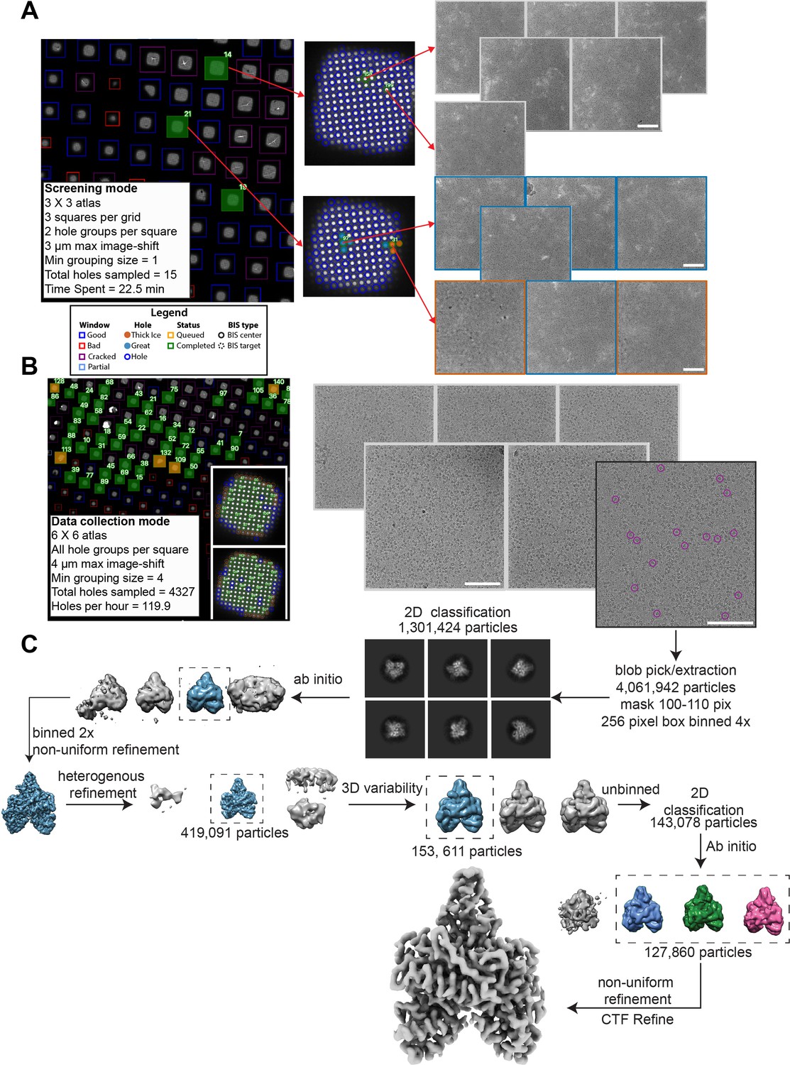
Structure determination of POLG2 using SmartScope.
(A) Screening of the specimen used for POLG2 data collection. Sample images from screening are shown. Data can be labeled from the webUI as a way to keep track of the quality. The holes will be colored according to their quality (red: thick ice, blue: great) (white scale bars are 100 nm). (B) Data collection of the same POLG2 specimen with sample squares and micrographs. Purple circles on the micrographs represent POLG2 particles (right). (C) Data processing of the POLG2 dataset using cryoSPARC (Punjani et al., 2017).
Figure 4—figure supplement 2
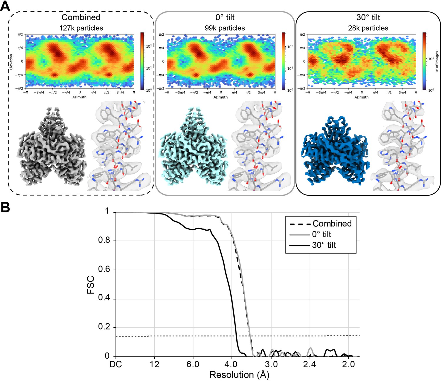
POLG2 particles from the areas collected at 0° tilt, 30° tilt, and combined.
(A) For each set, the angular distribution plot, the map and a zoom into a helix where PDB ID: 2G4C was fitted. All maps are displayed at a contour level of 0.6. (B) FSC plot of each set. Resolutions values can be found in Table 1. The horizontal dashed line represents the 0.143 FSC threshold.
Tables
Table 1
Cryo-EM data acquisition parameters and statistics.
| POLG2 (EMD-25764) | |||
|---|---|---|---|
| No tilt | Tilted | Combined | |
| Hardware | |||
| Microscope | Talos Arctica (Thermo Fisher) | ||
| Detector | K2 summit (Gatan Inc) | ||
| Data collection and processing | |||
| Magnification | 45,000 | ||
| Voltage (kV) | 200 | ||
| Electron exposure (e-/Å2) | 50 | ||
| Defocus range (µm) | 1.2–1.8 | 1.4–1.6 | 1.2–1.8 |
| Tilt angle (°) | 0 | 30 | |
| Pixel size (Å/pixel) | 0.932 | ||
| Movie No. | 3029 (70%) | 1282 (30%) | 4311 |
| Symmetry imposed | C2 | ||
| Final particles | 99,189 (78%) | 28,641 (22%) | 127,860 |
| Map resolution (unmasked) | 3.7 | 4.3 | 3.7 |
| Map resolution (masked) | 3.5 | 3.9 | 3.4 |
| FSC threshold | 0.143 | ||
| Data collection statistics | |||
| Setup time* (min) | 60 | ||
| Throughput (movies/hr) | 117.9 | ||
| Throughput last hour (movies) | 130 | ||
-
*
Data collection times are calculated as the time needed from grid loading to the collection of the first 50 high-magnification targets minus the time required for these 50 targets to be acquired.
Appendix 1—table 1
Input parameters for a SmartScope session.
Parameter names and their description. This is presented as a form on the web interface. These parameters can also be updated during the imaging process.
| Parameter name | Description |
|---|---|
| General session parameters | |
| Session name | Name of the microscopy session |
| Group | Group name of the microscopy session. Usually the principal investigator’s name |
| Microscope | Microscope being used for the session |
| Detector | Detector being used for the session |
| Collection parameters | |
| Atlas X | Number of tiles for the Atlas acquisition in X axis (default: 3) |
| Atlas Y | Number of tiles for the Atlas acquisition in Y axis (default: 3) |
| Square X | Number of tiles for the window acquisition in X axis (default: 1) |
| Square Y | Number of tiles for the window acquisition in the Y axis (default: 1) |
| Squares num | Number of windows to be selected for high-magnification imaging (default: 3) |
| Holes per square | Number of targets per windows to be selected for higher-magnification imaging. If 0 is entered, all targets will be selected and data collection mode will be enabled (default: 3) |
| BIS max distance | Beam-Image shift grouping radius in microns (default: 0) |
| Min BIS group size | Smallest Beam-Image shift group size to be considered (default: 1) |
| Target defocus min | Lower end of the defocus range for rolling defocus in microns (default: –2) |
| Target defocus max | Higher end of the defocus range for rolling defocus in microns (default: –2) |
| Defocus step | Step by which the defocus is varied between each target group (default: 0) |
| Drift crit | Drift threshold to be met during the drift settling procedure before proceeding with high-magnification imaging. Use –1 to disable (default: –1) |
| Tilt angle | Tilt angle to use for high-magnification imaging. Works with BIS enabled (default: 0) |
| Save frames | Whether to save the movie frames or return aligned sum (default: Saving enabled) |
| Zeroloss delay | Time delay in hours for zero loss peak refinement. Only useful if the microscope has an energy filter. Use –1 to deactivate (default: –1) |
| Offset targeting | Enable random targeting off-center to sample the ice gradient and carbon mesh particles. Automatically disabled in data collection mode (default: enabled) |
| Offset distance | Override the random offset by an absolute value in microns. Can be used in data collection mode. Use –1 to disable (default: disabled) |
| Autoloader (1 per grid) | |
| Name | Name of the grid |
| Position | Position in the autoloader |
| Hole type | Grid hole spacing type (i.e. R1.2/1.3) |
| Mesh size | Grid mesh size and spacing (i.e. 300) |
| Mesh material | Grid mesh material (i.e. carbon or gold) |
Appendix 1—table 2
Examples of SerialEM settings for SmartScope usage.
These settings serve as guidelines and will need to be adapted for different hardware combinations. Updated versions of this table can be found at github.com/NIEHS/SmartScope.
| Example 1 | Example 2 | |
|---|---|---|
| Instrument | ||
| Microscope | Talos Arctica | Titan Krios G4 |
| Detector | Gatan K2 Summit | Gatan K3 |
| Energy filter | - | Gatan BioContiuum |
| Low Dose Presets | ||
| Search | ||
| Magnification | 210 | 580 |
| Pixel size (Å/pixel) | 196 | 152 |
| Mode | Linear | Counting |
| View | ||
| Magnification | 2600 | 8700 |
| Pixel size (Å/pixel) | 16.1 | 10.1 |
| Mode | Linear | Counting |
| Focus/record | ||
| Magnification* | 36,000 | 81,000 |
| Pixel size (Å/pixel)* | 1.19 | 1.08 |
| Mode | Counting | Counting |
| Full grid montage presets | ||
| Magnification | 62 | 135 |
| Pixel size (Å/pix) | 644 | 654 |
| Mode | Linear | Counting |
-
*
These are the presets that are used for screening. They can be changes to suit the requirement for the specimen.
Appendix 1—table 3
Average precision obtained for each type of grid square.
| Feature type | Small | Cracked | Dry | Contaminated | Good | Partial |
|---|---|---|---|---|---|---|
| Without augmentation | 65.7% | 71.6% | 77.9% | 46.7% | 77.7% | 45.0% |
| With augmentation | 73.4% | 76.5% | 79.4% | 50.41% | 81.2 % | 45.5% |
Appendix 1—table 4
Smartscope screening mode statistics.
All grids were collected using a K2 detector. The default parameters for screening mode are a 9-tile atlas, 3 squares and 3 holes per square.
| Total specimens = 981 | min | max | mean | median | standard deviation |
|---|---|---|---|---|---|
| Squares sampled | 0 | 7 | 2.5 | 3.0 | 1.3 |
| Holes sampled | 0 | 33 | 8.0 | 9.0 | 5.0 |
| Time spent on specimen (min) | 3.0 | 56.3 | 21.0 | 20.9 | 8.4 |
Appendix 1—table 5
Smartscope screening mode statistics excluding specimens with no usable or visible squares.
All grids were collected using a K2 detector. The default parameters for screening mode are a 9-tile atlas, 3 squares and 3 holes per square.
| Total specimens = 772 | min | max | mean | median | standard deviation |
|---|---|---|---|---|---|
| Square sampled | 1 | 7 | 3.0 | 3.0 | 0.9 |
| Hole sampled | 1 | 33 | 9.4 | 9.0 | 4.0 |
| Time spent on specimen (min) | 9.1 | 56.3 | 23.0 | 21.7 | 6.7 |
Appendix 1—table 6
Smartscope data collection mode statistics.
Start times are at the start of specimen loading in the column. All grids were imaged using a K2 detector.
| Total specimens = 58 | min | max | median | mean ± SD |
|---|---|---|---|---|
| Total micrographs | 565 | 8333 | 1626 | 2155±1502 |
| Holes per hour | 51 | 141 | 100 | 100±22 |
| Data collection setup time (min)* | 6 | 80 | 32 | 34±17 |
| Setup time per 1000 micrographs (min) | 4 | 55 | 17 | 19±11 |
-
*
Data collection times are calculated as the time needed from grid loading to the collection of the first 50 high-magnification targets minus the time required for these 50 targets to be acquired.
Additional files
Download links
A two-part list of links to download the article, or parts of the article, in various formats.
Downloads (link to download the article as PDF)
Open citations (links to open the citations from this article in various online reference manager services)
Cite this article (links to download the citations from this article in formats compatible with various reference manager tools)
Automated systematic evaluation of cryo-EM specimens with SmartScope
eLife 11:e80047.
https://doi.org/10.7554/eLife.80047


