A generalizable brain extraction net (BEN) for multimodal MRI data from rodents, nonhuman primates, and humans
- Institute of Science and Technology for Brain-Inspired Intelligence, Fudan University, China
- MOE Key Laboratory of Computational Neuroscience and Brain-Inspired Intelligence, Fudan University, China
- MOE Frontiers Center for Brain Science, Fudan University, China
- Institute of AI for Health (AIH), Helmholtz Zentrum München, Germany
- School of Biomedical Engineering, ShanghaiTech University, China
- Shanghai United Imaging Intelligence Co., Ltd, China
- Shanghai Clinical Research and Trial Center, China
- Helmholtz AI, Helmholtz Zentrum München, Germany
Figures
Figure 1
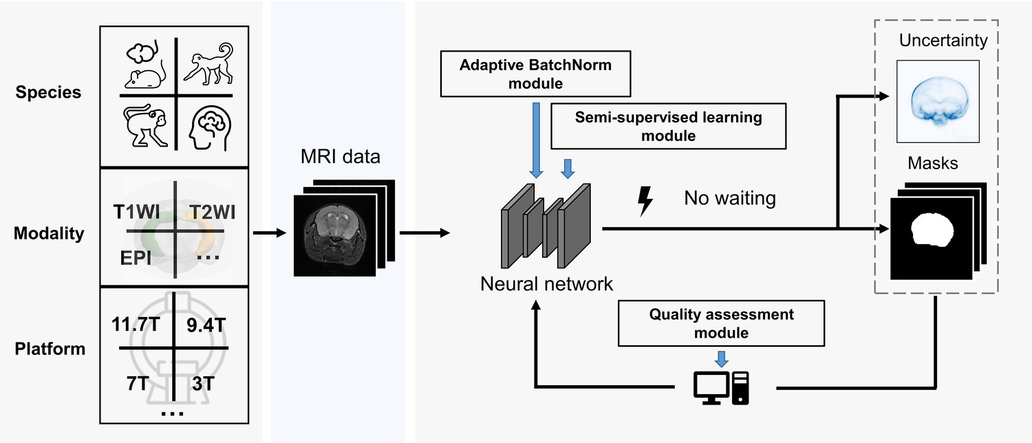
BEN renovates the brain extraction workflow to adapt to multiple species, modalities and platforms.
The BEN has the following advantages: (1) Transferability and flexibility: BEN can adapt to different species, modalities and platforms through its adaptive batch normalization module and semi-supervised learning module. (2) Automatic quality assessment: Unlike traditional toolboxes, which rely on manual inspection to assess the brain extraction quality, BEN incorporates a quality assessment module to automatically evaluate its brain extraction performance. (3) Speed: As a DL-based method, BEN can process an MRI volume faster (<1 s) than traditional toolboxes (several minutes or longer).
Figure 2

The architecture of our proposed BEN demonstrates its generalizability.
(A) The domain transfer workflow. BEN is initially trained on the Mouse-T2-11.7T dataset (representing the source domain) and then transferred to many target domains that differ from the source domain in either the species, MRI modality, magnetic field strength, or some combination thereof. Efficient domain transfer is achieved via an adaptive batch normalization (AdaBN) strategy and a Monte Carlo quality assessment (MCQA) module. (B) The backbone of BEN is the nonlocal U-Net (NL-U-Net) used for brain extraction. Similar to the classic U-Net architecture, NL-U-Net also contains a symmetrical encoding and decoding path, with an additional nonlocal attention module to tell the network where to look, thus maximizing the capabilities of the model. (C) Illustration of the AdaBN strategy. The batch normalization (BN) layers in the network are first trained on the source domain. When transferring to a target domain, the statistical parameters in the BN layers are updated in accordance with the new data distribution in the target domain. (D) Illustration of the MCQA process. We use Monte Carlo dropout sampling during the inference phase to obtain multiple predictions in a stochastic fashion. The Monte Carlo predictions are then used to generate aleatoric and epistemic uncertainties that represent the confidence of the segmentations predicted by the network, and we screen out the optimal segmentations with minimal uncertainty in each batch and use them as pseudo-labels for semi-supervised learning.
Figure 3 with 4 supplements
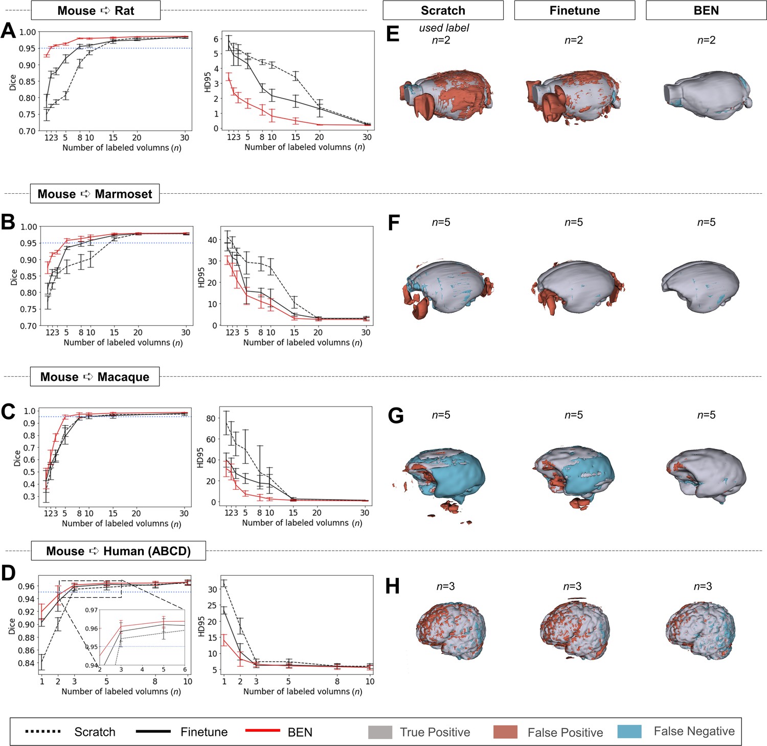
Performance comparison of BEN with two benchmark settings on the task of cross-species domain transfer.
(A - D) Curve plots representing domain transfer tasks across species, showing the variation in the segmentation performance in terms of the Dice score and 95% Hausdorff distance (HD95) (y axis) as a function of the number of labeled volumes (x axis) for training from scratch (black dotted lines), fine-tuning (black solid lines) and BEN (red lines). From top to bottom: (A) mouse to rat, (B) mouse to marmoset, (C) mouse to macaque, and (D) mouse to human (ABCD) with an increasing amount of labeled training data (n=1, 2, 3, …, as indicated on the x axis in each panel). Both the Dice scores and the HD95 values of all three methods reach saturation when the number of labels is sufficient (n>20 labels); however, BEN outperforms the other methods, especially when limited labels are available (n≤5 labels). Error bars represent the mean with a 95% confidence interval (CI) for all curves. The blue dotted line corresponds to y(Dice)=0.95, which can be considered to represent qualified performance for brain extraction. (E - H) 3D renderings of representative segmentation results (the number (n) of labels used for each method is indicated in each panel). Images with fewer colored regions represent better segmentation results. (gray: true positive; brown: false positive; blue: false negative). Sample size for these datasets: Mouse-T2WI-11.7T (N=243), Rat-T2WI-11.7T (N=132), Marmoset-T2WI-9.4T (N=62), Macaque-T1WI (N=76) and Human-ABCD (N=963).
Figure 3—figure supplement 1
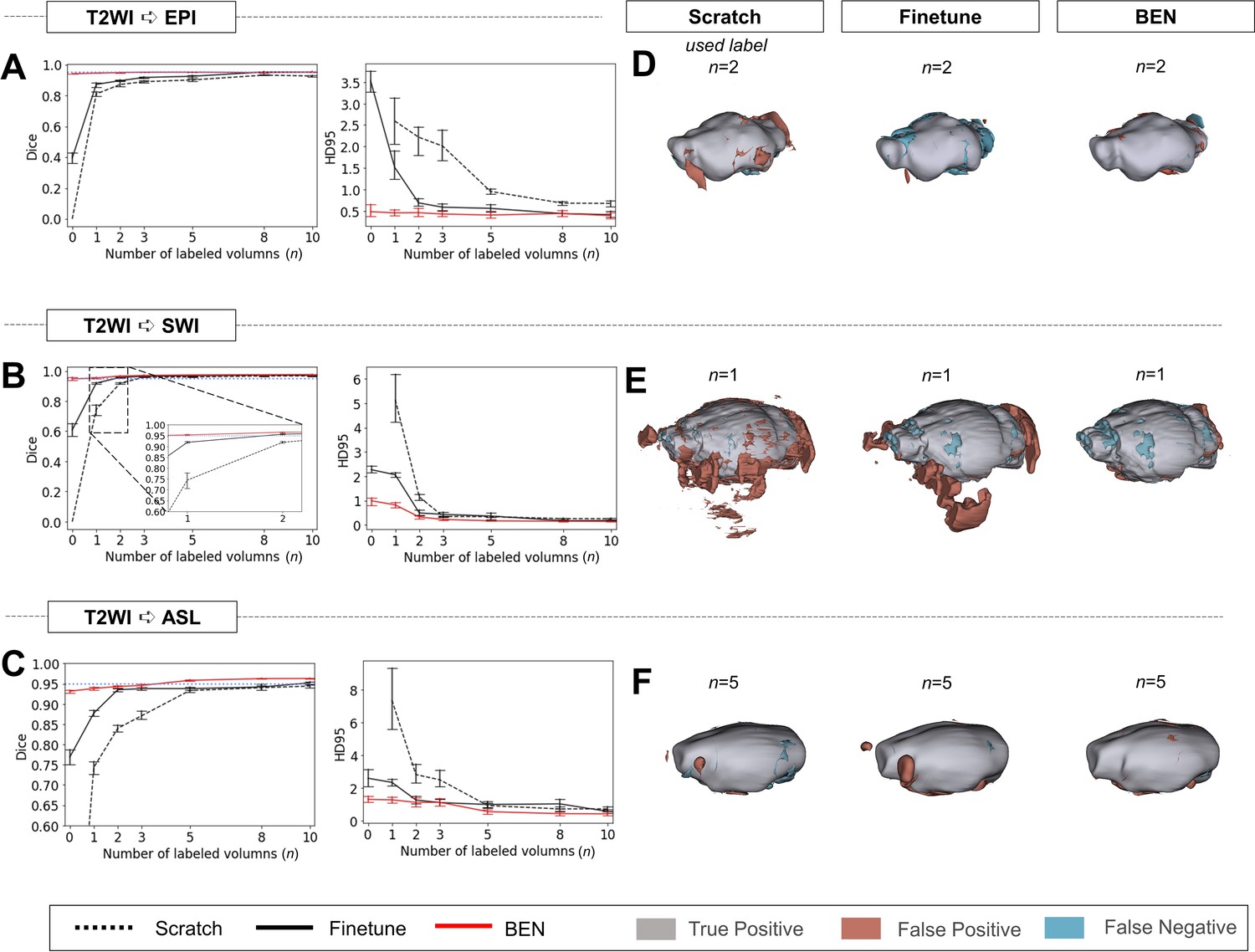
Performance comparison of BEN with two benchmark settings on the task of cross-modality domain transfer.
(A - C) The curve plots representing domain transfer tasks across modality, showing the variation in the segmentation performance in terms of the Dice score and 95% Hausdorff distance (HD95) (y axis) as a function of the number of labeled volumes (x axis) for training from scratch (black dotted lines), fine-tuning (black solid lines) and BEN (red lines). From top to bottom: (A) T2WI to EPI, (B) T2WI to SWI and (C) T2WI to ASL with an increasing amount of labeled training data (n=1, 2, 3, 5, 8, 10, as indicated on the x axis in each panel). BEN consistently surpasses other methods with less labeled data required. Note that, BEN achieves acceptable performance via zero-shot inference (n=0), where no label is used in the target domain. In this case, fine-tuning directly infer on target datasets and training from scratch failed to perform. Error bars represent the mean with a 95% confidence interval (CI) for all curves. The blue dotted line corresponds to y(Dice)=0.95, which can be considered to represent qualified performance for brain extraction. (D - F) 3D renderings of representative segmentation results (the number (n) of labels used for each method is indicated in each panel). Images with fewer colored regions represent better segmentation results. (gray: true positive; brown: false positive; blue: false negative). Sample size for these datasets: Mouse-T2WI-11.7T (N=243), Mouse-EPI-11.7T (N=54), Mouse-SWI-11.7T (N=50) and Mouse-ASL-11.7T (N=58).
Figure 3—figure supplement 2
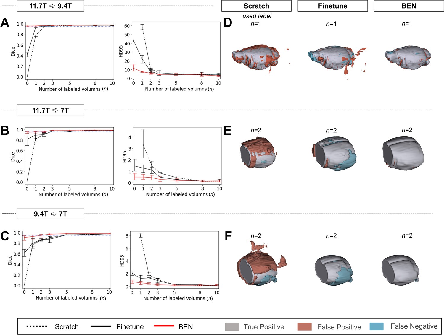
Performance comparison of BEN with two benchmark settings on the task of cross-platform domain transfer.
(A - C) Curve plots representing domain transfer tasks across platforms with different magnetic field strengths, showing the variation in the segmentation performance in terms of the Dice score and 95% Hausdorff distance (HD95) (y axis) as a function of the number of labeled volumes (x axis) for training from scratch (black dotted lines), fine-tuning (black solid lines) and BEN (red lines). From top to bottom: (A) 11.7T to 9.4T, (B) 11.7T to 7T and (C) 9.4T to 7T with an increasing amount of labeled training data (n=1, 2, 3,..., as indicated on the x axis in each panel). BEN reaches saturation point much earlier in all three tasks than other methods, indicating that fewer labels are required for BEN than for other methods. Error bars represent the mean with a 95% confidence interval (CI) for all curves. The blue dotted line corresponds to y(Dice)=0.95, which can be considered to represent qualified performance for brain extraction. (D - F) 3D renderings of representative segmentation results (the number (n) of labels used for each method is indicated in each panel). Note that due to MRI acquisition, the anterior and posterior of brains in the 7T dataset are not included. Images with fewer colored regions represent better segmentation results. (gray: true positive; brown: false positive; blue: false negative). Sample size for these datasets: Mouse-T2WI-11.7T (N=243), Mouse-T2WI-9.4T (N=14), Mouse-T2WI-7T (N=14).
Figure 3—figure supplement 3
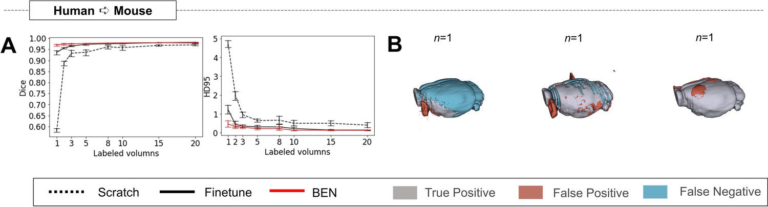
BEN’s transferability is not dependent on specific source dataset.
In our previous experiments, the mouse-T2WI-11.7T dataset was used as the source domain and transferred the model to other species, including humans. Here, we reselect the human as the source domain and transfer the model to the mouse dataset. (A) Human to Mouse with an increasing amount of labeled training data (n=1, 2, 3,..., as indicated on the x axis in each panel). Curve plots representing domain transfer tasks across species, showing the variation in the segmentation performance in terms of HD95 (y axis) as a function of the number of labeled volumes (x axis) for training from scratch (black dotted lines), fine-tuning (black solid lines), and BEN (red lines). (B) 3D renderings of representative segmentation results (the number (n) of labels used for each method is indicated in each panel). Images with fewer colored regions represent better segmentation results. (gray: true positive; brown: false positive; blue: false negative). Sample size for these datasets: Mouse-T2WI-11.7T (N=243) and Human-ABCD (N=3250).
Figure 3—figure supplement 4
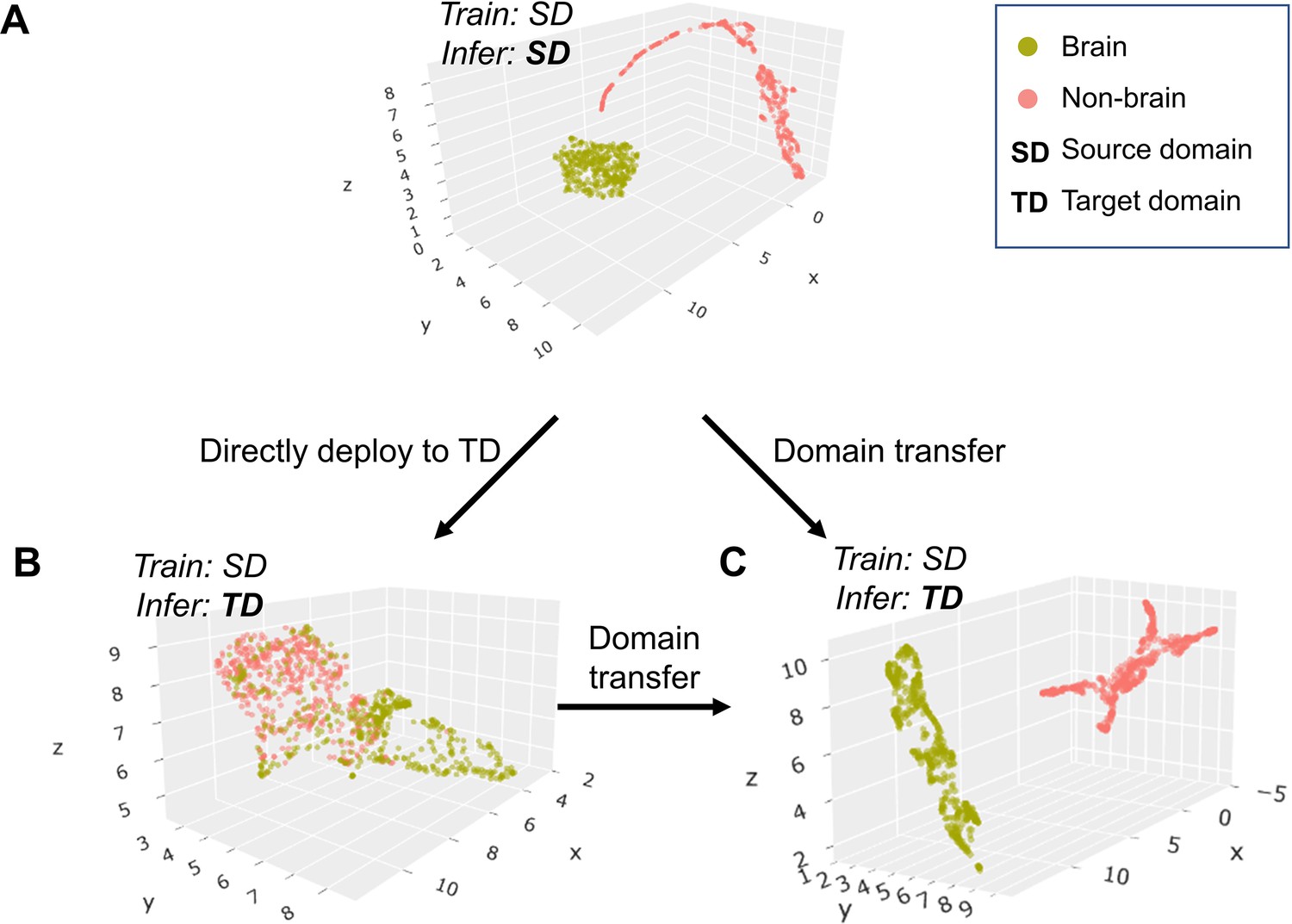
UMAP visualizes BEN’s transfer learning.
(A - C) Scatter plot of neural network feature map clusters. An unsupervised clustering algorithm (UMAP) was used to visualize the semantic features. Different colors in the scatter plot indicate different clusters (green: brain, red: non-brain). Visualization of feature maps via UMAP during the following three intermediate processes: (A) semantic features of brain and non-brain are separate in the source domain; (B) these features are intermingled in the target domain without transfer learning; (C) features are separated again in the target domain after BEN’s domain transferring strategy.
Figure 4 with 4 supplements
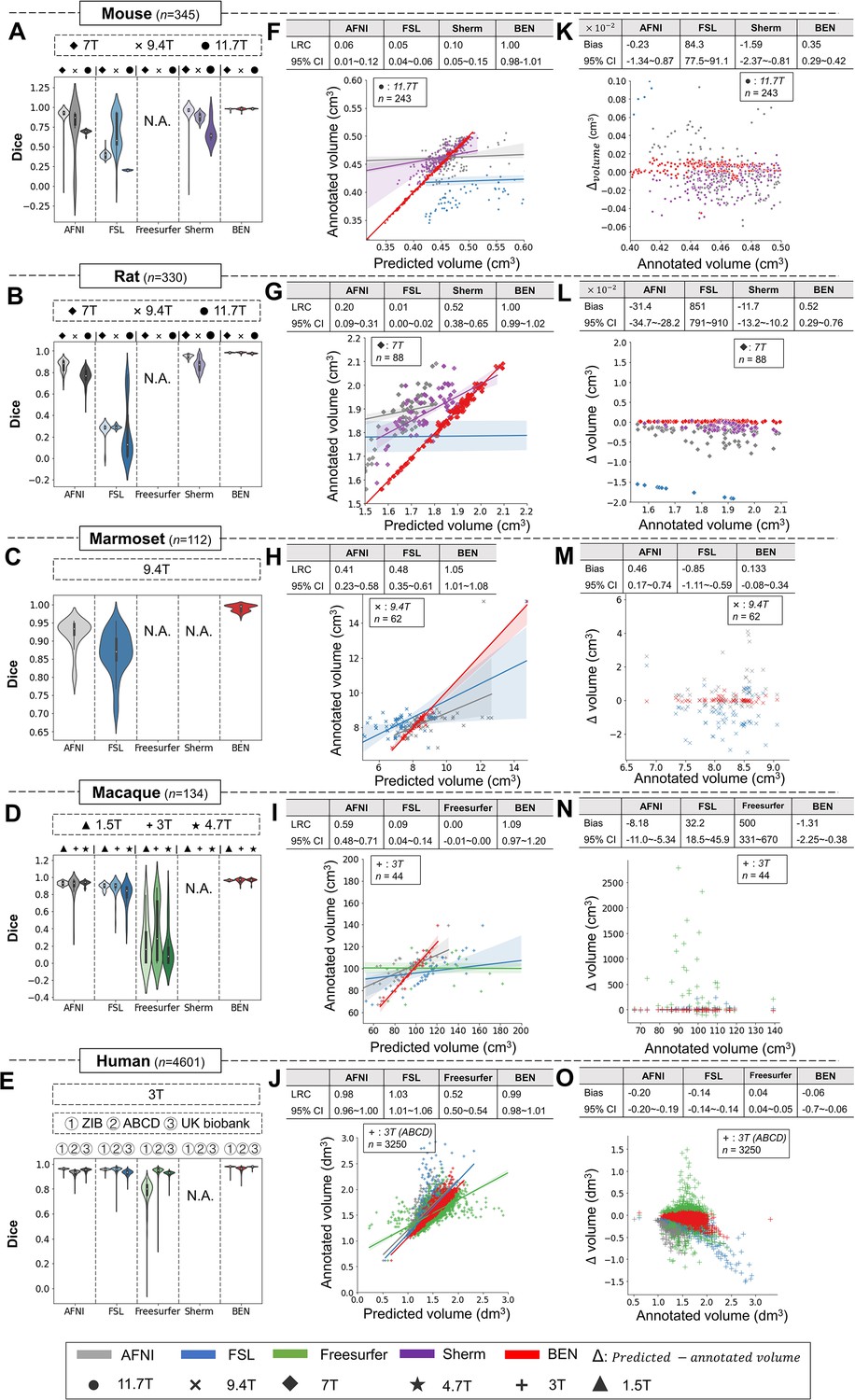
BEN outperforms traditional SOTA methods and advantageously adapts to datasets from various domains across multiple species, modalities, and field strengths.
(A - E) Violin plots and inner box plots showing the Dice scores of each method for (A) mouse (n=345), (B) rat (n=330), (C) marmoset (n=112), (D) macaque (n=134), and (E) human (n=4601) MRI scans acquired with different magnetic field strengths. The field strength is illustrated with different markers above each panel, and the results for each method are shown in similar hues. The median values of the data are represented by the white hollow dots in the violin plots, the first and third quartiles are represented by the black boxes, and the interquartile range beyond 1.5 times the first and the third quartiles is represented by the black lines. ‘N.A.’ indicates a failure of the method on the corresponding dataset. (F - J) Comparisons of the volumetric segmentations obtained with each method relative to the ground truth for five species. For better visualization, we select magnetic field strengths of 11.7T for mouse scans (F), 7T for rat scans (G), 9.4T for marmoset scans (H), and 3T for both macaque (I) and human (J) scans. Plots for other field strengths can be found in Figure 4—figure supplement 2. The linear regression coefficients (LRCs) and 95% CIs are displayed above each graph. Each dot in a graph represents one sample in the dataset. The error bands in the plots represent the 95% CIs. (K - O) Bland–Altman analysis showing high consistency between the BEN results and expert annotations. The biases between two observers and the 95% CIs for the differences are shown in the tables above each plot. Δvolume = predicted volume minus annotated volume. Each method is shown using the same hue in all plots (gray: AFNI; blue: FSL; green: FreeSurfer; purple: Sherm; red: BEN). Different field strengths are shown with different markers (●: 11.7T; ×: 9.4T; ◆: 7T; ★: 4.7T; +: 3T; ▲: 1.5T). The Dice scores compute the overlap between the segmentation results and manual annotations.
Figure 4—figure supplement 1
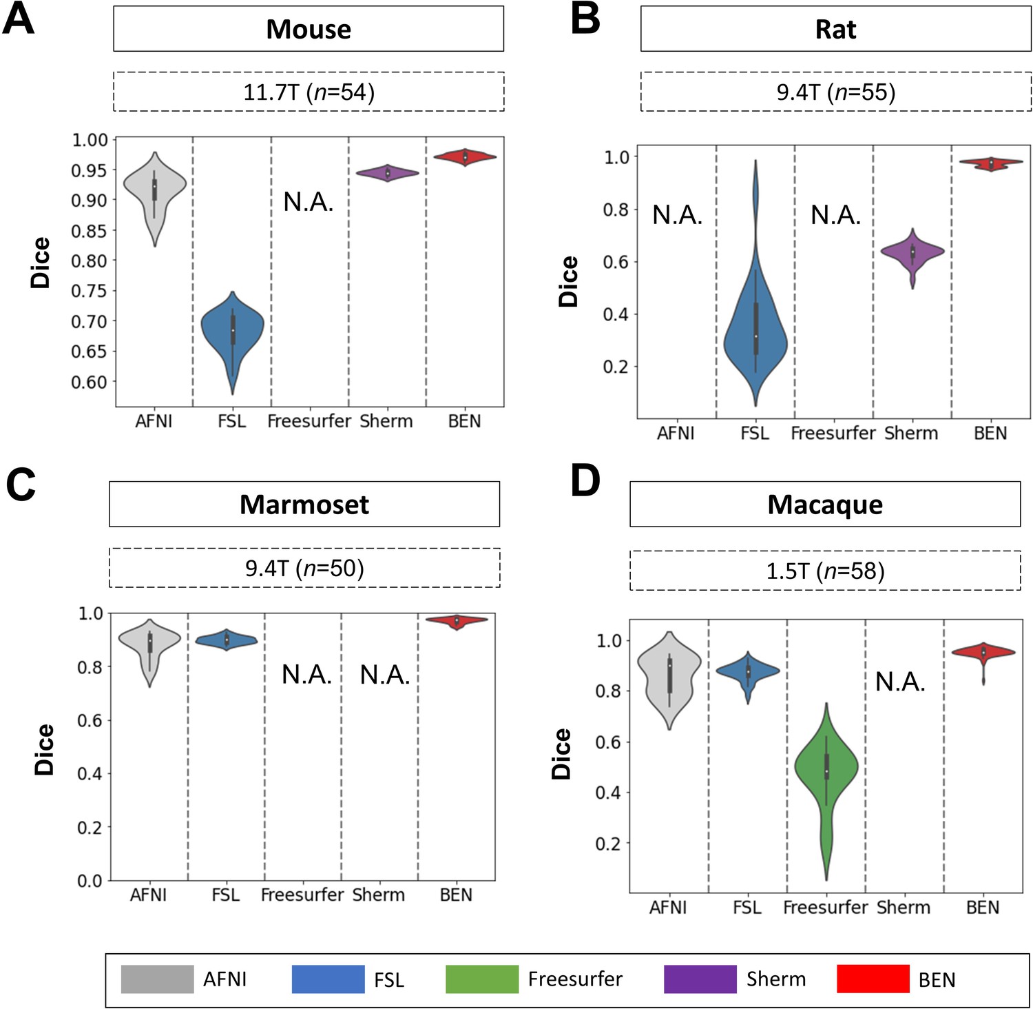
BEN outperforms traditional SOTA methods in functional MRI scans acquired from multiple species on different magnetic field strengths.
(A - D) Violin plots and inner box plots showing the Dice scores of each method for (A) mouse (n=54), (B) rat (n=55), (C) marmoset (n=50), and (d) macaque (n=58) MRI images acquired. The field strength is illustrated with different markers above each panel, and the results for each method are shown in similar hues. The median values of the data are represented by the white hollow dots in the violin plots, the first and third quartiles are represented by the black boxes, and the interquartile range beyond 1.5 times the first and the third quartiles is represented by the black lines. ‘N.A.’ indicates failure of the method on the corresponding dataset. (gray: AFNI; blue: FSL; green: Freesurfer; purple: Sherm; red: BEN).
Figure 4—figure supplement 2
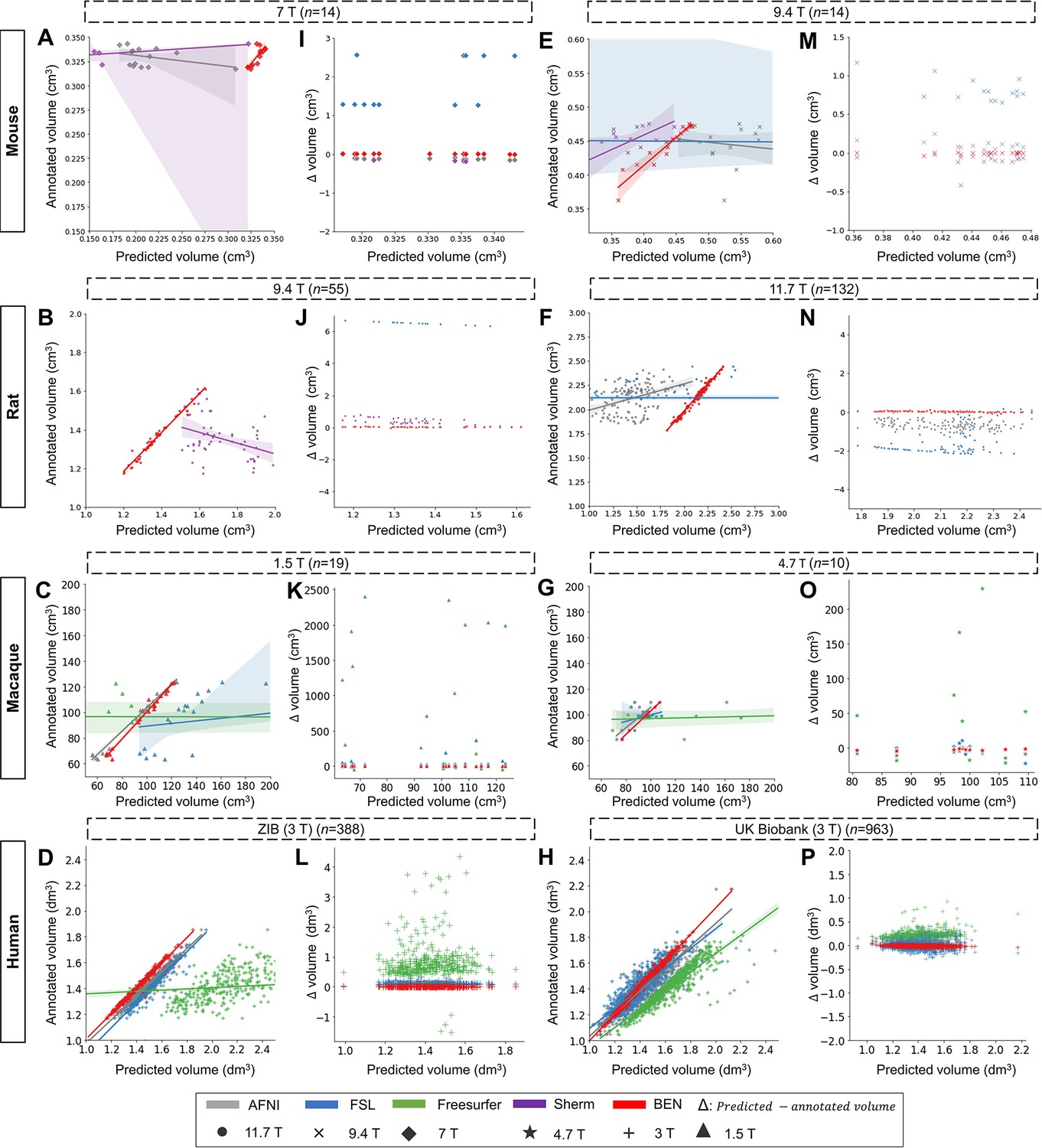
Linear regression coefficients and Bland–Altman analysis demonstration of the rest datasets.
(A–D, E–H) The segmentation accuracy is assessed using the linear regression coefficients (LRCs) (n of volumes used are shown above the figure panels). Compared with other methods, BEN achieves better performance. The magnetic field strengths are also shown in different markers according to the legend. Each dot in a graph represents one sample in the dataset. The error bands represent 95% CI in plots. (I - L, M - P) Bland–Altman analysis showing high consistency between the BEN results and expert annotations. The biases between two observers and the 95% CIs for the differences are shown in the tables above each plot. Each method is shown using the same hue in all plots (gray: AFNI; blue: FSL; green: FreeSurfer; purple: Sherm; red: BEN). Different field strengths are shown with different markers (●: 11.7T; ×: 9.4T; ◆: 7T; ★: 4.7T; +: 3T; ▲: 1.5T).
Figure 4—figure supplement 3
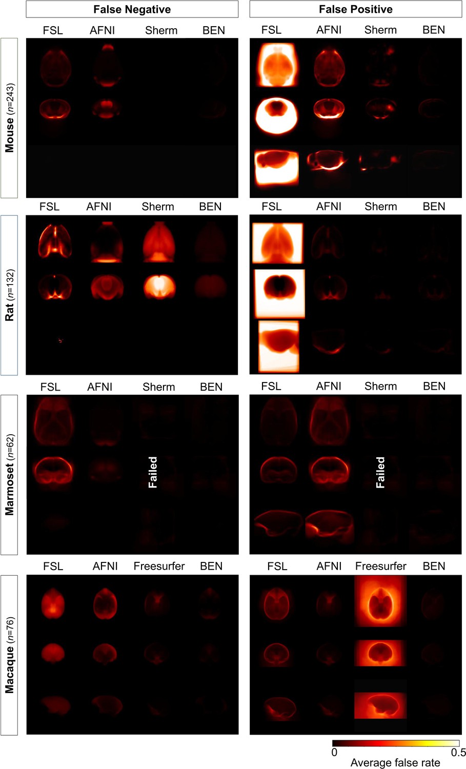
Error maps of BEN and SOTA methods.
Heatmap projections of average false negative (FN) and false positive (FP) for each species (mouse, rat, marmoset, and macaque). From the first row to the third row: axial, coronal, and sagittal view. Compared with other methods, BEN shows much less FN and FP errors. The upper extreme represents a high systematic number of FNs and FPs. (mouse: n=243 in Mouse-T2WI-11.7T dataset; rat: n=132 in Rat-T2WI-11.7T dataset; marmoset: n=62 in Marmoset-T2WI-9.4T dataset; macaque: n=76 in Macaque-T1WI dataset).
Figure 4—figure supplement 4
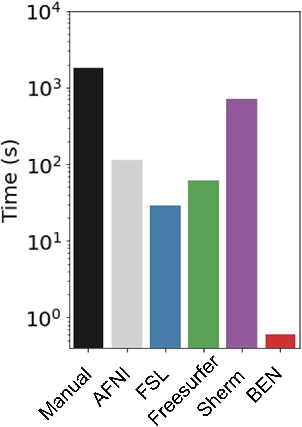
Execution time comparison of BEN with other methods.
Compared with other conventional methods, BEN has unequaled faster processing speed. The plot is in log scale and represents average processing time to segment one 3D volume.
Figure 5 with 1 supplement

BEN improves the accuracy of atlas registration by producing high-quality brain extraction results.
(A) The Dorr space, (E) the SIGMA space and (I) the MNI space, corresponding to the mouse, rat and human atlases, respectively. (B, F, J) Integration of BEN into the registration workflow: (i) Three representative samples from a mouse (n=157), a rat (n=88), and human (n=144) in the native space. (ii) The BEN-segmented brain MRI volumes in the native space as registered into the Dorr/SIGMA/MNI space using the Advanced Normalization Tools (ANTs) toolbox, for comparison with the registration of AFNI-segmented/original MRI volumes with respect to the corresponding atlas. (iii) The warped volumes in the Dorr/SIGMA/MNI spaces. (iv) Error maps showing the fixed atlas in green and the moving warped volumes in magenta. The common areas where the two volumes are similar in intensity are shown in gray. (v) The brain structures in the warped volumes shown in the atlas spaces. In our experiment, BEN significantly improves the alignment between the propagated annotations and the atlas, as confirmed by the improved Dice scores in the (C, G, K) thalamic and (D, H, L) hippocampal regions (box plots: purple for BEN, green for w/o BEN; volumes: n=157 for the mouse, n=88 for the rat, n=144 for the human; statistics: paired t-test, n.s.: no significance, *p<0.05, **p<0.01, ***p<0.001).
Figure 5—figure supplement 1
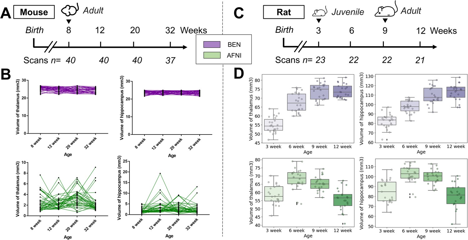
Atlas registration with BEN benefits brain volumetric quantification in longitudinal studies.
In our two examples, (A) adult mice (n=40) were imaged at weeks 8, 12, 20, and 32. (B) With BEN (purple boxplots), the volume statistics of the thalamus and hippocampus remain almost constant, which is plausible, as these two brain regions do not further enlarge in adulthood. In comparison, (D) the volume changes of the thalamus and hippocampus in (C) juvenile rats (n=23, imaged at weeks 3, 6, 9, and 12) suggest continuous growth with time, particularly between weeks 3 and 9. In contrast, with AFNI, due to poor atlas registration and consequently inaccurate volume statistics (green box plots), these crucial brain growth trends during development may be missed.
Figure 6 with 3 supplements
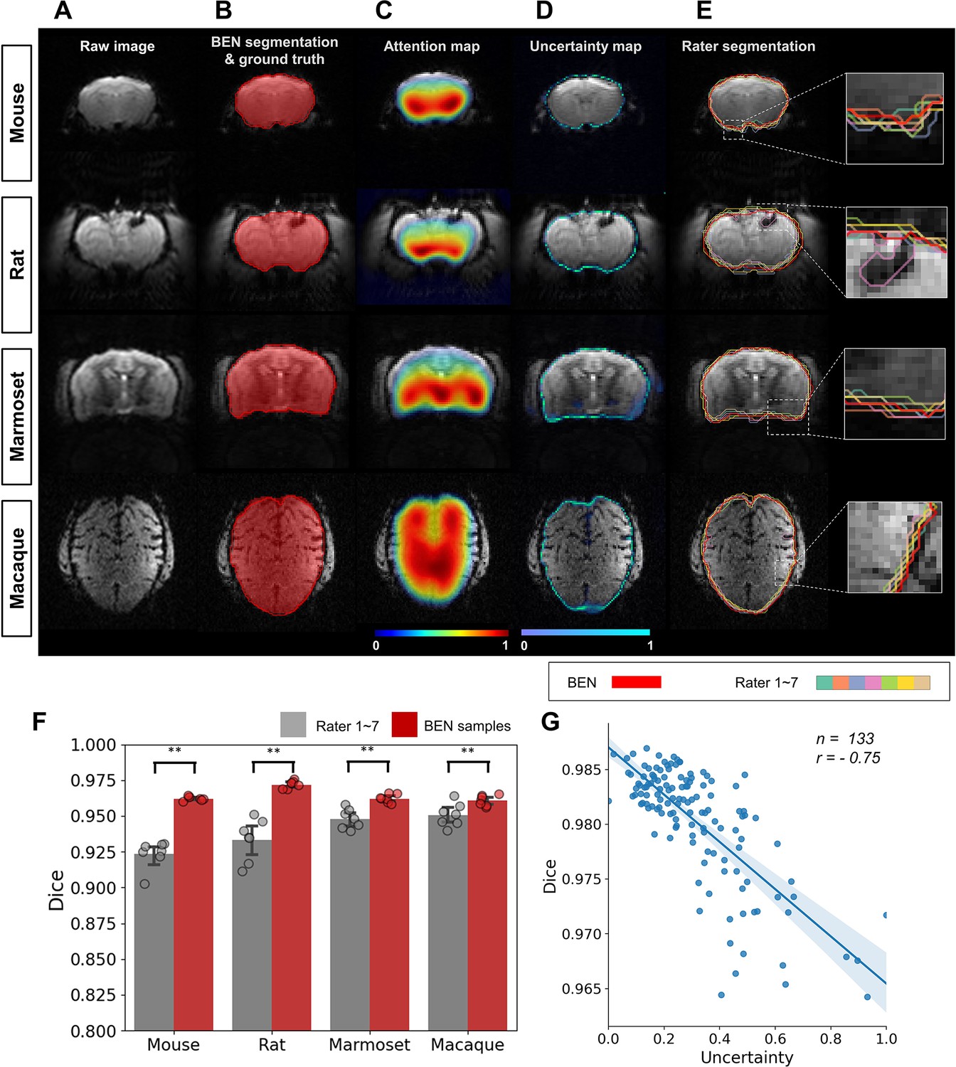
BEN provides a measure of uncertainty that potentially reflects rater disagreement.
(A) Representative EPI images from four species (in each column from left to right, mouse, rat, marmoset, and macaque). (B) BEN segmentations (red semi-transparent areas) overlaid with expert consensus annotations (red opaque lines), where the latter are considered the ground truth. (C) Attention maps showing the key semantic features in images as captured by BEN. (D) Uncertainty maps showing the regions where BEN has less confidence. The uncertainty values are normalized (0–1) for better visualization. (E) Annotations by junior raters (n=7) shown as opaque lines of different colors. (F) Bar plots showing the Dice score comparisons between the ground truth and the BEN segmentation results (red) as well as the ground truth and the junior raters’ annotations (gray) for all species (gray: raters, n=7, red: Monte Carlo samples from BEN, n=7; statistics: Mann–Whitney test, **p<0.01). Each dot represents one rater or one sample. Values are represented as the mean and 95% CI. (G) Correlation of the linear regression plot between the Dice score and the normalized uncertainty. The error band represents the 95% CI. Each dot represents one volume (species: mouse; modality: T2WI; field strength: 11.7T; n=133; r=−0.75).
Figure 6—figure supplement 1
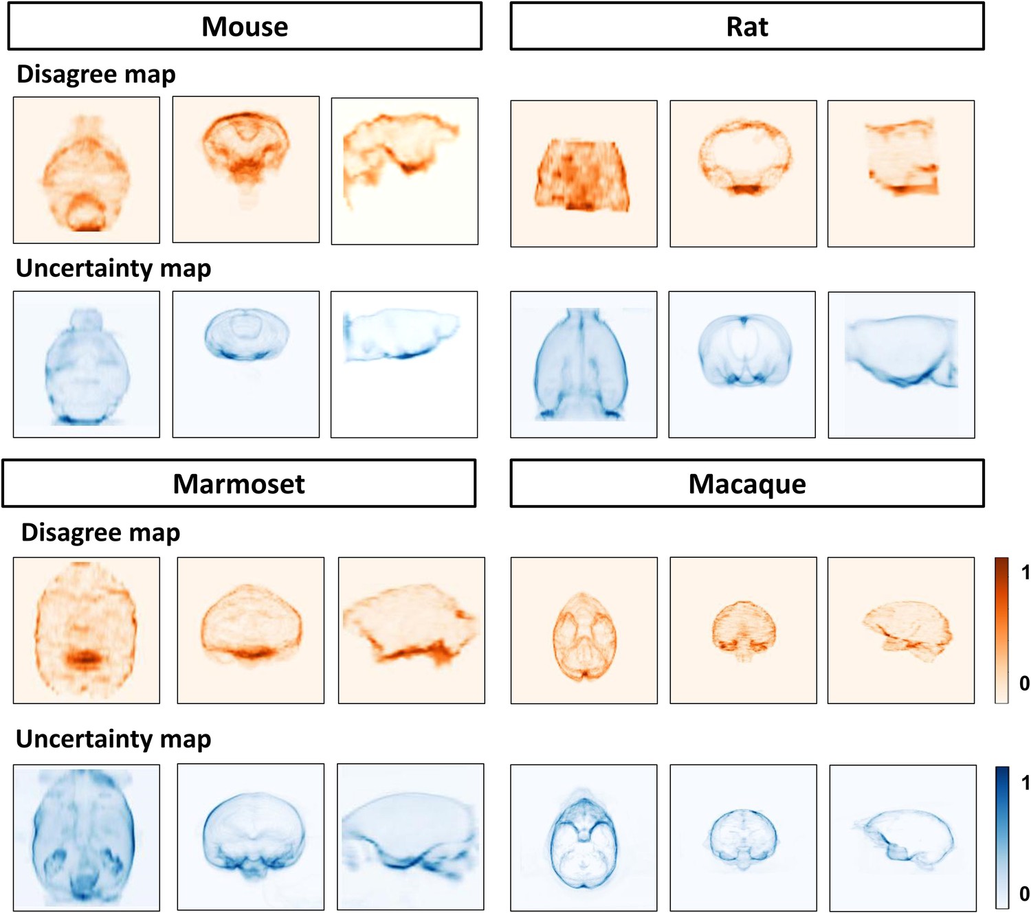
BEN’s uncertainty is consistent with interrater' disagreement.
Heat map projections of raters’ disagreement (orange hues) and BEN uncertainty (blue hues) across four species using the ground truth as the reference. From left to right: Sagittal, coronal and axial view. These disagree maps and uncertainty maps share similar feature distribution patterns.
Figure 6—figure supplement 2
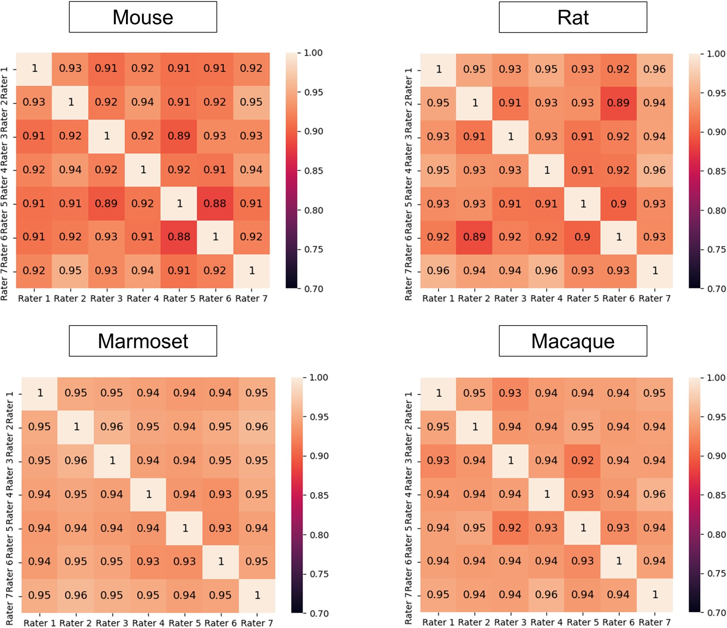
Interrater disagreement.
Heatmaps representing the segmentation Dice scores of each junior rater as calculated using the labels from one of the others as the ground truth on the rat images and the macaque images.
Figure 6—figure supplement 3
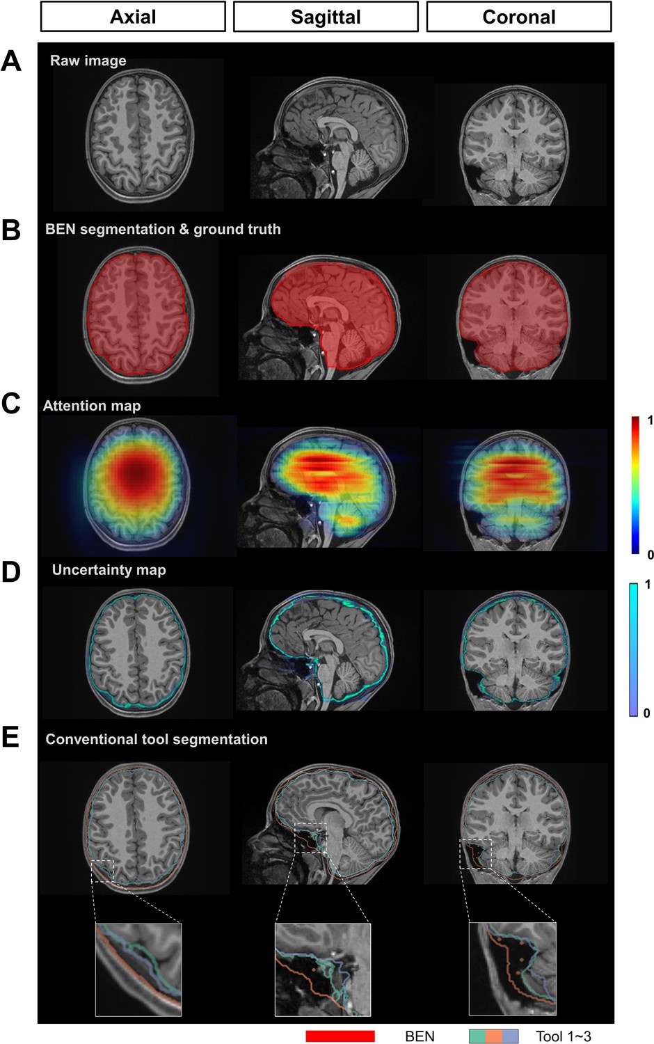
BEN provides a measure of uncertainty that potentially reflects the disagreement of conventional toolboxes in human data.
(A) Representative structural MR images of the human in the ABCD dataset (n=3250). (B) BEN’s segmentation (red semi-transparent areas) overlaid with annotation of experts’ consensus, which is considered as ground truth (red opaque lines). (C) Attention map shows the key semantic features in images where BEN captures. (D) Uncertainty map shows the regions where BEN has less confidence. The uncertainty values are normalized (0~1) for better visualization. (E) Segmentations obtained by toolboxes (n=3) are shown in different color opaque lines.
Tables
Appendix 1—table 1
MRI scan information of the fifteen animal datasets and three human datasets.
FDU: Fudan University. UCAS: University of Chinese Academy of Sciences; UNC: University of North Carolina at Chapel Hill; ABCD: Adolescent Brain Cognitive Developmental study; ZIB: Zhangjiang International Brain BioBank at Fudan University.
| Species | Modality | Magnetic Field(T) | Scans | Slices | In-plane Resolution(mm) | Thickness(mm) | Manufacturer | Institution |
|---|---|---|---|---|---|---|---|---|
| Mouse | T2WI | 11.7 | 243 | 9,030 | 0.10*0.10 | 0.4 | Bruker | FDU |
| 9.4 | 14 | 448 | 0.06*0.06 | 0.4 | Bruker | UCAS | ||
| 7 | 14 | 126 | 0.08*0.08 | 0.8 | Bruker | UCAS | ||
| EPI | 11.7 | 54 | 2,198 | 0.2*0.2 | 0.4 | Bruker | FDU | |
| 9.4 | 20 | 360 | 0.15*0.15 | 0.5 | Bruker | UCAS | ||
| SWI | 11.7 | 50 | 1,500 | 0.06*0.06 | 0.5 | Bruker | FDU | |
| ASL | 11.7 | 58 | 696 | 0.167*0.167 | 1 | Bruker | FDU | |
| Rat | T2WI | 11.7 | 132 | 5,544 | 0.14*0.14 | 0.6 | Bruker | FDU |
| 9.4 | 55 | 660 | 0.1*0.1 | 1 | Bruker | UNC † | ||
| 7 | 88 | 4,400 | 0.09*0.09 | 0.4 | Bruker | UCAS | ||
| EPI | 9.4 | 55 | 660 | 0.32*0.32 | 1 | Bruker | UNC † | |
| Sum of rodent | 783 | 25,622 | ||||||
| Marmoset | T2WI | 9.4 | 62 | 2,480 | 0.2*0.2 | 1 | Bruker | UCAS |
| EPI | 9.4 | 50 | 1,580 | 0.5*0.5 | 1 | Bruker | UCAS | |
| Macaque * | T1WI | 4.7 3 1.5 | 76 | 20,063 | 0.3*0.3~0.6*0.6 | 0.3~0.75 | Siemens, Bruker, Philips | Multicenter |
| EPI | 1.5 | 58 | 2,557 | 0.7*0.7~2.0*2.0 | 1.0~3.0 | Siemens, Bruker, Philips | Multicenter | |
| Sum of nonhuman primate | 246 | 26,680 | ||||||
| Human (ABCD) | T1WI | 3 | 3,250 | 552,500 | 1.0*1.0 | 1 | GE Siemens Philips | Multicenter |
| Human (UK Biobank) | T1WI | 3 | 963 | 196,793 | 1.0*1.0 | 1 | Siemens | Multicenter |
| Human (ZIB) | T1WI | 3 | 388 | 124,160 | 0.8*0.8 | 0.8 | Siemens | FDU |
| Sum of human | 4,601 | 873,453 | ||||||
| In total | 5,630 | 925,755 |
-
*
-
†
Appendix 1—table 2
Performance comparison of BEN with SOTA methods on the source domain (Mouse-T2WI-11.7T).
Dice: Dice score; SEN: sensitivity; SPE: specificity; ASD: Average Surface Distance; HD95: the 95-th percentile of Hausdorff distance.
| Method | Dice | SEN | SPE | ASD | HD95 |
|---|---|---|---|---|---|
| Sherm | 0.9605 | 0.9391 | 0.9982 | 0.6748 | 0.4040 |
| AFNI | 0.9093 | 0.9162 | 0.9894 | 1.9346 | 0.9674 |
| FSL | 0.3948 | 1.0000 | 0.6704 | 20.4724 | 5.5975 |
| BEN | 0.9859 | 0.9889 | 0.9982 | 0.3260 | 0.1436 |
Appendix 1—table 3
Performance comparison of BEN with SOTA methods on two public datasets.
Dice: Dice score; Jaccard: Jaccard Similarity; SEN: sensitivity; HD: Hausdorff distance.
| CARMI dataset * (Rodent) | ||||
|---|---|---|---|---|
| T2WI | ||||
| Methods | Dice | Jaccard | SEN | HD (voxels) |
| RATS (Oguz et al., 2014) | 0.91 | 0.83 | 0.85 | 8.76 |
| PCNN (Chou et al., 2011) | 0.89 | 0.80 | 0.90 | 7.00 |
| SHERM (Liu et al., 2020) | 0.88 | 0.79 | 0.86 | 6.72 |
| U-Net (Hsu et al., 2020) | 0.97 | 0.94 | 0.96 | 4.27 |
| BEN | 0.98 | 0.95 | 0.98 | 2.72 |
| EPI | ||||
| Methods | Dice | Jaccard | SEN | HD (voxels) |
| RATS (Oguz et al., 2014) | 0.86 | 0.75 | 0.75 | 7.68 |
| PCNN (Chou et al., 2011) | 0.85 | 0.74 | 0.93 | 8.25 |
| SHERM (Liu et al., 2020) | 0.80 | 0.67 | 0.78 | 7.14 |
| U-Net (Hsu et al., 2020) | 0.96 | 0.93 | 0.96 | 4.60 |
| BEN | 0.97 | 0.94 | 0.98 | 4.20 |
| PRIME-DE † (Macaque) | ||||
| T1WI | ||||
| Methods | Dice | Jaccard | SEN | HD (voxels) |
| FSL | 0.81 | 0.71 | 0.96 | 32.38 |
| FreeSurfer | 0.56 | 0.39 | 0.99 | 42.18 |
| AFNI | 0.86 | 0.79 | 0.82 | 25.46 |
| U-Net (Wang et al., 2021) | 0.98 | - | - | - |
| BEN | 0.98 | 0.94 | 0.98 | 13.21 |
-
*
-
†
Appendix 1—table 4
Ablation study of each module of BEN in the source domain.
(a) training with all labeled data using U-Net. The backbone of BEN is non-local U-Net (NL-U-Net). (b) training with 5% labeled data. (c) training with 5% labeled data using BEN’s semi-supervised learning module (SSL). The remaining 95% of the unlabeled data is also used for the training. Since this ablation study is performed on the source domain, the adaptive batch normalization (AdaBN) module is not used. Dice: Dice score; SEN: sensitivity; SPE: specificity; HD95: the 95-th percentile of Hausdorff distance.
| Method | Scans used | Metrics | ||||
|---|---|---|---|---|---|---|
| Labeled | Unlabeled | Dice | SEN | SPE | HD95 | |
| aU-Net | 243 | 0 | 0.9773 | 0.9696 | 0.9984 | 0.2132 |
| aBackbone | 243 | 0 | 0.9844 | 0.9830 | 0.9984 | 0.0958 |
| bU-Net | 12 | 0 | 0.9588 | 0.9546 | 0.9945 | 1.1388 |
| bBackbone | 12 | 0 | 0.9614 | 0.9679 | 0.9970 | 0.7468 |
| cBackbone +SSL | 12 | 231 | 0.9728 | 0.9875 | 0.9952 | 0.2937 |
Appendix 1—table 5
Ablation study of each module of BEN in the target domain.
(a) training from scratch with all labeled data. The backbone of BEN is non-local U-Net (NL-U-Net). (b) training from scratch with 5% labeled data. (c) fine-tuning (using pretrained weights) with 5% labeled data. (d) fine-tuning with 5% labeled data using BEN’s SSL and AdaBN modules. The remaining 95% of the unlabeled data is also used for the training stage. Dice: Dice score; SEN: sensitivity; SPE: specificity; HD95: the 95-th percentile of Hausdorff distance.
| Method | Pretrained | Scans used | Metrics | ||||
|---|---|---|---|---|---|---|---|
| Labeled | Unlabeled | Dice | SEN | SPE | HD95 | ||
| aBackbone (from scratch) | 132 | 0 | 0.9827 | 0.9841 | 0.9987 | 0.1881 | |
| bBackbone (from scratch) | 7 | 0 | 0.8990 | 0.8654 | 0.9960 | 4.6241 | |
| cBackbone | ✓ | 7 | 0 | 0.9483 | 0.9063 | 0.9997 | 0.6563 |
| cBackbone +AdaBN | ✓ | 7 | 0 | 0.9728 | 0.9875 | 0.9952 | 0.2937 |
| dBackbone +SSL | ✓ | 7 | 125 | 0.9614 | 0.9679 | 0.9970 | 0.7468 |
| dBackbone +AdaBN + SSL | ✓ | 7 | 125 | 0.9779 | 0.9763 | 0.9986 | 0.2912 |
Appendix 1—table 6
BEN provides interfaces for the following conventional neuroimaging software.
Appendix 1—table 7
Protocols and parameters used for conventional neuroimaging toolboxes.
| Method | Command | Parameter | Description | Range | Chosen value | |
|---|---|---|---|---|---|---|
| AFNI | 3dSkullStrip | -marmoset | Brain of a marmoset | on/off | on for marmoset | |
| -rat | Brain of a rat | on/off | on for rodent | |||
| -monkey | Brain of a monkey | on/off | on for macaque | |||
| FreeSurfer | mri_watershed | -T1 | Specify T1 input volume | on/off | on | |
| -r | Specify the radius of the brain (in voxel unit) | positive number | 60 | |||
| -less | Shrink the surface | on/off | off | |||
| -more | Expand the surface | on/off | off | |||
| FSL | bet2 | -f | Fractional intensity threshold | 0.1~0.9 | 0.5 | |
| -m | Generate binary brain mask | on/off | on | |||
| -n | Don't generate the default brain image output | on/off | on | |||
| Sherm | sherm | -animal | Species of the task | 'rat' or 'mouse' | according to the task | |
| -isotropic | Characteristics of voxels | 0/1 | 0 | |||
Author response table 1
Comparison of brain extraction performance of different methods on different datasets.
SkullStrip: semi-automatic registration-based method. (ASD: average surface distance. HD95: 95% Hausdorff distance).
| Species | Field | Modality | Method | Dice | Sensitivity | Specificity | ASD | HD95 |
|---|---|---|---|---|---|---|---|---|
| Mouse | 11.7T | T2WI | BEN | 0.9859 | 0.9889 | 0.9982 | 0.3260 | 0.1436 |
| Sherm | 0.9605 | 0.9391 | 0.9982 | 0.6748 | 0.4040 | |||
| AFNI | 0.9093 | 0.9162 | 0.9894 | 1.9346 | 0.9674 | |||
| SkullStrip | 0.9697 | 0.9783 | 0.9957 | 0.4729 | 0.2829 | |||
| FSL | 0.3948 | 1.0000 | 0.6704 | 20.4724 | 5.5975 | |||
| EPI | BEN | 0.9791 | 0.9912 | 0.9970 | 0.5945 | 0.4946 | ||
| Sherm | 0.9440 | 0.9206 | 0.9971 | 0.4827 | 0.4896 | |||
| AFNI | 0.9139 | 0.9365 | 0.9890 | 0.7835 | 0.7315 | |||
| SkullStrip | 0.9237 | 0.9502 | 0.9899 | 0.8570 | 0.5673 | |||
| SWI | BEN | 0.9879 | 0.9912 | 0.9979 | 0.4548 | 0.2420 | ||
| Sherm | 0.9586 | 0.9342 | 0.9983 | 0.4633 | 0.4019 | |||
| AFNI | 0.9060 | 0.8631 | 0.9950 | 0.8632 | 0.5522 | |||
| SkullStrip | 0.9600 | 0.9590 | 0.9954 | 0.4777 | 0.3797 | |||
| ASL | BEN | 0.9807 | 0.9804 | 0.9966 | 0.1766 | 0.2679 | ||
| Sherm | 0 | 0 | 0.9938 | 3.5669 | 10.6817 | |||
| AFNI | 0.7584 | 0.9379 | 0.9324 | 4.3252 | 2.3752 | |||
| SkullStrip | 0.8893 | 0.9177 | 0.9737 | 0.7351 | 0.7029 | |||
| 9.4T | T2WI | BEN | 0.9830 | 0.9903 | 0.9954 | 0.5129 | 0.3284 | |
| Sherm | 0.8675 | 0.7893 | 0.9951 | 1.7973 | 1.4372 | |||
| AFNI | 0.8699 | 0.9532 | 0.9548 | 2.2979 | 1.2606 | |||
| SkullStrip | 0.9298 | 0.9683 | 0.9750 | 1.5024 | 0.8822 | |||
| EPI | BEN | 0.9535 | 0.9567 | 0.9920 | 0.5686 | 0.5021 | ||
| Sherm | 0.9368 | 0.9394 | 0.9901 | 0.5956 | 0.4370 | |||
| AFNI | 0.8855 | 0.9585 | 0.9650 | 0.9960 | 0.6349 | |||
| SkullStrip | 0.9249 | 0.9613 | 0.9810 | 0.7440 | 0.6718 | |||
| 7T | T2WI | BEN | 0.9815 | 0.9682 | 0.9951 | 0.4272 | 0.2595 | |
| Sherm | 0.8436 | 0.9423 | 0.9596 | 4.3723 | 1.6113 | |||
| AFNI | 0.9123 | 0.9423 | 0.9910 | 2.4293 | 0.8190 | |||
| SkullStrip | 0.8599 | 0.9423 | 0.9703 | 1.5989 | 0.9821 | |||
| Rat | 7T | T2WI | BEN | 0.9854 | 0.9878 | 0.9966 | 0.4688 | 0.1790 |
| Sherm | 0.9532 | 0.9314 | 0.9956 | 0.8428 | 1.0463 | |||
| AFNI | 0.8285 | 0.7232 | 0.9969 | 2.8672 | 2.7561 | |||
| FSL | - | - | - | - | - | |||
| SkullStrip | 0.9754 | 0.9813 | 0.9939 | 0.5015 | 0.4158 | |||
| EPI | BEN | 0.9705 | 0.9415 | 0.9966 | 0.2858 | 0.7081 | ||
| Sherm | 0.6339 | 0.4645 | 0.9998 | 1.2283 | 3.4795 | |||
| AFNI | 0.8080 | 0.7151 | 0.9896 | 0.9018 | 4.2521 | |||
| SkullStrip | 0.9394 | 0.9500 | 0.9869 | 0.4161 | 0.7991 | |||
| Marmoset | 9.4T | T2WI | BEN | 0.9804 | 0.9788 | 0.9957 | 0.5568 | 5.7393 |
| Sherm | - | - | - | - | - | |||
| AFNI | 0.9311 | 0.9526 | 0.9803 | 1.1744 | 9.7897 | |||
| SkullStrip | 0.9755 | 0.9789 | 0.9943 | 0.4005 | 3.8443 | |||
| FSL | 0.7689 | 0.8126 | 0.9552 | 2.0939 | 5.1353 | |||
| EPI | BEN | 0.9774 | 0.9816 | 0.9949 | 0.9126 | 3.500 | ||
| Sherm | - | - | - | - | - | |||
| AFNI | 0.9159 | 0.9142 | 0.9847 | 0.8314 | 5.1391 | |||
| SkullStrip | 0.9533 | 0.9286 | 0.9965 | 0.4489 | 3.0342 | |||
| FSL | 0.9326 | 0.9748 | 0.9757 | 1.0846 | 8.7247 |
Additional files
Download links
A two-part list of links to download the article, or parts of the article, in various formats.
Downloads (link to download the article as PDF)
Open citations (links to open the citations from this article in various online reference manager services)
Cite this article (links to download the citations from this article in formats compatible with various reference manager tools)
A generalizable brain extraction net (BEN) for multimodal MRI data from rodents, nonhuman primates, and humans
eLife 11:e81217.
https://doi.org/10.7554/eLife.81217


