Integration of overlapping sequences emerges with consolidation through medial prefrontal cortex neural ensembles and hippocampal–cortical connectivity
Figures
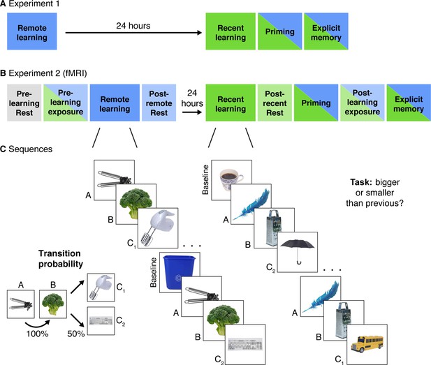
Experimental Design.
(A) Experiment 1 design. Participants completed two learning sessions separated by 24 hr (blue = remote, green = recent learning). (B) Experiment 2 design. The timing, instructions, and procedures for the learning and priming tasks were identical to Experiment 1, with a modified but conceptually similar explicit memory task. Participants also completed pre- and post-learning exposure scans where all objects from both learning sessions were presented in a randomly intermixed order. Three rest scans were added: a pre-learning scan at the start of Day 1, a post-remote learning scan on Day 1, and a post-recent learning scan on Day 2. (C) In each learning session, participants performed a cover task as they viewed objects embedded in triplets. All triplets were composed of two images that always appeared back-to-back (A and B) and two images that alternated following the AB pair (C1 and C2) with equal probability. Baseline objects were randomly inserted between triplets. Separate image sets were presented in each learning session. After the recent learning session, participants completed recognition priming and explicit memory tests over all objects intermixed from the two learning sessions (see Figure 2 for details of each test).
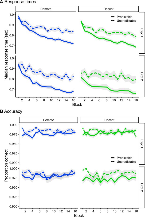
AB recognition priming and explicit integration.
(A) Median response times for predictable items (B and C) and unpredictable items (A and baseline) across learning. Error ribbons signify standard error of the mean (SEM) across participants. (B) Average proportion of correct size judgments for predictable items and unpredictable items across learning. Error ribbons signify SEM across participants. Plots can be reproduced with Figure 1—figure supplement 1—source data 1.
-
Figure 1—figure supplement 1—source data 1
Response times and accuracy during learning.
- https://cdn.elifesciences.org/articles/84359/elife-84359-fig1-figsupp1-data1-v1.csv
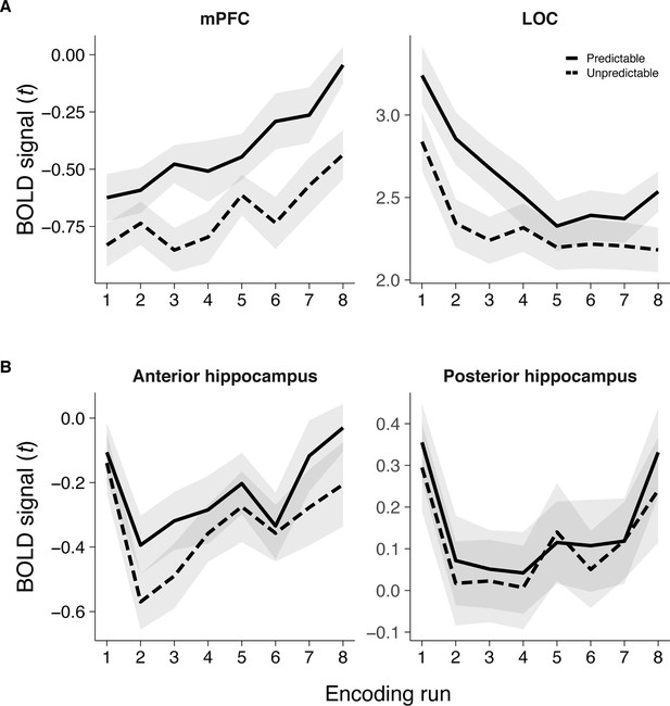
Average BOLD signal for predictable and unpredictable items across the eight learning runs, averaged over the recent and remote learning sessions.
(A) Average BOLD signal for mPFC and LOC, both of which were identified from whole brain contrasts comparing predictable and unpredictable items. (B) Average BOLD signal in anterior and posterior hippocampus, which were anatomically defined. Error ribbons indicate standard error of the mean (SEM) across participants. Plots can be reproduced with ‘Figure 1—figure supplement 2—source data 1'.
-
Figure 1—figure supplement 2—source data 1
Average BOLD signal during learning.
- https://cdn.elifesciences.org/articles/84359/elife-84359-fig1-figsupp2-data1-v1.csv
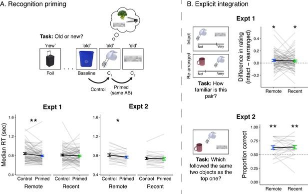
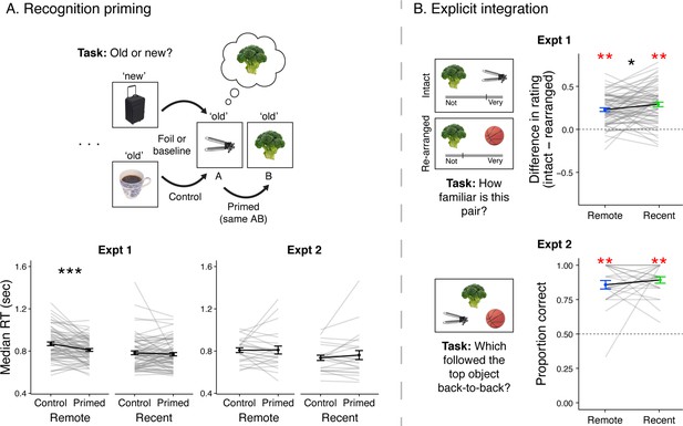
Recognition priming and explicit integration.
(A, top) Recognition priming design. Studied and new objects were presented pseudo-randomly such that each C2 object followed the C1 object from the same sequence, and the C1 object followed a baseline object from the same learning session. The behavioral integration of C1 and C2 was operationalized as the decrement in response time to C2 (preceded by C1) relative to C1 (preceded by a baseline object). (A, bottom) Recognition priming results. Statistics reflect results from trial-level mixed-effects models, but participants’ responses are aggregated to facilitate visualization of the effects. Black lines represent group averages. Gray lines represent median response times for each participant. Error bars indicate standard error of the mean (SEM) across participants. ** indicates p < 0.01; * indicates p < 0.05. (B, left) Explicit integration design. In Experiment 1, participants viewed intact and re-arranged pairs of C objects and rated their familiarity on a continuous scale from ‘Not familiar at all’ to ‘Very familiar’. All foils for re-arranged pairs were C objects from a different sequence learned in the same session. The average difference in rating for intact versus re-arranged pairs served as a measure of explicit integration across overlapping sequences. In Experiment 2, participants performed a 2-alternative forced choice (2AFC) task with a C object as the cue and were asked to choose which object followed the same pair of two objects as the cue. Foil images were C objects from a different sequence learned in the same session. (B, right) Explicit integration results. Black lines represent group averages. Gray lines represent participants. Error bars indicate standard error of the mean (SEM) across participants. Statistics reflect one-sample t-tests against chance performance. ** indicates p < 0.01; * indicates p < 0.05. Plots can be reproduced with data in ‘Figure 2—source data 1’ and ‘Figure 2—source data 2’.
-
Figure 2—source data 1
Recognition priming.
- https://cdn.elifesciences.org/articles/84359/elife-84359-fig2-data1-v1.csv
-
Figure 2—source data 2
Explicit integration.
- https://cdn.elifesciences.org/articles/84359/elife-84359-fig2-data2-v1.csv
Plots can be reproduced with ‘Figure 2—figure supplement 1—source data 1' and ‘Figure 2—figure supplement 1—source data 2'.
(A) AB priming results. All B items followed A items from the same sequence, analogous to the ordering of the C items. We compared response times (RTs) for B items (primed) to RTs to A items, which followed either a novel foil or an item from a different sequence (unprimed). We predicted that responses would be facilitated for primed items over unprimed items, and then this effect would be apparent immediately after learning. Note that due to constraints in pseudo-randomizing the order of these items, the comparison between A and B responses is not controlled for motor history, unlike the comparison between primed and unprimed C items. Black lines represent group averages. Gray lines represent participants. Error bars indicate standard error of the mean (SEM) across participants. Statistics reflect paired t-tests across primed and control trials. *** indicates p < 0.001. (A, bottom left) For Experiment 1, a trial-level mixed-effects linear model was computed with RT as the dependent variable and item (discrete: primed, control), day (discrete: recent, remote), and their interaction as predictors. This model revealed reliable effects of item (F(1, 1332.49) = 8.81, p = 0.003), and day (F(1, 65.72) = 20.66, p < 0.001), with no reliable interaction (F(1, 1332.64) = 2.27, p = 0.09). Comparisons of RTs by item separately for each day revealed that RTs were faster for primed items relative to unprimed items for the remotely learned items (F(1, 662.29) = 10.21, p = 0.001) but not recently learned items (F(1, 672.0) = 0.94, p = 0.33). In Experiment 2, the same day by item model revealed no reliable effect of item (F(1, 467.00) = 0.03, p = 0.87), a reliable effect of day (F(1, 20.95) = 6.87, p = 0.02) reflecting slower RTs for items from remotely learned sequences, and no interaction (F(1, 467.52) = 0.37, p = 0.54). There were no reliable differences in RT for primed and unprimed items for sequences from either session (both F’s < 0.30, both p’s > 0.59). (A, bottom right) In Experiment 2, the same day by item model revealed no reliable effect of item (F(1, 467.00) = 0.03, p = 0.87), a reliable effect of day (F(1, 20.95) = 6.87, p = 0.02) reflecting slower RTs for items from remotely learned sequences, and no interaction (F(1, 467.52) = 0.37, p = 0.54). There were no reliable differences in RT for primed and unprimed items for sequences from either session (both F’s < 0.30, both p’s > 0.59). (B) Explicit integration of AB pairs. In Experiment 1, participants viewed pairs of A and B items that either came from the same sequence (Intact) or different ones (Re-arranged) during learning. They rated the familiarity of these pairs on a sliding scale exactly as for C items. In Experiment 2, we tested participants’ memory for AB pairs with a 2-alternative forced choice (2AFC) task with either the A or B item as the cue, the other item as the target, and a foil matching the status of the target item (A or B from another sequence). Black lines represent group averages. Gray lines represent participants. Error bars indicate standard error of the mean (SEM) across participants. Statistics reflect one-sample t-tests against chance performance. *** indicates p < 0.001. (B top right) Accuracy was reliably above chance (remote: mean = 0.229, standard deviation (SD) = 0.176, t(70) = 11.0, p < 0.001; recent: mean = 0.291, SD = 0.218, t(70) = 11.2, p < 0.001) with reliably better memory for pairs from the recent session over the remote session (t(70) = 2.42, p = 0.02). (B bottom right) Average accuracy was above chance for items learned remotely (mean = 0.86, SD = 0.152, t(23) = 11.5, p < 0.001) and recently (mean = 0.892, SD = 0.114, t(23) = 16.9, p < 0.001) with no difference in accuracy as a function of the two learning sessions (t(23) = −0.84, p = 0.41).
-
Figure 2—figure supplement 1—source data 1
AB recognition priming.
- https://cdn.elifesciences.org/articles/84359/elife-84359-fig2-figsupp1-data1-v1.csv
-
Figure 2—figure supplement 1—source data 2
AB explicit integration.
- https://cdn.elifesciences.org/articles/84359/elife-84359-fig2-figsupp1-data2-v1.csv
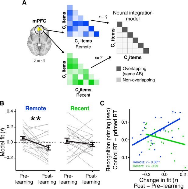
Learning- and consolidation-dependent changes in mPFC neural integration.
(A) Analysis approach for exposure scans. Vectors of multi-variate activation were extracted from a medial prefrontal cortex (mPFC) region of interest (ROI) for each C object and correlated with vectors for all C objects from overlapping and distinct sequences viewed in the same learning session (recent and remote). These correlation matrices were correlated with an ‘integration model’ reflecting greater similarity for C objects belonging to an overlapping sequence (i.e. objects that followed the same AB sequence). This analysis was repeated for both exposure phases and subtracted (post- minus pre-learning exposure) to create change scores. (B) Average fit to the integration model for the pre- and post-learning exposure phases in mPFC, separately for recently and remotely learned sequences. Values <0 indicate a worse fit to the model, meaning more differentiation between C objects from overlapping sequences relative to C objects from different sequences (see also Figure 3—figure supplement 1). Gray lines indicate participants. Black line indicates group average. Error bars reflect standard error of the mean (SEM). ** indicates p < 0.01. (C) Correlation between the average change in the fit to the integration model in mPFC and average recognition priming across participants, separately for recent and remote learning. Dots indicate participants. Lines indicate line of best fit. Plots can be reproduced with ‘Figure 3—source data 1.csv’ and ‘Figure 3—source data 2.csv’.
-
Figure 3—source data 1
mPFC fit to neural integration model.
- https://cdn.elifesciences.org/articles/84359/elife-84359-fig3-data1-v1.csv
-
Figure 3—source data 2
mPFC neural integration related to recognition priming.
- https://cdn.elifesciences.org/articles/84359/elife-84359-fig3-data2-v1.csv
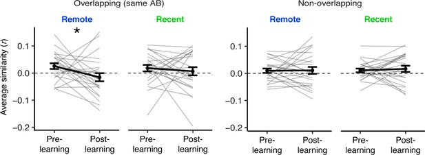
Average similarity across C1 and C2 items in overlapping sequences (left) and non-overlapping sequences (right), separately for the pre- and post-learning exposure phases and for recent and remotely learned sequences.
Gray lines indicate participants. Black line indicates group average. Error bars reflect standard error of the mean (SEM). Black asterisks indicate a two-tailed paired t-test across pre- and post-learning similarity. * indicates p < 0.05. Plots can be reproduced with ‘Figure 3—figure supplement 1—source data 1’.
-
Figure 3—figure supplement 1—source data 1
mPFC similarity for overlapping and non-overlapping sequences.
- https://cdn.elifesciences.org/articles/84359/elife-84359-fig3-figsupp1-data1-v1.csv
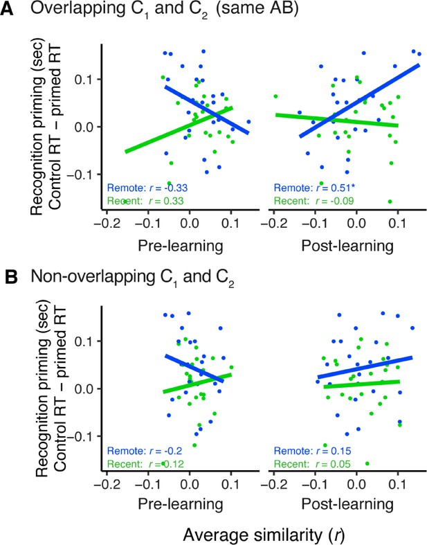
mPFC similarity related to recognition priming.
Correlation between each participant’s recognition priming with their average similarity in medial prefrontal cortex (mPFC) across overlapping C1 and C2 items (A) and non-overlapping C1 and C2 items (B). This was conducted separately for sequences in the recent (green) and remote (blue) learning sessions. * indicates p < 0.05. Dots indicate participants. Lines indicate line of best fit. Plots can be reproduced with ‘Figure 3—figure supplement 2—source data 1'.
-
Figure 3—figure supplement 2—source data 1
mPFC similarity related to recognition priming.
- https://cdn.elifesciences.org/articles/84359/elife-84359-fig3-figsupp2-data1-v1.csv
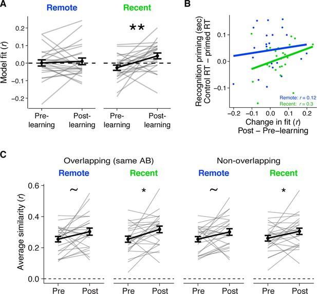
Neural integration in LOC.
(A) Average fit of LOC patterns to the neural integration model, separately for post- and pre-learning exposure phases and for pairs of C items that were in recently and remotely learned sequences. Values >0 indicate a better fit to the model after learning, meaning higher similarity of C items from overlapping sequences relative to C items from different sequences. Gray lines indicate participants. Black line indicates group average. Error bars reflect standard error of the mean (SEM). Black asterisks indicate a two-tailed paired t-test across learning sessions. ** indicates p < 0.01. (B) Correlation between the average change in LOC model fit and recognition priming across participants, separately for recent and remote learning. Dots indicate participants. Lines indicate best fit. (C) Average similarity across C1 and C2 items in overlapping sequences (left) and non-overlapping sequences (right), separately for the pre- and post-learning exposure phases and for recent and remotely learned sequences. Black asterisks indicate a two-tailed paired t-test across pre- and post-learning similarity. * indicates p < 0.05; ~ indicates p < 0.10. Plots can be reproduced with ‘Figure 3—figure supplement 3—source data 1–3'.
-
Figure 3—figure supplement 3—source data 1
LOC fit to neural integration model.
- https://cdn.elifesciences.org/articles/84359/elife-84359-fig3-figsupp3-data1-v1.csv
-
Figure 3—figure supplement 3—source data 2
LOC neural integration related to recognition priming.
- https://cdn.elifesciences.org/articles/84359/elife-84359-fig3-figsupp3-data2-v1.csv
-
Figure 3—figure supplement 3—source data 3
LOC similarity for overlapping and non-overlapping sequences.
- https://cdn.elifesciences.org/articles/84359/elife-84359-fig3-figsupp3-data3-v1.csv
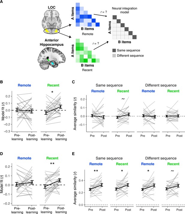
Neural integration of A and B items.
(A) To investigate whether patterns of A and B items became more integrated over learning and consolidation, we presented all A and B items in the pre- and post-learning exposure scans, intermixed with all C items. We quantified the extent of their neural integration by extracting patterns of BOLD signal for each item and compiling the correlation between all patterns into a correlation matrix with A items in rows and B items in columns. We created separate matrices for items learned in sequences recently or remotely. We then compared each matrix against a model matrix postulating greater similarity between A and B items from overlapping sequences, i.e. items repeated back-to-back 100% of the time, relative to similarity between A and B items from different sequences. (B) Model fits for anterior hippocampus (recent: t(23) = 2.56, p = 0.017, Bonferroni-corrected p = 0.051); remote: t(23) = −0.50, p = 0.62). (C) Average similarity in the anterior hippocampus for AB pairs in the same (left) and different (right) sequences. (D) Model fits for LOC (recent: t(23) = 2.84, p = 0.009, Bonferroni-corrected p = 0.027; remote: t(23) = 0.74, p = 0.47. (E) Average similarity in LOC for AB pairs in the same (left) and different (right) sequences. (B, D) Values >0 indicate a better fit to the model, reflecting greater integration of A and B items from overlapping sequences relative to A and B items from different sequences. These changes were not related to the extent of recognition priming across sequences (all r’s < 0.21, all p’s > 0.15). (B–E) Gray lines indicate participants. Black line indicates group average. Error bars reflect standard error of the mean (SEM). Black asterisks indicate a two-tailed paired t-test across exposure scans. ** indicates p < 0.01; * indicates p < 0.05; ~indicates p < 0.01. Plots can be reproduced with ‘Figure 3—figure supplement 4—source data 1–4'.
-
Figure 3—figure supplement 4—source data 1
Neural integration of A and B in anterior hippocampus.
- https://cdn.elifesciences.org/articles/84359/elife-84359-fig3-figsupp4-data1-v1.csv
-
Figure 3—figure supplement 4—source data 2
Neural similarity for overlapping and non-overlapping A and B sequences in anterior hippocampus.
- https://cdn.elifesciences.org/articles/84359/elife-84359-fig3-figsupp4-data2-v1.csv
-
Figure 3—figure supplement 4—source data 3
Neural integration of A and B in LOC.
- https://cdn.elifesciences.org/articles/84359/elife-84359-fig3-figsupp4-data3-v1.csv
-
Figure 3—figure supplement 4—source data 4
Neural similarity for overlapping and non-overlapping A and B sequences in LOC.
- https://cdn.elifesciences.org/articles/84359/elife-84359-fig3-figsupp4-data4-v1.csv
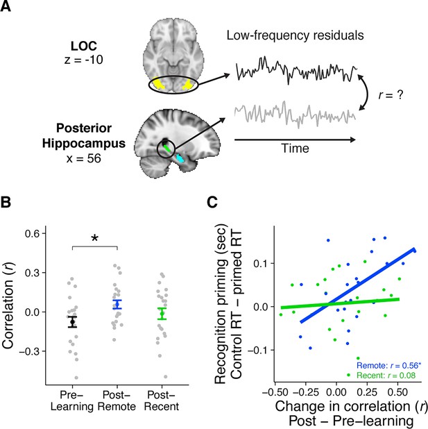
Rest connectivity between LOC and posterior hippocampus.
(A) Analytic approach for rest scans. Rest scans were preprocessed, stripped of nuisance signals, and band-pass filtered. The mean residual signal was extracted from the posterior hippocampus and LOC for each volume of each scan. Rest connectivity was measured by correlating their mean time courses. (B) Average rest connectivity between LOC and posterior hippocampus. Gray dots indicate participants. Black, blue, and green dots indicate group averages. Error bars reflect standard error of the mean (SEM). * indicates p < 0.05. (C) Correlation between the change in LOC—posterior hippocampal rest connectivity and average recognition priming across participants, separately for recent and remote learning. Dots indicate participants. Lines indicate best fit. Plots can be reproduced with ‘Figure 4—source data 1.csv’ and ‘Figure 4—source data 2.csv’.
-
Figure 4—source data 1
Rest connectivity between LOC and posterior hippocampus.
- https://cdn.elifesciences.org/articles/84359/elife-84359-fig4-data1-v1.csv
-
Figure 4—source data 2
Rest connectivity between LOC and posterior hippocampus related to recognition priming.
- https://cdn.elifesciences.org/articles/84359/elife-84359-fig4-data2-v1.csv
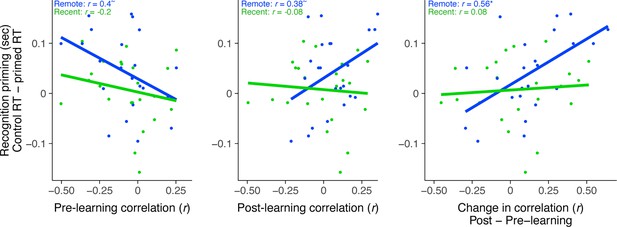
Rest connectivity between LOC and posterior hippocampus related to recognition priming, separately for pre- and post-learning rest scans.
Correlation between LOC connectivity with posterior hippocampus and recognition priming across participants, separately for recent and remote learning. Analysis conducted separately for pre-learning rest, post-learning rest, and the change (post- minus pre-learning) which is a copy of Figure 4C included for ease of comparison. Dots indicate participants. Lines indicate line of best fit. Plots can be reproduced with ‘Figure 4—figure supplement 1—source data 1'.
-
Figure 4—figure supplement 1—source data 1
Rest connectivity between LOC and posterior hippocampus related to recognition priming, separately for pre- and post-learning rest scans.
- https://cdn.elifesciences.org/articles/84359/elife-84359-fig4-figsupp1-data1-v1.csv
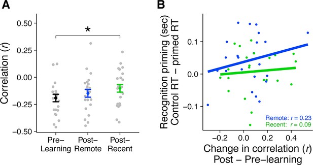
Rest connectivity between LOC and mPFC.
(A) Average rest connectivity between LOC and medial prefrontal cortex (mPFC). Gray dots indicate participants. Black, blue and green dots indicate group averages. Error bars reflect standard error of the mean (SEM). * indicates p < 0.05. (B) Correlation between the average change in LOC–mPFC connectivity and recognition priming across participants, separately for recent and remote learning. Dots indicate participants. Lines indicate line of best fit. Plots can be reproduced with ‘Figure 4—figure supplement 2—source data 1 and 2'.
-
Figure 4—figure supplement 2—source data 1
Rest connectivity between LOC and mPFC.
- https://cdn.elifesciences.org/articles/84359/elife-84359-fig4-figsupp2-data1-v1.csv
-
Figure 4—figure supplement 2—source data 2
Rest connectivity between LOC and mPFC, related to recognition priming.
- https://cdn.elifesciences.org/articles/84359/elife-84359-fig4-figsupp2-data2-v1.csv
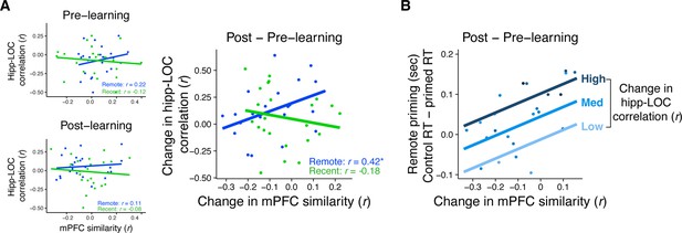
Relationship between mPFC similarity, rest connectivity, and priming.
(A) Correlation between medial prefrontal cortex (mPFC) similarity and rest connectivity between posterior hippocampus and LOC across participants, separately for pre- and post-learning connectivity and pre- and post-learning similarity in mPFC (left) and for the change in connectivity and similarity (post- minus pre-learning; right). Dots represent participants and lines represent model fit. * indicates p < 0.05. (B) Visualization of multiple linear regression predicting recognition priming for the remotely learned sequences. Each dot is a participant. Color indicates the magnitude of the change in rest connectivity between posterior hippocampus and LOC. Lines represent fits of the model at different magnitudes of rest connectivity. Plots can be reproduced with Figure 5—source data 1–3.
-
Figure 5—source data 1
Relationship between mPFC similarity and rest connectivity, separately for pre- and post-learning rest scans.
- https://cdn.elifesciences.org/articles/84359/elife-84359-fig5-data1-v1.csv
-
Figure 5—source data 2
Relationship between change in mPFC similarity and change in rest connectivity.
- https://cdn.elifesciences.org/articles/84359/elife-84359-fig5-data2-v1.csv
-
Figure 5—source data 3
Relationship between mPFC similarity, rest similarity, and recognition priming.
- https://cdn.elifesciences.org/articles/84359/elife-84359-fig5-data3-v1.csv
Tables
Mean (SD) transition probabilities for all objects during.
(A) Learning in both experiments, (B) recognition priming in both experiments, (C) the first exposure scan, and (D) the second exposure scan. As a reminder, the pre- and post-learning exposure phases were divided into two scans, one that comprised A, C1, and baseline objects, and one that only comprised B, C2, and baseline objects (see Methods). Italicized values indicate transition probabilities that additionally are specific to objects from the same sequence. For example, during learning, not only does a B object follow every A object, but the same B object follows the same A object 100% of the time. In contrast, baseline objects are always followed by A objects, but the specific objects vary.
| A | Follows | ||||||
| A | B | C1 | C2 | Base | |||
| Precedes | A | 0 (0) | 1 (0) | 0 (0) | 0 (0) | 0 (0) | |
| B | 0 (0) | 0 (0) | 0.5 (0) | 0.5 (0) | 0 (0) | ||
| C1 | 0.5 (0.04) | 0 (0) | 0 (0) | 0 (0) | 0.5 (0.04) | ||
| C2 | 0.5 (0.04) | 0 (0) | 0 (0) | 0 (0) | 0.5 (0.04) | ||
| Base | 1 (0) | 0 (0) | 0 (0) | 0 (0) | 0 (0) | ||
| B | Follows | ||||||
| A | B | C1 | C2 | Base | Foil | ||
| Precedes | A | 0 (0) | 1 (0) | 0 (0) | 0 (0) | 0 (0) | 0 (0) |
| B | 0.11 (0.08) | 0 (0) | 0 (0) | 0 (0) | 0.18 (0.10) | 0.71 (0.11) | |
| C1 | 0 (0) | 0 (0) | 0 (0) | 1 (0) | 0 (0) | 0 (0) | |
| C2 | 0.15 (0.10) | 0 (0) | 0 (0) | 0 (0) | 0 (0) | 0.84 (10) | |
| Base | 0 (0) | 0 (0) | 1 (0) | 0 (0) | 0 (0) | 0 (0) | |
| Foil | 0.22 (0.03) | 0 (0) | 0 (0) | 0 (0) | 0.25 (0.03) | 0.52 (0.03) | |
| C | Follows | ||||||
| A | C1 | Base | |||||
| Precedes | A | 0.39 (0.05) | 0.40 (0.06) | 0.21 (0.04) | |||
| C1 | 0.39 (0.06) | 0.42 (0.05) | 0.19 (0.05) | ||||
| Base | 0.43 (0.08) | 0.37 (0.07) | 0.20 (0.06) | ||||
| D | Follows | ||||||
| B | C2 | Base | |||||
| Precedes | B | 0.39 (0.05) | 0.39 (0.05) | 0.21 (0.04) | |||
| C2 | 0.41 (0.04) | 0.39 (0.05) | 0.21 (0.04) | ||||
| Base | 0.40 (0.08) | 0.44 (0.08) | 0.16 (0.05) | ||||
R and L indicate right and left hemispheres.
Extent is size of the clusters in voxels. x, y, and z coordinates indicate the center of gravity in MNI space (mm). p corresponds to corrected significance of cluster. * indicates clusters used for ROIs.
| Region | Extent | x | y | z | p |
|---|---|---|---|---|---|
| Predictable > unpredictable | |||||
| *R Parahippocampal, lateral occipital cortex | 4644 | 28.1 | −77.8 | −3.82 | <0.001 |
| *L Parahippocampal, lateral occipital cortex | 2623 | −29.1 | −80.3 | −5.08 | <0.001 |
| L Angular gyrus, central opercular cortex | 1246 | −52.1 | −43.3 | 27.1 | <0.001 |
| * Medial prefrontal cortex, frontal pole | 1195 | −2.43 | 54.5 | 4.31 | <0.001 |
| R Angular gyrus, middle temporal gyrus | 911 | 62.2 | −41.2 | 10.1 | <0.001 |
| Posterior medial cortex | 675 | −0.133 | −47.5 | 34 | <0.001 |
| Middle temporal gyrus, posterior | 372 | −56.2 | −24.9 | −5.67 | <0.001 |
| Posterior cingulate gyrus | 308 | 1.43 | −21 | 39.6 | <0.001 |
| R Parietal operculum cortex | 217 | 59.7 | −24.8 | 21.1 | <0.001 |
| R Inferior frontal gyrus | 197 | 55.2 | 31.3 | −1.84 | 0.001 |
| L Putamen | 168 | −28.5 | −10.8 | 5.01 | 0.003 |
| L Middle temporal gyrus, anterior | 142 | −51.6 | −1.3 | −23.9 | 0.008 |
| R Frontal Pole | 98 | 16 | 53.2 | 28.1 | 0.04 |
| Unpredictable > predictable | |||||
| L Insula, inferior and middle frontal gyrus | 1788 | −39.7 | 20.1 | 12 | <0.001 |
| R Insula, inferior frontal gyrus | 802 | 36.4 | 19.8 | 4.41 | <0.001 |
| L Supramarginal gyrus | 252 | −39.4 | −43.7 | 43.1 | <0.001 |
| Paracingulate cortex | 221 | −0.922 | 25.8 | 36.4 | <0.001 |
| R Middle frontal gyrus | 199 | 44.3 | 33.7 | 21.4 | 0.001 |
| L Inferior temporal gyrus | 142 | −52.7 | −55.2 | −10.6 | 0.008 |
| L Superior lateral occipital cortex | 98 | −22.6 | −65.7 | 38.5 | 0.04 |


