Leveraging place field repetition to understand positional versus nonpositional inputs to hippocampal field CA1
- Krieger Mind/Brain Institute, Johns Hopkins University, United States
- Solomon H. Snyder Department of Neuroscience, Johns Hopkins University School of Medicine, United States
- Kavli Neuroscience Discovery Institute, Johns Hopkins University, United States
Figures
Figure 1 with 9 supplements
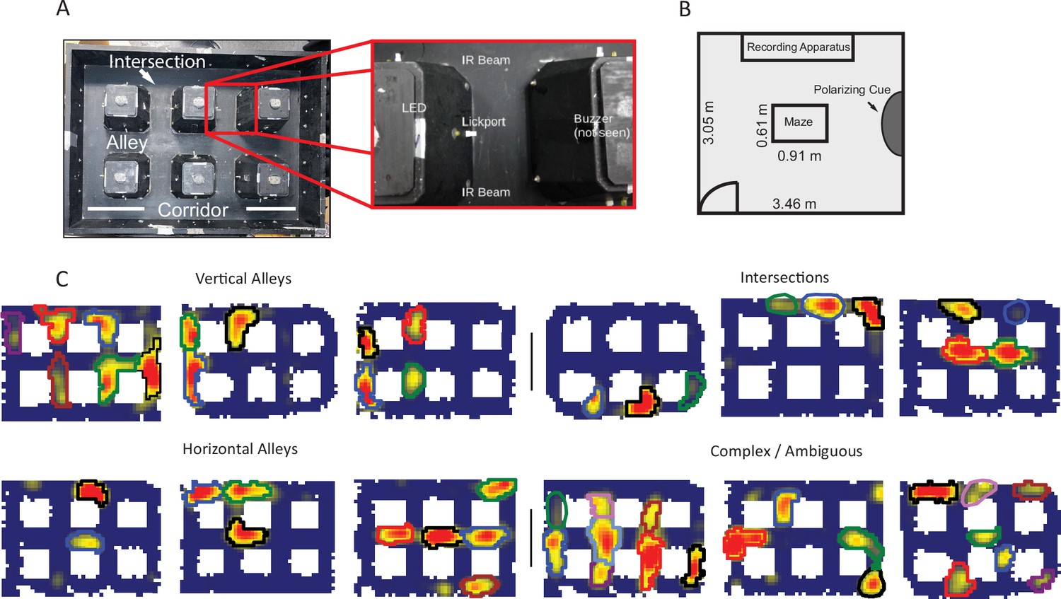
Apparatus and examples of place field repetition.
(A) Left, top-down view of city-block maze. Perimeter walls (15.2 cm high) enclose an area 60.96×91.44 cm2. Six square obstacles (19.1×19.1 cm2, 15.2 cm tall) define 17 alleys in their interstitial spaces along with 12 intersections. Track regions were defined as vertical alleys (oriented north-south), horizontal alleys (oriented east-west), or intersections. Right, enhancement showing an individual alley. An IR emitter and detector pair was affixed to either entrance of the alley. In the center of the alley was a lickport with a visible light LED above. A buzzer was placed under each alley. Lickports here have been extended to make them more visible. (B) Schematic of recording room and behavioral apparatus. The city-block maze was in the same room as the recording apparatus. A black, floor-to-wall curtain that was gathered together, forming a band along the east wall, served as a polarizing cue. (C) Examples of repeating fields grouped into four subjective categories: repeating in vertical alleys, repeating in horizontal alleys, repeating in intersections, and complicated or ambiguous patterns of repetition. Spatial bins from off-track sampling were removed from these figures and from quantitative analyses of the place fields. Each identified subfield is outlined in a separate color.
Figure 1—figure supplement 1
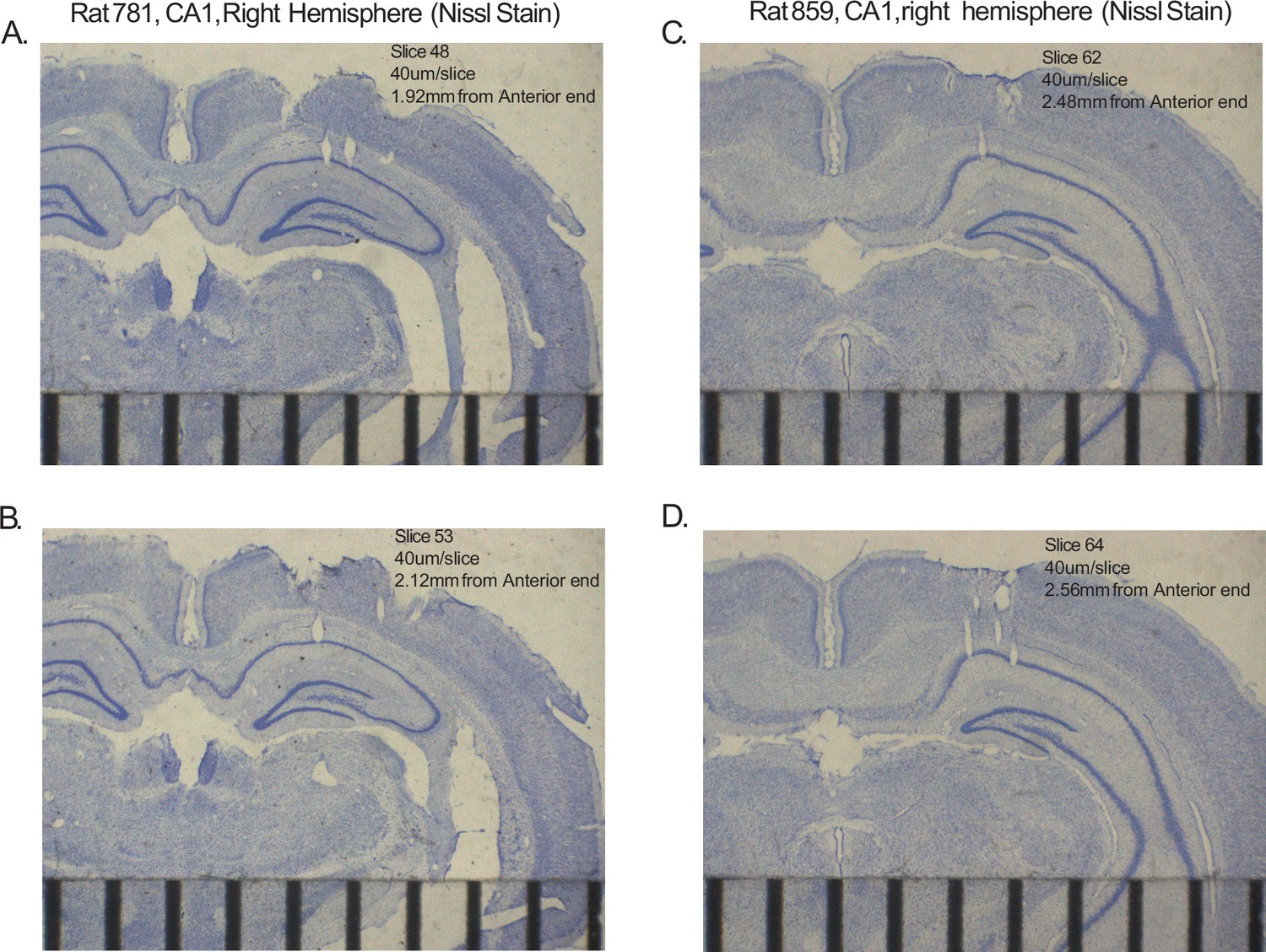
Histology from representative animals.
All panels are 40 μm slices, Nissl stained from the right hemisphere CA1. Scale bars indicate mm. Tears in/near CA1 layer indicate location of tetrode tracks. Ruler at bottom of figures shows mm gradations. (A) Two tetrode tracks are visible in intermediate (along the transverse axis) CA1 at 1.92 mm along the anterior-posterior axis (A-P axis), starting from the septal pole of the hippocampus. (B) One tetrode track visible in intermediate CA1 at 2.12 mm A-P. (C) One tetrode track is visible in distal CA1 at 2.48 mm along the A-P axis. (D) Three tetrode tracks are visible in/near distal CA1 at 2.56 mm A-P.
Figure 1—figure supplement 2
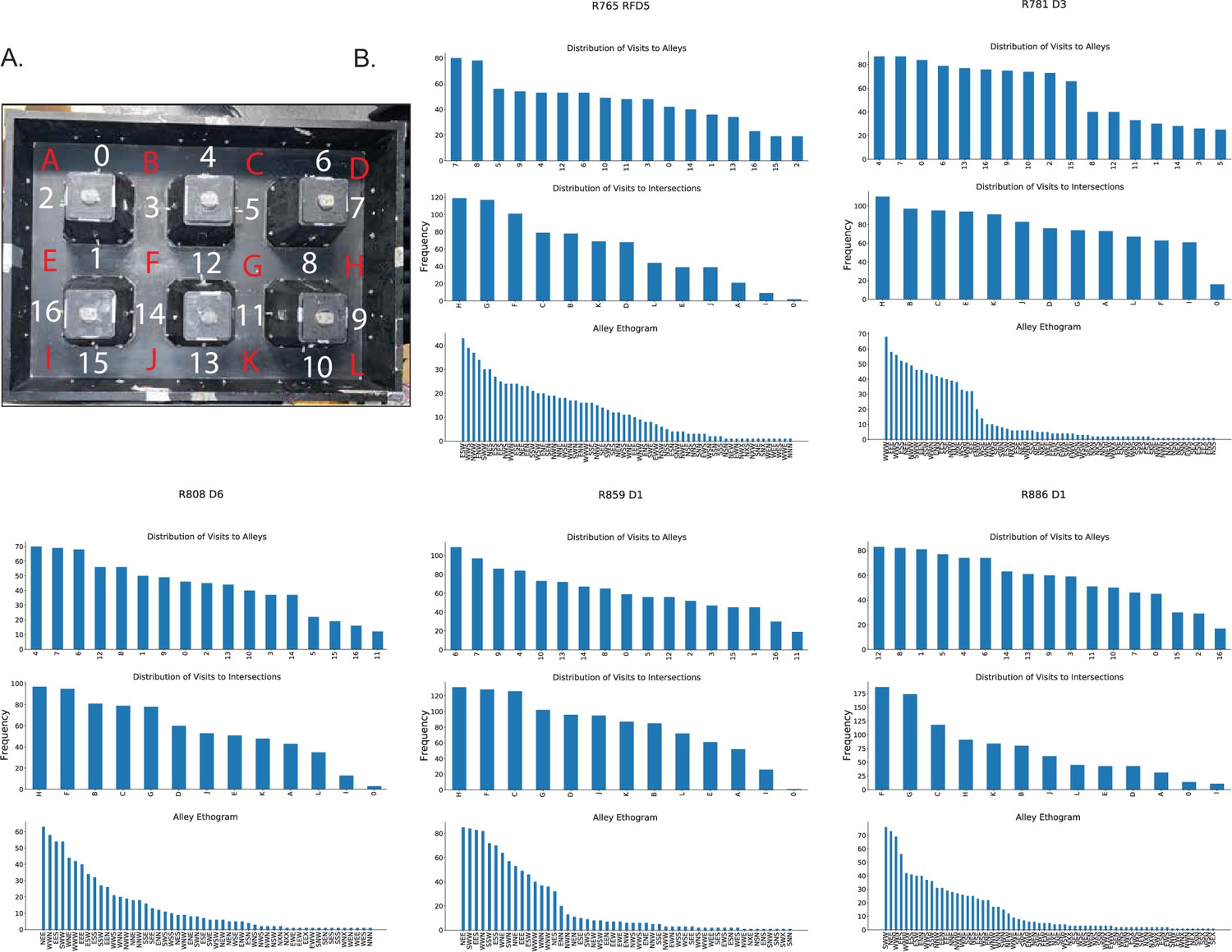
Behavioral sampling.
(A) Photograph of city-block maze annotated with region labels. Alleys denoted by numbers, intersections by letters. (B) Behavioral sampling of alleys and intersections for 1 day of recording of each rat. Top, histogram of visit counts to each alley. Middle, histogram of visit count to each intersection. Bottom, histogram of routes through alleys. A route is defined as a sequence of headings through a field: previous direction, current direction, next direction. For example, a label ‘NES’ corresponds to a journey through the alley where the direction prior to turning into the alley was north, the path through the alley was east, and the turn out of the alley was south.
Figure 1—figure supplement 3
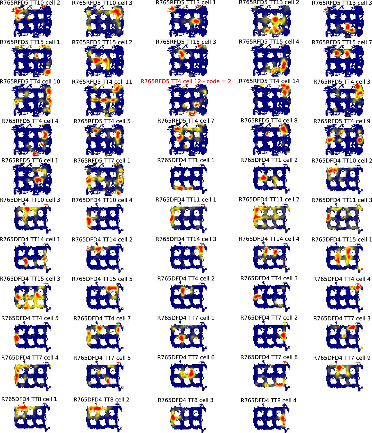
All ratemaps for R765.
Each panel is the ratemap from a well-isolated neuron with on-track firing. No pass-sampling thresholds have been applied. Unlike the ratemaps shown in the main text, these ratemaps include the firing of the cell when the rat’s head was outside the boundaries of the track, when it was rearing and investigating the outside environment rather than performing the task. The inclusion of this off-track behavior accounts for the ragged edges of the ratemaps. The off-track activity was not analyzed, due to the variability in this behavior across rats and across locations within rats. Instead, analysis was restricted to the alleys and intersections of the maze. Note the prevalence of cells that had multiple place fields in the alleys and intersections. Neurons excluded from further analysis because they were classified as interneurons or did not have place fields that are indicated by red titles and a numeric code detailing why they were excluded. The code legend is as follows: (1) Place field detection algorithm did not detect any fields (i.e. firing hotspots too small and/or low rate). (2) Manual exclusion: Most firing rate off-track, often ‘scanning’ firing. (3) Manual exclusion: Firing mostly occurred as a burst when animal was placed on or taken off the track. (4) Manual exclusion: Algorithm’s field identification and partition did not match experimenter’s visual inspection. (5) Manual exclusion: Algorithm detected fields but there was excessive out-of-field firing.
Figure 1—figure supplement 4
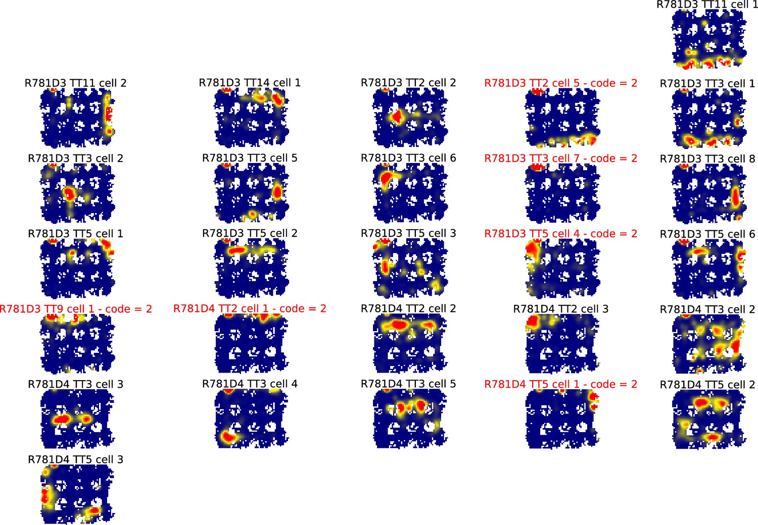
All ratemaps for R781.
Each panel is the ratemap from a well-isolated neuron with on-track firing. No pass-sampling thresholds have been applied. Unlike the ratemaps shown in the main text, these ratemaps include the firing of the cell when the rat’s head was outside the boundaries of the track, when it was rearing and investigating the outside environment rather than performing the task. The inclusion of this off-track behavior accounts for the ragged edges of the ratemaps. The off-track activity was not analyzed, due to the variability in this behavior across rats and across locations within rats. Instead, analysis was restricted to the alleys and intersections of the maze. Note the prevalence of cells that had multiple place fields in the alleys and intersections. Neurons excluded from further analysis because they were classified as interneurons or did not have place fields that are indicated by red titles and a numeric code detailing why they were excluded. The code legend is as follows: (1) Place field detection algorithm did not detect any fields (i.e. firing hotspots too small and/or low rate). (2) Manual exclusion: Most firing rate off-track, often ‘scanning’ firing. (3) Manual exclusion: Firing mostly occurred as a burst when animal was placed on or taken off the track. (4) Manual exclusion: Algorithm’s field identification and partition did not match experimenter’s visual inspection. (5) Manual exclusion: Algorithm detected fields but there was excessive out-of-field firing.
Figure 1—figure supplement 5
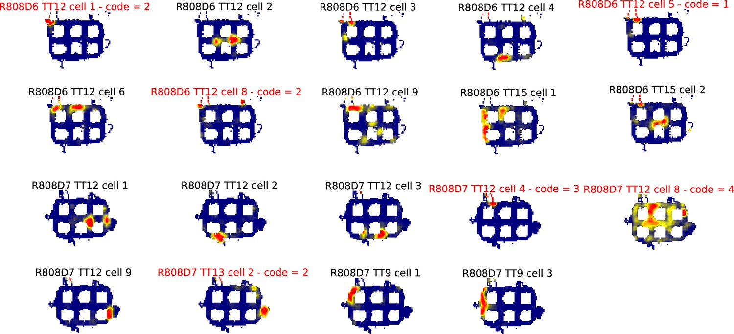
All ratemaps for R808.
Each panel is the ratemap from a well-isolated neuron with on-track firing. No pass-sampling thresholds have been applied. Unlike the ratemaps shown in the main text, these ratemaps include the firing of the cell when the rat’s head was outside the boundaries of the track, when it was rearing and investigating the outside environment rather than performing the task. The inclusion of this off-track behavior accounts for the ragged edges of the ratemaps. The off-track activity was not analyzed, due to the variability in this behavior across rats and across locations within rats. Instead, analysis was restricted to the alleys and intersections of the maze. Note the prevalence of cells that had multiple place fields in the alleys and intersections. Neurons excluded from further analysis because they were classified as interneurons or did not have place fields that are indicated by red titles and a numeric code detailing why they were excluded. The code legend is as follows: (1) Place field detection algorithm did not detect any fields (i.e. firing hotspots too small and/or low rate). (2) Manual exclusion: Most firing rate off-track, often ‘scanning’ firing. (3) Manual exclusion: Firing mostly occurred as a burst when animal was placed on or taken off the track. (4) Manual exclusion: Algorithm’s field identification and partition did not match experimenter’s visual inspection. (5) Manual exclusion: Algorithm detected fields but there was excessive out-of-field firing.
Figure 1—figure supplement 6
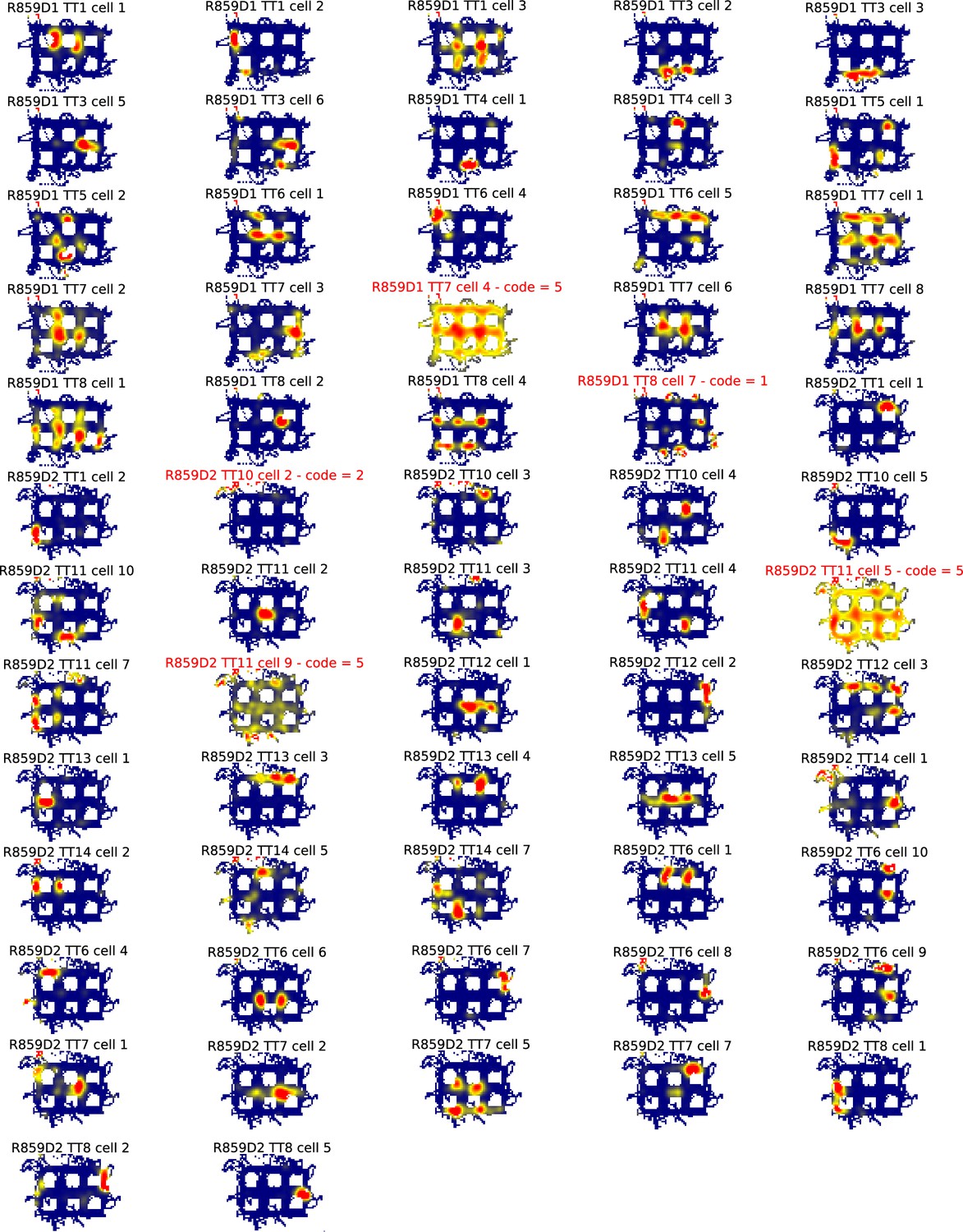
All ratemaps for R859.
Each panel is the ratemap from a well-isolated neuron with on-track firing. No pass-sampling thresholds have been applied. Unlike the ratemaps shown in the main text, these ratemaps include the firing of the cell when the rat’s head was outside the boundaries of the track, when it was rearing and investigating the outside environment rather than performing the task. The inclusion of this off-track behavior accounts for the ragged edges of the ratemaps. The off-track activity was not analyzed, due to the variability in this behavior across rats and across locations within rats. Instead, analysis was restricted to the alleys and intersections of the maze. Note the prevalence of cells that had multiple place fields in the alleys and intersections. Neurons excluded from further analysis because they were classified as interneurons or did not have place fields that are indicated by red titles and a numeric code detailing why they were excluded. The code legend is as follows: (1) Place field detection algorithm did not detect any fields (i.e. firing hotspots too small and/or low rate). (2) Manual exclusion: Most firing rate off-track, often ‘scanning’ firing. (3) Manual exclusion: Firing mostly occurred as a burst when animal was placed on or taken off the track. (4) Manual exclusion: Algorithm’s field identification and partition did not match experimenter’s visual inspection. (5) Manual exclusion: Algorithm detected fields but there was excessive out-of-field firing.
Figure 1—figure supplement 7
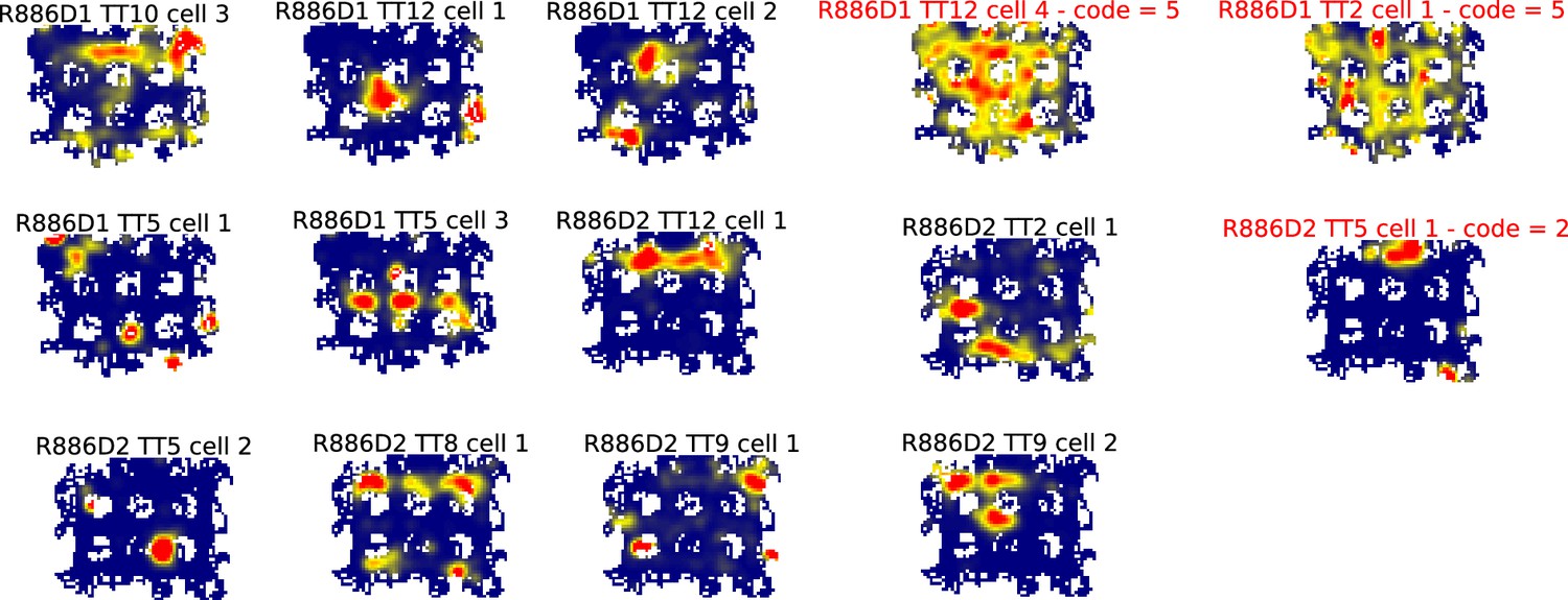
All ratemaps for R886.
Each panel is the ratemap from a well-isolated neuron with on-track firing. No pass-sampling thresholds have been applied. Unlike the ratemaps shown in the main text, these ratemaps include the firing of the cell when the rat’s head was outside the boundaries of the track, when it was rearing and investigating the outside environment rather than performing the task. The inclusion of this off-track behavior accounts for the ragged edges of the ratemaps. The off-track activity was not analyzed, due to the variability in this behavior across rats and across locations within rats. Instead, analysis was restricted to the alleys and intersections of the maze. Note the prevalence of cells that had multiple place fields in the alleys and intersections. Neurons excluded from further analysis because they were classified as interneurons or did not have place fields that are indicated by red titles and a numeric code detailing why they were excluded. The code legend is as follows: (1) Place field detection algorithm did not detect any fields (i.e. firing hotspots too small and/or low rate). (2) Manual exclusion: Most firing rate off-track, often ‘scanning’ firing. (3) Manual exclusion: Firing mostly occurred as a burst when animal was placed on or taken off the track. (4) Manual exclusion: Algorithm’s field identification and partition did not match experimenter’s visual inspection. (5) Manual exclusion: Algorithm detected fields but there was excessive out-of-field firing.
Figure 1—figure supplement 8
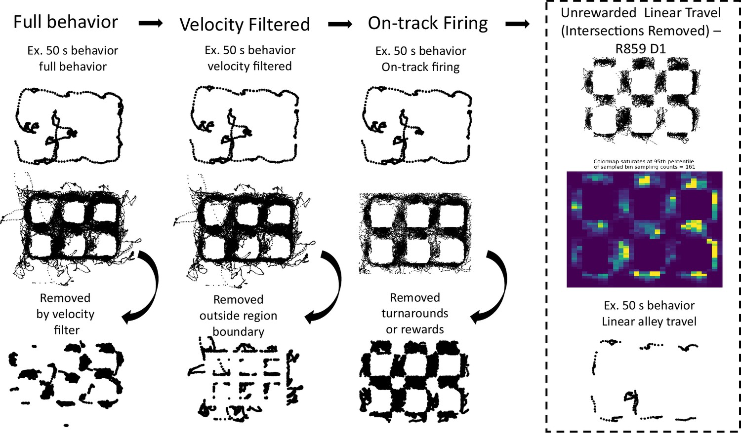
Behavioral processing pipeline.
A schematic of the general preprocessing steps applied to behavioral data from one representative dataset. In each column, the top row shows an example snippet of the behavior present at that step, the middle row shows the data present at that step of processing, and the bottom row shows the behavior that is excluded from that step to the next. The right-most column (enclosed in dashed lines) shows the final behavior that is used for analysis.
Figure 1—figure supplement 9
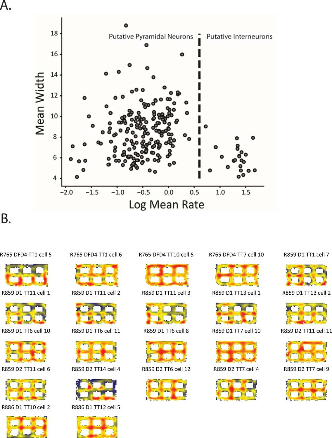
Putative interneurons.
(A) Putative excitatory neurons and inhibitory neurons (i.e. interneurons) were operationally separated on the basis of the log mean firing rate versus the mean waveform width. Putative excitatory cells and interneurons could be separated by a simple firing rate threshold (dashed line). (B) Ratemaps of the neurons in the cluster to the right of the dashed line in (A). Qualitatively, some neurons displayed local firing fields at regular locations but the small number of recorded interneurons limited the inferences one could make by performing statistical tests on the population.
Figure 2

Characterization of repetition.
(A) The frequency of place field repetition across days and rats as defined operationally (two or more fields in a common location). Each bar shows the proportion of well-isolated cells with on-track firing that was repeating, from ten datasets across five rats. (B) The distribution of number of fields within repeating cells. Repeating cells had between two and seven detected fields, with half of cells displaying four or more fields. (C) The orientation bias among repeating fields in alleys. Cells were assigned an ‘orientation bias score’ by taking the ratio between the maximum number of fields sharing a common orientation and the total number of fields. (D) To quantify repetition, the orientation alignment score (OAS) was defined. The metric first defines the degree of alignment of the fields of a cell, and then expresses that as a percent along the range of possible alignments for that given the number of fields the cell had (see Materials and methods). The y-axis indicates frequency of shuffles of the entire population that had the average OAS indicated on the x-axis. The mean of the population 0.71 (red) was greater than the 95th percentile of a shuffle distribution (0.64, black).
Figure 3 with 2 supplements
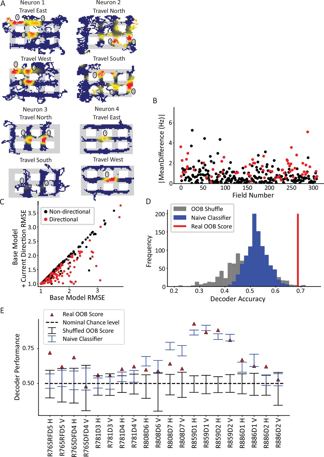
Directionality of place fields in the city-block maze.
(A) Examples of directional place fields. Only unrewarded, straight-through traversals were included for these ratemaps and subsequent analyses. Top left, example neuron with east- and west-oriented alley traversals separated into ratemaps (north and south ratemaps not shown here). Fields 2 and 3 fired more strongly for west over east, while field 1 was untuned. Top right, cell with at least five firing fields in vertical alleys, three of which are labeled. Field 1 preferred south, while field 2 preferred north. Field 3 was untuned. Bottom left, cell with two fields in vertical alleys of adjacent corridors. Both fields fired more strongly when the animal traveled north. Bottom right, cell with single field that fired more strongly when animal traveled west. (B) The directionality across population of fields. For each field in an alley with sufficient sampling, passes were orientation-filtered. The absolute mean difference in firing rate was computed between directions. A significant number of fields were directional (93/310 field portions, binomial test, p=3.6 × 10–45, FWER-adjusted alpha = 0.05). Two outliers were removed from the visualization (but not the statistics): field 132, normalized Hz = 19.08 (significant) and field 213, normalized Hz = 9.52 (significant). (C) Generalized linear models (GLMs) were fit to the orientation-filtered data from each field. Points labeled in red were significant according to a likelihood ratio test (LRT) between the base and directional GLMs. Root mean square error (RMSE) is shown. The current direction model better explained the data in a significant number of cases (103/297 field pieces, binomial test, p=4.53 × 10–57, FWER-adjusted alpha = 0.05). One outlier was removed from visualization but not statistics with base RMSE = 4.72, current direction RMSE = 4.67, not significant. (D) Example random forest decoder results for a single orientation-filtered dataset. A random forest classifier decoded current direction from the population firing rates on each day of recording separately. Alleys were divided into horizontal and vertical alleys and the traversals within them pooled, yielding two data points for each recording day. Random forests with shuffled labels (black) and naïve classifier (blue) were created and the empirical performance (red) was defined as significant if it exceeded the 95th percentile of both control distributions. (E) Random forest classification performance across 10 days of recording, broken down by alley orientation. The classifier was able to consistently extract a directional signal from 10/20 datasets (binomial test, p=1.13 × 10⁻⁸, FWER-corrected alpha = 0.05).
Figure 3—figure supplement 1

Permutation shuffling test of current direction generalized linear model (GLM).
To further corroborate the GLM results related to current direction in Figure 3C, a shuffling test was done. On each of 1000 iterations, the real directional labels for each pass through each field were randomly permuted. For each shuffle iteration, the GLM procedure as in Figure 3C was repeated with these null labels and the proportion of fields tuned (spuriously) to direction was computed. The light blue distribution (left) of proportion of responsive fields is significantly different from the actual number of responsive fields (0.35, blue line).
Figure 3—figure supplement 2
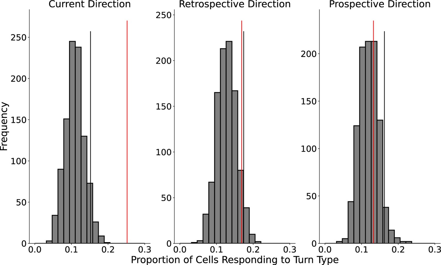
Lack of encoding of retrospective or prospective direction.
A generalized linear model (GLM) approach was used to test for encoding of retrospective or prospective directions within single fields. The following model was fit to each field: Rate+1 ~ DirCurrent+DirProspective+ DirRetrospective+time, where time is represented as a natural spline with 3 df. The model is interpreted as testing the effect on firing rate of individual terms corresponding to previous, current, and next direction as well as time. The glm function from stats in R was used. Post hoc comparison tests between levels of the same factor were performed using emmeans (Lenth, 2022). The proportion of fields with a significant effect of current direction (25.2%) was greater than the 95th percentile of a shuffled distribution created by shuffling the sample firing rates from the sample direction labels. However, the proportions of fields with an effect of retrospective (16.9%) and prospective directions (13.2%) were not greater than the 95th percentiles of their respective shuffled distributions. The effect of retrospective direction trended toward significance (p=0.069).
Figure 4 with 1 supplement
Repeating versus non-repeating fields directionality and spatial decoding.
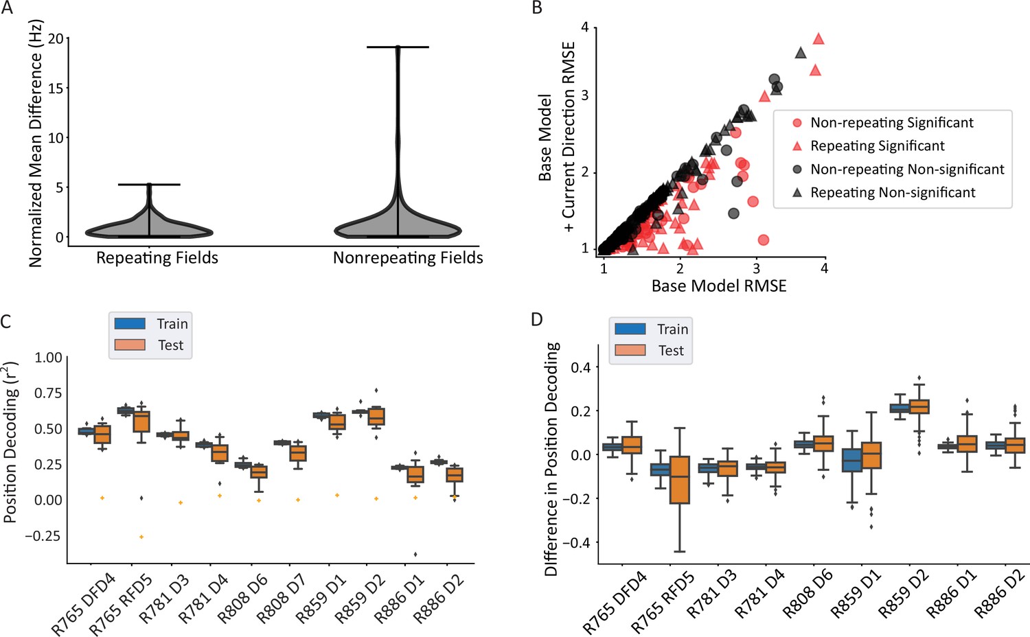
(A) The distribution of directional firing metrics for each repeating or non-repeating field. Directional firing was computed, as above, as the unsigned difference between the average firing rate in each of the two directions through the field. The two populations were not different from one another (repeating fields 0.88±0.81 versus non-repeating fields 1.21±1.97 normalized Hz; Mann-Whitney U=11,883, p=0.49). (B) Generalized linear model (GLM) model comparison as in Figure 3C, separated by whether the field was repeating or not. There was no difference in either the proportion of fields that were significant in each category (69/172 repeating field portions versus 51/125 field portions, χ2(1)=0.001, p=0.97) or the degree of improvement to the model fit (root mean square error [RMSE] differences in base versus direction model, repeating=–0.104, non-repeating=–0.145, Mann-Whitney U=9764, p=0.088). The same outlier was removed from visualization as in Figure 3C. (C) Position decoding from training and testing data across datasets. Each box plot is the decoding performance (from training or test epochs) from 1000 rotations of the training/test window boundaries. Orange dot indicates the 95th percentile of a shuffled distribution formed by circularly shuffling the rat’s position with respect to the neural population activity vector. The median decoder performance was 0.38±0.29 (IQR). (D) The difference in decoder performance from datasets in C using only repeating or non-repeating neurons. (See Figure 4—figure supplement 1 for spatial decoding by repeating or non-repeating cell type.) The group with the smaller sample size was downsampled 10 times per rotation of the train/test windows and the performance averaged. Non-repeating performance was subtracted from repeating performance and the distribution of differences is shown for train and test sets. Most datasets had differences near 0, indicating that overall, there was little difference in decoding performance for repeating versus non-repeating cells.
Figure 4—figure supplement 1

Continuous decoding by repeating type.
The continuous position decoding done in Figure 4 was repeated with either only repeating or only non-repeating neurons to further test whether there was a difference in the position signal afforded from their neural activity. The left column shows the r2 score of the model on the training data, while the right column shows the r2 score of the model on held-out data. For repeating cells alone the average r2 score = 0.11 ± 0.14 while for the non-repeating neurons the average r2=0.11 ± 0.12, suggesting little difference in their ability to provide a spatial signal.
Figure 5 with 2 supplements
Nonconservation of repeating field directionality.
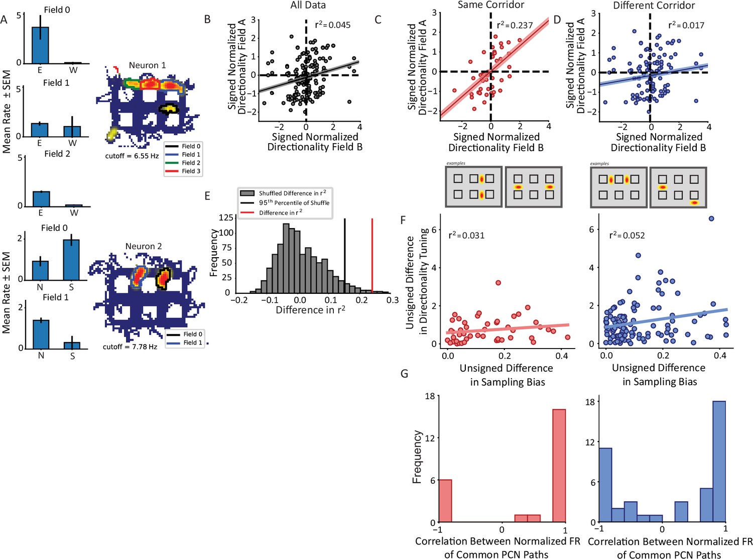
(A) Examples of repeating neurons with directional tuning that was not conserved across fields. Top, neuron with four fields in horizontal alleys, three of which had sufficient sampling for analysis. Fields 0 and 2 preferred east over west while field 1 was untuned. Bottom, two fields primarily in vertical alleys that display opposite tuning patterns such that field 0 fires more strongly for south and field 1 for north. (B) The pairwise correlation in directionality tuning between all pairs of aligned repeating fields within the same cell. The directionality index for each field was normalized by the field’s maximum. The correlation between points explains little of their variance (r2=0.045, p=0.007). Pairs of fields were overall not much more likely to share (i.e. Quadrants I and III) as to not share (i.e. Quadrants II and IV) directional tuning. (C, D) Field pairs were broken down based on whether the fields were on the same corridor or different corridors. Two examples of each type of relationship are shown (bottom schematics). North and east were taken as positive, by convention. Field pairs on the same kind of segment had a higher correlation (r2=0.237, p=0.00012) than those that were on different segments (r2=0.017, p=0.125). The difference between the correlations was significant using a Fischer’s r-to-Z transformation (independent sample, one-sided test, z=2.49, p=0.0063). (E) The difference in panels C–D was corroborated using a shuffling procedure. The labels for field pairs were shuffled while maintaining sample size. The difference r2same_shuffle – r2different_shuffle was computed. The 95th percentile of this distribution was 0.155 which was less than the observed difference of 0.219. (F) The pairwise comparison of sampling bias and directional tuning between fields on same or different corridors. The sampling bias explained little in the pattern of directionality differences between fields in either corridor group. (G) Correlation between average response to each trajectory shared by fields comprising pairs on same (red) or different (blue) corridors showed bimodal distributions. A Hartigan’s test showed that the distributions were not unimodal.
Figure 5—figure supplement 1

Corridor analysis controls.
(A) Distance between centers of mass (COMs) of fields comprising pairs on the same corridor (red) or different corridors (blue). Euclidean distance between field COMs (using straight-line distance between COMs, ignoring track geometry) on the same corridor was slightly shorter (17.55±7.56 bins) than that of those on different corridors (20.1±8.27 bins) (Mann-Whitney U=2097.5, p=0.031). (B) Travel distance between subsequent visits to fields comprising a pair on the same corridor (red) or a different corridor (blue). The unique pairs of alleys were used from each dataset based on all pairs of alleys on which repeating fields were located; i.e., if two simultaneously recorded repeating cells had pairs of fields in the same alleys, that alley pair was used only once. For each alley pair, the average path length was calculated as the number of alleys separating successive visits to each alley of the pair, for all visits to the alleys. Each path length between alleys on different corridors was adjusted by –1 because it was impossible for there to be no intervening alleys for those paths (i.e. fields on alleys on different corridors could not be adjacent). The average path length for the same corridor pairs was shorter (4.17±2.54 alleys) compared to different corridors (8.01±3.47 alleys) (Mann-Whitney U=607, p=8.04 × 10⁻¹¹).
Figure 5—figure supplement 2
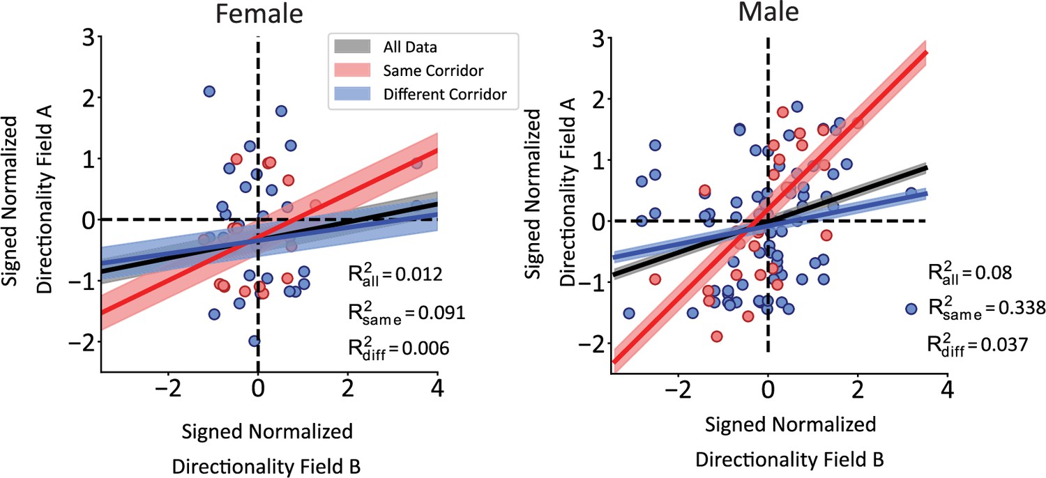
Lack of differences between male and female rats.
Rat sex was approximately balanced with 3 males and 2 females in the dataset. CA1 responses were similar between the sexes in the main analyses presented here. Male and female rats did not have a statistically different number of operationally defined repeating neurons (male 26/97, female 30/82, Pearson’s chi-square test χ2(1)=0.74, p=0.38). CA1 neurons were no more likely to be directionally tuned in male versus female rats (29.1% of male units [58/199] directional, 31.5% [35/111] of females, Pearson’s chi-square test χ2(1)=0.039, p=0.84). Last, the figure panels show the results of the same corridor versus different corridor analysis. Although the results were qualitatively similar between the sex groups, quantitative differences may be due to differences in sample size, and we do not place much confidence in this result based on data collected from only 2 female and 3 male rats.
Figure 6 with 2 supplements

Temporal dynamics.
(A) Examples of neurons with temporally dynamic place fields. Top, neuron with single field in a vertical alley. The field rate increases to a peak that is maintained for roughly 10 min, before slowly decaying toward near silence over the rest of the session. Middle, repeating neuron with two fields in vertical alleys. The fields appear to have complex periodic dynamics over time. Further, they appear to be in an approximate antiphase relationship in approximately the first half of the session, such that when the west field (black) is more active, the east field (blue) is at a local trough and vice versa. Bottom, repeating cell with four fields, three of which are in horizontal alleys. Each field peaks with a different delay and then gradually decays over time. The delays are such that the times during which each field is active tile the whole session and the cell maintains its overall activity over time. (B) A generalized linear model (GLM) likelihood ratio test to determine whether fields are temporally dynamic. The base model included current direction, for an analogous reason as to why time was included in the base model when testing for current direction. Time was represented as a natural spline with three degrees of freedom. A significant number of fields changed their firing rates over time (83/296 field pieces, p=2.07 × 10–38, alpha = 0.0083 for three spline knots multiplied by (up to) two orientations per field). (C) Pairwise comparisons of the firing rate time series of pairs of repeating fields were computed using Pearson’s correlation. The firing rate time series were interpolated to equate their sample sizes using a piecewise cubic Hermite interpolating polynomial (PCHIP) interpolation. The distribution was centered near zero with a wide distribution (mean = 0.049 ± 0.26). (D) Pairwise correlations between activity patterns in different time windows. Time windows closer together are more correlated than those further away. There was no significant difference in the slope of the decorrelation between repeating and non-repeating neurons (Figure 6—figure supplement 1). (E) Example time window from single dataset showing portion of data held out for training (white space, center) and the decoding performance on the rest of the data divided into temporal windows. Shaded region is shuffle. Red corresponds to x position data, green to y position data. (F) Distribution of Spearman correlation of decoding performance before or after the training window shows the gradual decrease in decoder performance with increasing distance from the training window.
Figure 6—figure supplement 1

Temporal drift in repeating versus non-repeating neurons.
Population vector correlations as in Figure 6D but done separately for repeating and non-repeating fields. Linear regression model for repeating neurons: r2=0.20, slope = –0.067, p=9.8 × 10⁻⁸. Linear regression model for non-repeating neurons: r2=0.16, slope = –0.053, p=4.01 × 10⁻¹².
Figure 6—figure supplement 2

Shuffling test of temporal dynamics.
To corroborate the generalized linear model (GLM) results related to temporal dynamics in Figure 6B, a shuffling test was employed. For each field, the passes through the field were labeled with which third of the session they occurred. Then, for each of 1000 iterations, these labels were permuted for each field. Then, the GLM procedure was repeated as in Figure 6B. The proportion of fields with a (spurious) demonstration of time dynamics was a single data point in this null distribution. Left, in black, is the null distribution which is significantly lower than the real proportion (red line).
Additional files
-
Supplementary file 1
Alley traversals on which the animal was rewarded were excluded from all main text analyses as any CA1 response to the reward itself was an undesirable source of variability.
However, major analyses were re-run with rewards included (i.e. all passes through the alley) to test whether this changed the results. In each of three major analyses, the inclusion of reward trials did not qualitatively change the results compared to when these trials were excluded. It should be noted for the re-analysis of Figure 3B, the numerator decreased by a large amount despite little change to the overall pool of fields tested. The fact that including rewards did not result in many more fields being included can be explained by the fact that rewards were uniformly distributed across the track so their removal decreased the samples from all fields evenly, resulting in little change to the number of fields included for analysis. The fact that the numerator (i.e. directional fields) decreased could be explained by the fact that rewarded trials introduced variability; indeed this was the justification for their removal, and this variability might have reduced the statistical power of the Mann-Whitney test from Figure 3C.
- https://cdn.elifesciences.org/articles/85599/elife-85599-supp1-v1.docx
-
MDAR checklist
- https://cdn.elifesciences.org/articles/85599/elife-85599-mdarchecklist1-v1.docx
Download links
A two-part list of links to download the article, or parts of the article, in various formats.
Downloads (link to download the article as PDF)
Open citations (links to open the citations from this article in various online reference manager services)
Cite this article (links to download the citations from this article in formats compatible with various reference manager tools)
Leveraging place field repetition to understand positional versus nonpositional inputs to hippocampal field CA1
eLife 14:e85599.
https://doi.org/10.7554/eLife.85599


