Figures and data in Barcode-free multiplex plasmid sequencing using Bayesian analysis and nanopore sequencing

Figures
Tables
Additional files

6 figures, 2 tables and 2 additional files

Figures

Figure 1

Download asset Open asset

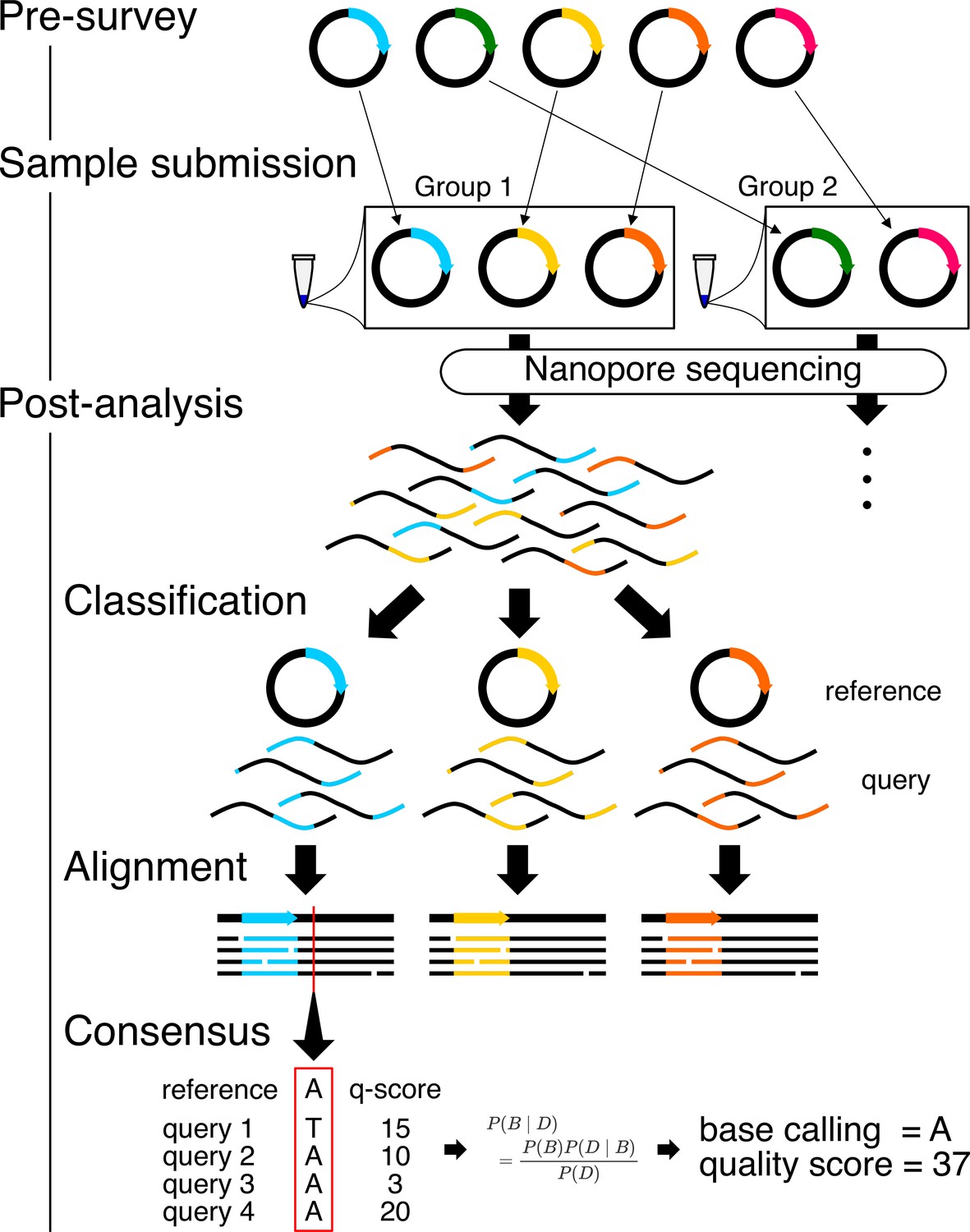
Workflow for Simple Algorithm for Very Efficient Multiplexing of Oxford Nanopore Experiments for You (SAVEMONEY).

The algorithm consists of three steps: pre-survey, sample submission, and post-analysis. The pre-survey step identifies the optimal combination of plasmids that will permit suitable accuracy for the classification step of the post-analysis. Plasmids with divergent sequences are grouped together, and those with very similar sequences are classified into different groups. After sample submission and sequencing, the post-analysis component, which consists of three different steps, is performed to deconvolve the obtained results. Reads (query sequences) are first classified based on their similarity to the plasmid blueprint/map (reference sequence). Reads are then aligned against reference sequences. Finally, consensus sequences and quality scores are calculated based on base calls, quality scores from each read, and the reference sequence, using Bayesian analysis.

Figure 2

Download asset Open asset

Examples of the pre-survey outputs.

Sequences of 14 different plasmids were analyzed with the indicated $d i s t a n c e_t h r e s h o l d$ and $n u m b e r_o f_g r o u p s$ values. Levenshtein distance between each plasmid pair is displayed in heatmaps, which were subsequently used to generate the dendrograms displayed on the right side of the heatmap. The dotted red lines in the dendrogram represent the $d i s t a n c e_t h r e s h o l d$ values, enabling visualization of the results of clustering, i.e., plasmids with distances less than the red lines were classified in the same cluster. Based on this clustering results of similar plasmids, plasmids were classified into groups for sequencing submission, with groups displayed in red and blue (a), red, blue, and magenta (b), or red, blue, magenta, and cyan (c). Levenshtein distance between each plasmid is also emphasized by the colored frames within each group, and plasmids classified into the same cluster are grouped in different groups. Note that P1–P14 here are different from example plasmids used in Figures 3 and 4.

Figure 2—source data 1 Results of pre-survey used to make Figure 2a.: https://cdn.elifesciences.org/articles/88794/elife-88794-fig2-data1-v1.txt
Download elife-88794-fig2-data1-v1.txt
Figure 2—source data 2 Results of pre-survey used to make Figure 2b.: https://cdn.elifesciences.org/articles/88794/elife-88794-fig2-data2-v1.txt
Download elife-88794-fig2-data2-v1.txt
Figure 2—source data 3 Results of pre-survey used to make Figure 2c.: https://cdn.elifesciences.org/articles/88794/elife-88794-fig2-data3-v1.txt
Download elife-88794-fig2-data3-v1.txt

Figure 3

Download asset Open asset

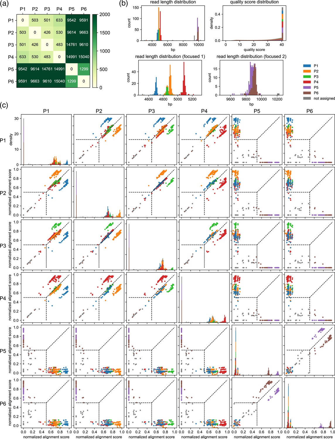
Example results after the classification step for a set of six moderately related plasmids.

(a) Results of the pre-survey against plasmid sets used in (b, c). (b) Read length and the quality score distributions. (c) Scatter plots of normalized alignment scores. Normalized alignment scores were calculated for each read over all reference plasmids and displayed as scatter plots. Density plots of the normalized alignment scores are also displayed for each reference plasmid in the diagonal panel, which is the projection of each scatter plots against horizontal axes. The y-axis ranges of these diagonal panels are shared. The vertical and the horizontal positions of dashed lines correspond to $s c o r e_t h r e s h o l d$ value. These data depict results of classification performed with a $s c o r e_t h r e s h o l d$ value of 0.5. Note that P1–P6 here are different from example plasmids used in Figures 2 and 4.

Figure 3—source data 1 Fastq file containing original data used to make Figure 3b and c.: https://cdn.elifesciences.org/articles/88794/elife-88794-fig3-data1-v1.zip
Download elife-88794-fig3-data1-v1.zip
Figure 3—source data 2 Csv file containing raw data used to make Figure 3b.: https://cdn.elifesciences.org/articles/88794/elife-88794-fig3-data2-v1.csv
Download elife-88794-fig3-data2-v1.csv
Figure 3—source data 3 Csv file containing raw data used to make Figure 3c.: https://cdn.elifesciences.org/articles/88794/elife-88794-fig3-data3-v1.csv
Download elife-88794-fig3-data3-v1.csv

Figure 4

Download asset Open asset

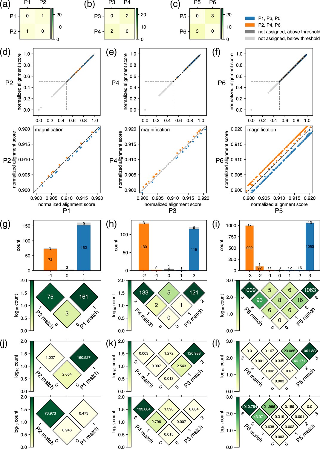
Example results after the classification step for closely related plasmids.

(**a–c**) Results of the pre-survey against plasmid sets. (**d–f**) Scatter plots of normalized alignment scores for the plasmid pairs. The vertical and the horizontal positions of dashed lines correspond to $s c o r e_t h r e s h o l d$ values. These data depict results of classification performed with a $s c o r e_t h r e s h o l d$ value of 0.5. (**g–i**) Breakdowns of reads covering the regions where the plasmids differ in sequence. In the rotated heatmap at the bottom of (g), the axis labeled as ‘P1 match’ represents the number of bases matching the P1 sequence in the regions where the sequences of P1 and P2 differ, whereas the axis labeled as ‘P2 match’ represents the equivalent for P2. The values in each cell represent the number of observed reads matching the values of the two axes at that position. The subtraction of ‘P1 match’ from ‘P2 match’ is represented by the horizontal axis, which is also shared with the x-axis of the histogram on top, where the sum projection of the heatmap is displayed. In the histogram, the breakdown of classification is represented by color: blue for reads classified to P1, orange for reads classified to P2, gray for unclassified reads with a score above $s c o r e_t h r e s h o l d$ , and light gray for unclassified reads with a score below $s c o r e_t h r e s h o l d$ . Because the normalized alignment scores for the two plasmids are the same where the value on the horizontal axis is 0, reads are not classified to either plasmid; therefore, the middle bar of the histogram is colored with either gray or light gray. The same interpretation applies to (h) and (i). (**j–l**) Summary of the fitting results. Based on the estimated parameters displayed in Table 1, the rotated heatmaps representing the breakdowns of reads originating from P1, P3, and P5 (upper panels) and P2, P4, and P6 (lower panels) were generated. Note that P1–P6 here are different from example plasmids used in Figures 2 and 3.

Figure 4—source data 1 Fastq file containing original data used to make Figure 4d and g.: https://cdn.elifesciences.org/articles/88794/elife-88794-fig4-data1-v1.zip
Download elife-88794-fig4-data1-v1.zip
Figure 4—source data 2 Fastq file containing original data used to make Figure 4e and h.: https://cdn.elifesciences.org/articles/88794/elife-88794-fig4-data2-v1.zip
Download elife-88794-fig4-data2-v1.zip
Figure 4—source data 3 Fastq file containing original data used to make Figure 4f and i.: https://cdn.elifesciences.org/articles/88794/elife-88794-fig4-data3-v1.zip
Download elife-88794-fig4-data3-v1.zip
Figure 4—source data 4 Csv file containing raw data used to make Figure 4d and g.: https://cdn.elifesciences.org/articles/88794/elife-88794-fig4-data4-v1.csv
Download elife-88794-fig4-data4-v1.csv
Figure 4—source data 5 Csv file containing raw data used to make Figure 4e and h.: https://cdn.elifesciences.org/articles/88794/elife-88794-fig4-data5-v1.csv
Download elife-88794-fig4-data5-v1.csv
Figure 4—source data 6 Csv file containing raw data used to make Figure 4f and i.: https://cdn.elifesciences.org/articles/88794/elife-88794-fig4-data6-v1.csv
Download elife-88794-fig4-data6-v1.csv

Figure 5

Download asset Open asset

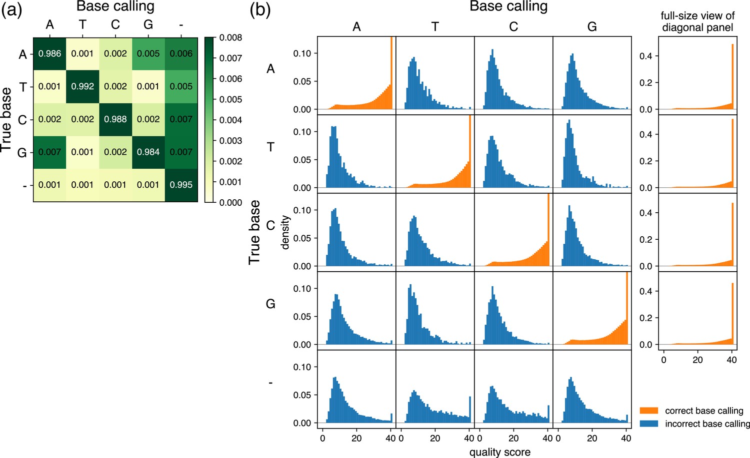
Characteristics of base calling used for prior information.

(a) Grid showing error ratios for each base calling event. Based on the results obtained from samples analyzed by R10.4.1 flow cells with V14 library preparation chemistry by Oxford Nanopore Technologies via the Plasmidsaurus service, the frequency was analyzed for base calling of each pore (column labels) and the results of the consensus sequence (row labels) at each position. In the context of base calling, ‘–’ represents bases that were base-called in the consensus sequence but skipped in the reads from each pore. In the context of consensus sequencing, ‘–’ represents bases that do not appear in the consensus sequence but were base-called from pores. The color of the diagonal panels is saturated because of the contrast range focusing on subtle differences of the non-diagonal panels. Of note, the sum of the rows is 1, but the sum of the displayed numbers may be slightly different from 1 because the fourth decimal place is rounded in the grid. (b) Quality score distributions for each base calling event. The base calling of each pore (column labels) and the results of the consensus sequence (row labels) at each position were classified, and probability density plots and quality scores were calculated and displayed. The y-axis is shared by all panels and is scaled to focus on panels in which the true base and base calling are not the same (incorrect base calling, blue). Therefore, the density of maximum quality score is out of the range of the display area in the diagonal panels (correct base calling, orange), and full-size plots are provided to the right. Note that there are no density plots when base calling was skipped in the reads from each pore (column corresponding to the label ‘–’ in (a)).

Figure 5—source data 1 Text file containing raw data used to make Figure 5.: https://cdn.elifesciences.org/articles/88794/elife-88794-fig5-data1-v1.txt
Download elife-88794-fig5-data1-v1.txt

Figure 6

Download asset Open asset

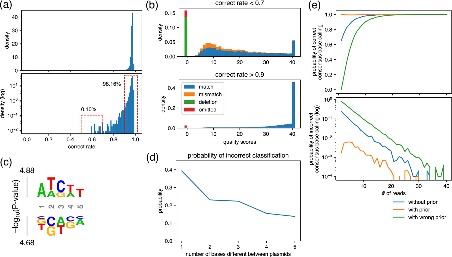
Analysis for the maximum similarity between plasmids that can be mixed and the minimum number of required reads.

(a) Density plot of the rate of reads with correct base calling. The rate was calculated at each position of plasmids and displayed using representative nanopore sequencing results. (b) Averaged quality score distribution of reads with correct rate of less than 0.7 (upper panel) and more than 0.9 (bottom panel). The corresponding regions are displayed with dashed red frames in (a). Of note, ‘omitted’ represents reads that did not cover the focused position. (c) Probability logo plot. Statistical significance (−log₁₀[p-value]) was calculated for a 5-mer around the positions that showed correct rate lower than 0.7 in (a) using those that showed more than 0.9 as a background. Enriched residues are stacked on the top, whereas depleted residues are stacked on the bottom. (d) Estimated probability of incorrect classification. Based on the match/mismatch/deletion ratio of reads obtained in the ‘worst-case scenario’, i.e., top panel in (b), the probability of incorrect classification of a read was calculated assuming that two plasmids that differ by the indicated base(s) were mixed. (e) Estimated probability of correct/incorrect consensus base calling. Based on the quality score distribution obtained in the ‘worst-case scenario’, i.e., top panel in (b), the indicated number of reads were generated in silico, and the consensus base calling was calculated using Simple Algorithm for Very Efficient Multiplexing of Oxford Nanopore Experiments for You (SAVEMONEY). The simulation was performed 10,000 times for each condition to calculate the probability of correct/incorrect consensus base calling.

Figure 6—source code 1 Source code used to make Figure 6d.: https://cdn.elifesciences.org/articles/88794/elife-88794-fig6-code1-v1.zip
Download elife-88794-fig6-code1-v1.zip
Figure 6—source code 2 Source code used to make Figure 6e.: https://cdn.elifesciences.org/articles/88794/elife-88794-fig6-code2-v1.zip
Download elife-88794-fig6-code2-v1.zip
Figure 6—source data 1 Csv file containing raw data used to make Figure 6a.: https://cdn.elifesciences.org/articles/88794/elife-88794-fig6-data1-v1.csv
Download elife-88794-fig6-data1-v1.csv
Figure 6—source data 2 Csv file containing raw data used to make Figure 6b.: https://cdn.elifesciences.org/articles/88794/elife-88794-fig6-data2-v1.csv
Download elife-88794-fig6-data2-v1.csv
Figure 6—source data 3 Text file containing raw data used to make Figure 6c.: https://cdn.elifesciences.org/articles/88794/elife-88794-fig6-data3-v1.txt
Download elife-88794-fig6-data3-v1.txt
Figure 6—source data 4 Csv file containing raw data used to make Figure 6e.: https://cdn.elifesciences.org/articles/88794/elife-88794-fig6-data4-v1.csv
Download elife-88794-fig6-data4-v1.csv

Tables

Table 1

The fitting results summarized in Figure 4j–l.

The values for the fitted parameters are displayed in ‘Error rate’ and ‘Total reads’ columns. The rotated heatmaps in Figure 4j–l were generated based on these estimated parameters. For P1, P3, and P5, the sum of values in heatmap cells whose location on the horizontal axis are above 0, below 0, and 0 are shown as ‘Correctly classified reads’, ‘Wrongly classified reads’, and ‘Reads not classified’ columns, respectively. For P2, P4, and P6, below 0, above 0, and 0 are shown as ‘Correctly classified reads’, ‘Wrongly classified reads’, and ‘Reads not classified’ columns, respectively. Finally, the values in ‘Rate of incorrect classification’ columns for each plasmid were calculated by dividing the values of ‘Wrongly classified reads’ for the other plasmids in the same set by the total number of reads estimated to be classified to the focusing plasmid, which is different from values displayed in the ‘Total reads’ column. Specific equations are provided in the footnote to the table.

		Error rate	Total reads	Correctly classified reads	Wrongly classified reads	Reads not classified	Rate of incorrect classification
Set 1	P1	0.0188	163.607	160.527^a1	1.027^b1	2.054	0.002939^c1
Set 1	P2	0.0188	75.393	73.973^a2	0.473^b2	0.946	0.013691^c2
Set 2	P3	0.0155	124.826	123.531^a3	0.010^b3	1.285	0.000089^c3
Set 2	P4	0.0155	137.223	136.000^a4	0.011^b4	1.413	0.000074^c4
Set 3	P5	0.0213	1131.757	1131.249^a5	0.170^b5	0.338	0.000143^c5
Set 3	P6	0.0213	1077.833	1077.349^a6	0.162^b6	0.322	0.000158^c6

c1=b2/(a1+b2); c2=b1/(a2+b1); c3=b4/(a3+b4); c4=b3/(a4+b3); c5=b6/(a5+b6); c6=b5/(a6+b5).

Key resources table

Reagent type (species) or resource	Designation	Source or reference	Additional information
Recombinant DNA reagent	pCDH1-lyn10-mCherry-LOVPLD* (plasmid)	This paper	P1 in Figure 2; Plasmid used in PMID:38559292 with silent mutation
Recombinant DNA reagent	pCDH1-lyn10-mCherry-LOVPLD (plasmid)	PMID:38559292	P2 in Figure 2
Recombinant DNA reagent	pCDH1-lyn10-mCherry-LOVPLD** (plasmid)	This paper	P3 in Figure 2; Plasmid used in PMID:38559292 with silent mutation
Recombinant DNA reagent	pCDH1-lyn10-mCherry-LOVPLD*** (plasmid)	This paper	P4 in Figure 2; Plasmid used in PMID:38559292 with silent mutation
Recombinant DNA reagent	pET-17b-mod2_6xHis-PLDs48-HiBiT (plasmid)	This paper	P5 in Figure 2
Recombinant DNA reagent	pET-17b-mod2_6xHis-PLD-HiBiT (plasmid)	This paper	P6 in Figure 2
Recombinant DNA reagent	pET-17b-mod2_6xHis-PLDs4-HiBiT (plasmid)	This paper	P7 in Figure 2
Recombinant DNA reagent	pET-17b-mod_6xHis-PLDs48**-HiBiT (plasmid)	This paper	P8 in Figure 2
Recombinant DNA reagent	pET-17b-mod_6xHis-PLDs48*-HiBiT (plasmid)	This paper	P9 in Figure 2
Recombinant DNA reagent	pET-17b-mod_6xHis-PLDs48-HiBiT (plasmid)	This paper	P10 in Figure 2
Recombinant DNA reagent	pET-17b-mod_6xHis-PLDs27L484F-HiBiT (plasmid)	This paper	P11 in Figure 2
Recombinant DNA reagent	pET-17b-mod_6xHis-PLD-HiBiT (plasmid)	This paper	P12 in Figure 2
Recombinant DNA reagent	pET-17b-mod_6xHis-PLDs4A326T-HiBiT (plasmid)	This paper	P13 in Figure 2, P1 in Figure 3
Recombinant DNA reagent	pET-17b-mod_6xHis-PLDs4-HiBiT (plasmid)	This paper	P14 in Figure 2, P2 in Figure 3
Recombinant DNA reagent	pmNeonGreen-N1 (plasmid)	Other	P1 in Figure 3; a gift from the Lammerding Laboratory, Cornell University, Ithaca, NY, USA
Recombinant DNA reagent	mCherry-Spo20 (plasmid)	Other	P2 in Figure 3; a gift from the Frohman Laboratory, Stony Brook University, Stony Brook, NY, USA
Recombinant DNA reagent	GFP-PASS (plasmid)	Other	P3 in Figure 3; a gift from the Du Laboratory, The University of Texas Health Science Center at Houston, Houston, TX, USA
Recombinant DNA reagent	iRFP-PASS (plasmid)	PMID:31999306	P4 in Figure 3
Recombinant DNA reagent	pcDNA3_P18-CIBN-P2A-CRY2-mCherry-PLD(1-17) (plasmid)	PMID:37217787	P5 in Figure 3
Recombinant DNA reagent	pcDNA3_CRY2-mCherry-PLD(2-27)-P2A-CIBN-CAAX (plasmid)	PMID:37217787	P6 in Figure 3
Recombinant DNA reagent	PLD-mCherry-Rab7 (plasmid)	Other	P3 in Figure 3; constructed by Reika Tei (Baskin Lab)
Recombinant DNA reagent	dPLD-mCherry-Rab7 (plasmid)	Other	P4 in Figure 3; constructed by Reika Tei (Baskin Lab)
Recombinant DNA reagent	pGFPN1-PL5(143–271)-EGFP-S161D	PMID:39209962	P5 in Figure 3
Recombinant DNA reagent	pGFPN1-PL5(143–271)-EGFP	PMID:35952650	P6 in Figure 3
Software, algorithm	SAVEMONEY	This paper	version 0.3.4