Neural correlates of perceptual similarity masking in primate V1
Figures

Target-background similarity masking and behavioral task.
(A) Low contrast orientated targets can be easily detected on uniform background. (B) Similarity masking is induced by an orientated background. The same additive target from (A) becomes hard to detect when target orientation matches background orientation (see also perceptual demonstration in Supplementary file 1). (C–E) Orientation masking was assessed in two awake behaving macaque monkeys performing a target detection task. Monkey commence the task by fixating at the small bright square (C). A few moments later, a 4° raise-cosine-masked background grating was flashed at ~3° eccentricity for target detection (D). The horizontal white bar represents one degree of visual angle. In 50% of the trials, a small additive horizontal Gabor target was also added to the background (E). The monkey indicated the presence of the target by making a saccade to the target location, and indicated target absent by maintaining gaze at the fixation point. The Gabor target was always the same – a cosine centered, horizontal Gabor at 4cpd on 0.33° FWHM envelope. The background grating was also cosine-centered at 4cpd such that the background completely aligned with the target when they were the same orientation (as in B). Orientation of the grating ranged from 0° to 90° with respect to the Gabor target and was randomized between trials. Bg – background; TBg – target plus background.
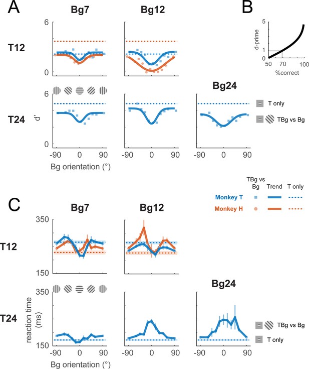
Behavioral effect of target-background similarity masking.
(A) Target detection performance in monkeys was affected by the orientation of the background grating over a variety of target contrast (T## = ##% contrast target) and background contrast levels (Bg## = ##% contrast background). Signal detection measure d-prime (d’) of the target is plotted for uniform background (dotted lines), and for each background orientation (markers). In most cases, there was a general performance reduction from uniform background to a grating background. Additionally, performance was further reduced when the background orientation was more aligned to the target (0°). A fitted Gaussian (solid line) illustrates the performance change due to orientation masking. d’ was calculated from the hit rate (correctly reporting target present) and the false alarm rate (reporting target present when it was absent). The relationship between d’ and optimum performance level in percent correct is plotted in (B). (C) Reaction time – calculated from stimulus onset to saccade initiation for Hit trials – is plotted for uniform background (dotted lines) and for each background orientation (solid lines). Error bars indicate the standard error of the mean. Data were pooled within each monkey across experiments. Each experiment contains a single combination of target and background contrast levels, with uniform background and orientated background trials assessed in separate blocks.
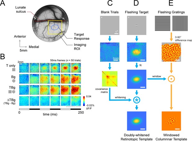
VSD response and decoder schematic.
(A) A cranial chamber and a transparent artificial dura provided chronic imaging access to V1 of the monkey. V2 is completely hidden in the lunate sulcus based on the retinotopic map taken in a separate imaging session (Figure 3—figure supplement 1). Imaging ROI and target response at 2 SD of the fitted Gaussian from the example recording in B-E are illustrated. (B) Example recording of the voltage-sensitive dye (VSD) response in an 8x8 mm imaging region-of-interest (ROI). Response to the Gabor target on uniform background could be easily identified in VSD (top row). The visual span of the background grating extended beyond the coverage of the imaging window, evoking an encompassing response over the entire ROI (2nd row). When the background was presented with the additive target, the response to the target was diminished (3rd and 4th rows). Each VSD response map were averaged across 50 trials, over 5 frames captured at 100 Hz. T only – target only; Bg – background only; TBg – target and background; ΔTBg – target and background minus background only. (C) Target response was extracted at the retinotopic scale by estimating its response profile with a two-dimensional Gaussian. The profile was estimated from response from a separate recording block on each experiment day. To optimized signal-to-noise, in this recording block, the target was flashed repeatedly at 5 Hz while the monkey maintained fixation. The effect of spatially correlated VSD noise was minimized by estimating a whitening kernel from trials without stimulus presentation (see Methods). (D) Target response was extracted at the columnar scale by estimating the orientation map within the imaging area. This was constructed from full-field gratings flashed at 5 Hz in a separate recording block on each experiment day (see Methods). The columnar map in the 0°–90° axis was extracted and windowed down to the retinotopic profile to identify the columnar scale response of the target.
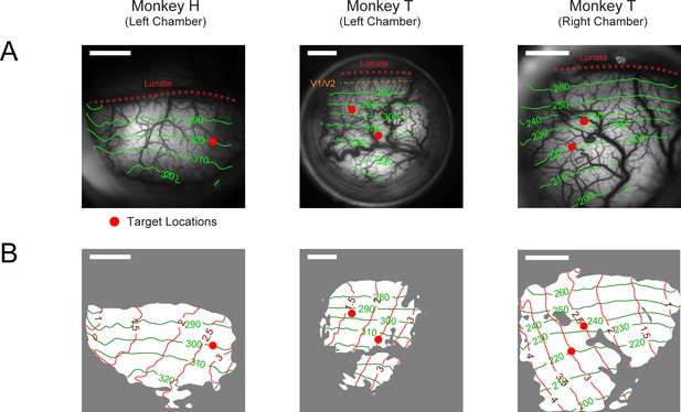
Retinotopy of imaging chambers and target placement positions.
A separate VSD imaging experiment was conducted for each chamber with special retinotopic scanning stimuli (see Methods). (A) Photograph of the imaging chamber overlaid with contour lines (green) of polar angles relative to the horizontal meridian of the visual field. Angular values were anti-clockwise from the right horizontal meridian. The V1-V2 border (dashed orange line) is at 270°. This border is hard to estimate and is believed to be 0.7 mm from the lunate in Monkey T’s left visual cortex chamber (col 2). For the other two chambers, the V1-V2 border is estimated to be inside the lunate sulcus (dashed red line). (B) The same imaging areas as in A marked with both the angular (green) and eccentricity (red) contour lines. Area with good VSD staining on the day of retinotopy is marked in white. Red dots in A and B indicate where the target was placed. The position of the target in cols 2–3 was moved between experiments to optimize for the imaging outcome as a response to the quality of VSD staining of the day. Scale bars indicate 4 mm in length.

Retinotopic template dynamics and correlation to behavior.
(A–F) Average response and dynamics from recordings with 12% target contrast (T12) and 7% background contrast (Bg7). (A) Response time course from stimulus onset (t=0ms) for background only trials. Background orientation are identified by color. Backgrounds with the same clockwise and anticlockwise orientation disparity from the target were pooled. (B) Response time course with the same additive target on different oriented background. Response of the target on uniform gray background is illustrated in black. (C) The target-evoked response time course was obtained by subtracting background only response (A) from response to target & background (B). Target evoked response was initially strongest for backgrounds close to 0° (red), then inverted around t=100ms such that response became the stronger for background closer to 90° (blue). (D) Response was averaged over 50–200ms and fitted with a Gaussian (gray) to illustrate the change in response magnitude with respect to background orientation. The neural-behavioral correlation of the response against behavioral response (F) is printed with p significance value. Here, response to clockwise and anti-clockwise background orientations are plotted separately. Size of markers indicate the number of trials tested for each orientation. Black line indicates the response of the target only trials integrated over the same window. (E) The animals’ behavior performance was anti-correlated with the initial phase of the retinotopic response, and was more aligned in the latter phase. Correlation coefficient was calculated across background orientations between each frame of the retinotopic response in (C) against the overall behavior performance in (F). Red dots indicate frames reaching statistical significance (p<0.05, t-test for correlation coefficient, see Methods). The neural-behavioral correlation crosses from negative to positive at t=130ms. (F) Behavior performance in d’ was calculated as described in Figure 2. Size of markers indicate the number of trials tested for each orientation. Data was pooled across 8 experiments from both monkeys (see Table 1). (G–L) Same as (A–F) for recordings with 24% target contrast (T24) and 12% background contrast (Bg12). Similar trends were observed. The neural-behavioral correlation crosses from negative to positive at t=96ms in (K).
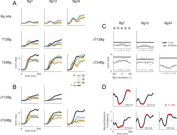
Retinotopic template dynamics and correlation to behavior for all combinations of background and target contrast levels.
Retinotopic response time course using doubly-whitened retinotopic decoding template illustrated in Figure 3. (A) Response time course from stimulus onset (t=0ms), grouped by different combinations of target and background contrast levels. Background orientation is indicated by color. Backgrounds with the same clockwise and anticlockwise orientation disparity from the target were pooled. Response of the target on uniform gray background is illustrated in black. (B) The target-evoked response time course was obtained by subtracting the background only response (A, top row) from the background-plus-target response (rest of A) from the same experiments. (C) Response was averaged over 50–200ms and fitted with a Gaussian (gray) to illustrate the change in response magnitude with respect to background orientation. Neural-behavioral correlation of the integrated response against the behavior performance (Figure 2A pooled across monkeys) are printed with p significance values. Here, response to clockwise and anti-clockwise background orientations are plotted separately. Size of markers indicate the number of trials tested for each orientation. Black line indicates the response of the target only trials integrated over the same window. (D) Correlation coefficient was calculated across background orientations between each frame of the retinotopic response in (B) against the overall behavioral performance for each combination of background and target contrast (Figure 2A pooled across monkeys). Red dots indicate frames reaching statistical significance (p<0.05, t-test for correlation coefficient, see Methods). Data was pooled across experiments from both monkeys (see Table 1).
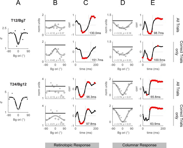
Retinotopic and columnar integrated response and correlation to behavior: correct trials vs all trials.
Response dynamics calculated over all trials as shown in Figure 4 and Figure 5 are replotted in odd rows for comparison against the same stimulus conditions using only correct trials (hits and correct rejections only, even rows). (A) Behavioral performance replotted from Figure 4F and L. Behavioral performance was calculated using all trials (correct and incorrect), and was used for the calculation of correlations when the template response included all trials or just the correct trials. (B, D) Integrated response over 50–200ms from stimulus onset in the same format as Figure 4D. (C, E) Behavioral correlations in the same format as Figure 4E. The vertical lines mark the time of the cross-over from negative to positive correlations (the vertical lines are labeled with the time in ms).
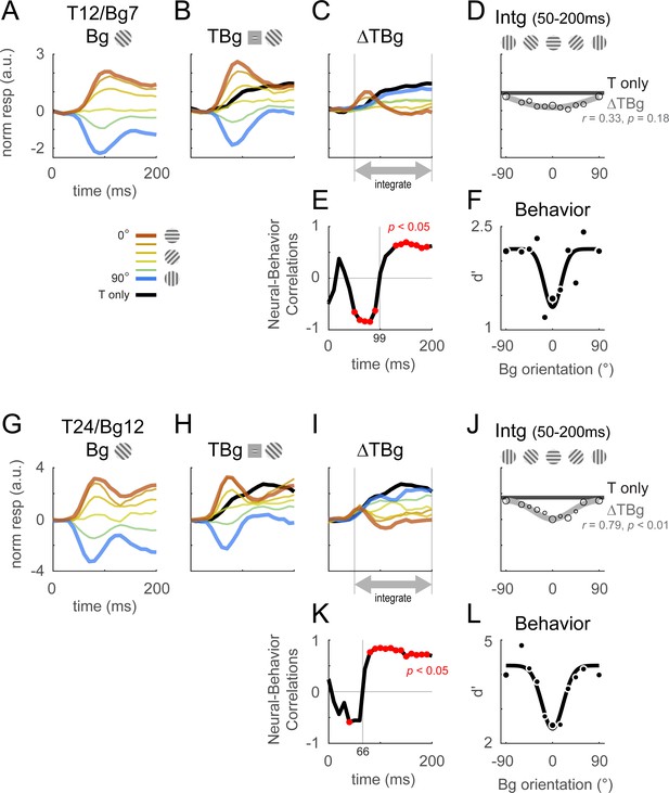
Columnar template dynamics and correlation to behavior.
Same format as Figure 4 with the response examined at the columnar scale. The biphasic response time course observed in the retinotopic scale was more pronounced at the columnar scale. (A–F) Averaged response and dynamics from recordings with 12% target contrast (T12) and 7% background contrast (Bg7). (G–L) Averaged response and dynamics from recordings with 24% target contrast (T24) and 12% background contrast (Bg12). Here, positive response represents relatively stronger activation of the neurons tuned to the target orientation (0°), and negative response represent stronger activation for neurons tuned to the orthogonal orientation (90°). Data pooling and counts are the same as reported in Figure 4. Behavioral correlation crosses from negative to positive at t=99ms in (E), and t=66ms in (K).
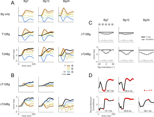
Columnar template dynamics and correlation to behavior for all combinatory background and target contrast levels.
(A–D) Same format as Figure 4—figure supplement 1 with the averaged response examined at the columnar scale. The columnar template extracts the relative strength between neural activity aligned and orthogonal to the target orientation. Positive response represents relatively stronger activation of the neurons tuned to the target orientation (0°), and negative response represent stronger activation for neurons tuned to the orthogonal orientation (90°). Data pooling and counts are the same as reported in Figure 4—figure supplement 1.

Columnar orientation estimation by populations tuning.
(A) The orientation map obtained for each experiment as described in Figure 3 was windowed to the retinotopic profile of the target. (B) Each pixel was assigned to one of 12 equally spaced orientation selective cluster maps by its preferred orientation. (C) The orientation selective decomposition of VSD response. To a grating stimulus oriented at 0°, the population tuning curve peaks at 0° (solid curve); likewise, the population peak would shift to 45° for a 45° grating (dotted curve). Note that this population response only represents the relative difference in preferred orientation (balanced positive and negative values); the overall neural response offset (retinotopic response) is not captured by this approach. (D) Example of a full population response time course from stimulus onset (t=0ms). (E) Population response can be summed to a complex vector representing the overall population tuning orientation and magnitude.

Dynamics of orientation population response.
(A) Population tuning time course for trials with 12% contrast targets (T12) and 7% contrast backgrounds (Bg7). Averaged response time courses are presented as a heatmap with the y-axis representing the preferred orientation (from Figure 6A–C) and the x-axis time (see key on bottom right) to illustrate the change in the tuning over time. Row 1: Heatmaps for background only trials exhibit clear population tuning in the orientation of the background grating (red horizontal line). Row 2: Heatmaps for background with additive target showing population response dominated by the background orientation rather than the target orientation (0°). Row 3: The target evoked response is obtained by subtracting the background only response Row 1 from the target & background response in Row 2. Masking of the target evoked response was strong for backgrounds oriented near the target orientation (0°). With the background orthogonal to the target, population tuning in the target orientation can be identified. White line identifies the orientation of the population vector (peak tuning) wherever the normalized amplitude of the vector average was great than 0.2 (see Methods). Depending on background orientation, peak tuning appears to be offset from the orientation of the target (e.g. at Bg –45°). Row 4: Heatmap for the target only trials demonstrated clear population tuning in the target orientation (0°, green horizontal line). (B–E) Averaged response in (A) represented as a population vector form and illustrated as a continuous trajectory for each background orientation (color coded). (B) Population tuning trajectory for background only trials. The trajectories commenced in the center of the circle (white dot) and adhered closely to the orientation of the background. Dot on each trajectory indicates the position of the population tuning vector at 100ms. (C) Population tuning trajectory for background with additive target illustrating the biphasic response of this combined stimulus. In the early phase, the heading of the trajectory was a mixture of the background and target (0°) orientations, dominated more by the background. In the late phase, the trajectory made a sharp turn (t≈100ms) such that trajectories appeared to head towards a convergent point on the positive x-axis. (D) The trajectory for the target evoked response, calculated by subtracting the background only response (B) from the corresponding background & target (C). The target evoked response was weak and noisy, but was heading in the general direction of the target orientation (0°). (E) The population tuning trajectory for the target only trials illustrating clear tuning in the target orientation (0°). (F–J) Same as (A–E) for trials with 24% contrast targets (T24) and 12% contrast backgrounds (Bg12). Data was pooled and averaged across both monkeys.
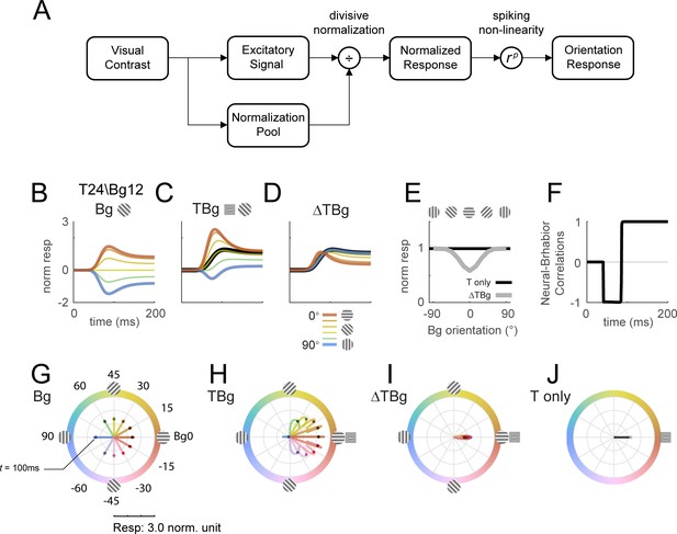
Delayed normalization model qualitatively captures key orientation masking response features.
(A) Schematic of the normalization model showing the visual input being processed by separate excitatory and normalization signal pathways. The normalization pathway in particular was modeled with a slightly delayed temporal kinetics and wider orientation tuning curves. The excitatory signal undergoes divisive normalization prior to neural output. (B–D) Modeled columnar response output with target contrast of 24% and background contrast of 12%. Modeled response normalized to the target only response averaged over 50–200ms as plotted in (E). (B) Modeled response of oriented backgrounds as in Figure 5A. (C) Modeled response of background with additive target as in Figure 5B, and the modeled response of the small Gabor target in black. (D) The target evoked response was obtained by subtracting the background only response (B) from (C), matching the biphasic observation in Figure 5C. (E) Model response integrated over 50–200ms in the same format as Figure 5D. (F) Correlation of modeled behavioral performance (Gaussian fit in Figure 5L) against each time frame of the modeled response, illustrating the early phase where the response was negatively correlated to behavioral choice, and the late phase with positive correlations. (G–J) Modeled time course of the population tuning vector. (G) Modeled populating tuning trajectory of the background only stimuli (color coded) as in Figure 7B. (H) Modeled populating tuning trajectory of the background with additive target illustrating the turn towards a convergent point on the x-axis as in Figure 7C. (I) Modeled target evoked response trajectory from subtracting (F) from (G). (J) Modeled populating tuning trajectory of the target only trials as in Figure 7E.
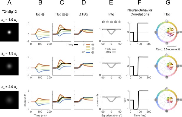
Divisive normalization model with different normalization spatial extents.
The spatial extent of the normalization kernel was varied to determine its effect on key model outputs from Figure 8. The size of sn was varied while all other parameters were at the same values as in Figure 8. Target contrast was modeled at 24% and background contrast at 12% (as in Figure 5G–L). (A) Illustration of the size of the normalization spatial kernel. Figure 8 was simulated with sn = 0.28° (row 1). (B–D) Model response corresponding to Figure 8B–D. (E) Model response integrated over 50–200ms in the same format as Figure 8E. (F) Correlation of modeled behavioral performance (Gaussian fit in Figure 5L) against each time frame of the modeled response. (G) Modeled populating tuning trajectory corresponding to Figure 8H.
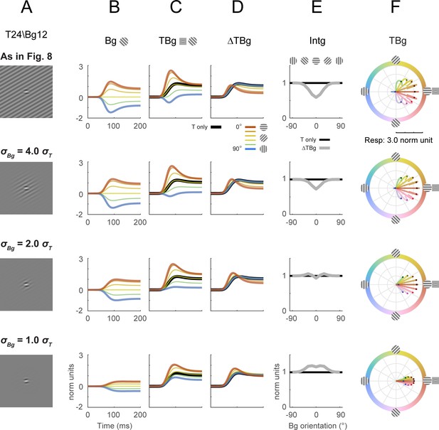
Divisive normalization model with different background spatial extents.
The spatial extent of the background grating (σBg) was explored for its effect on key model outputs from Figure 8 (row 1). The size of σBg was varied while all other parameters were at the same values as in Figure 8. Target contrast was modeled at 24% and background contrast at 12% (as in Figure 5G–L). (A) Illustration of the additive Gabor target on the background grating. Figure 8 was with a full field, uniform contrast grating covering the entire square simulation area (row 1). To simulate different background sizes, a Gaussian mask was applied co-centric to the target and with a spatial σBg relative to the size of the target (σT) as labeled. (B–D) Model response corresponding to Figure 8B–D. (E) Model response integrated over 50–200ms in the same format as Figure 8E. (F) Modeled populating tuning trajectory corresponding to Figure 8H.
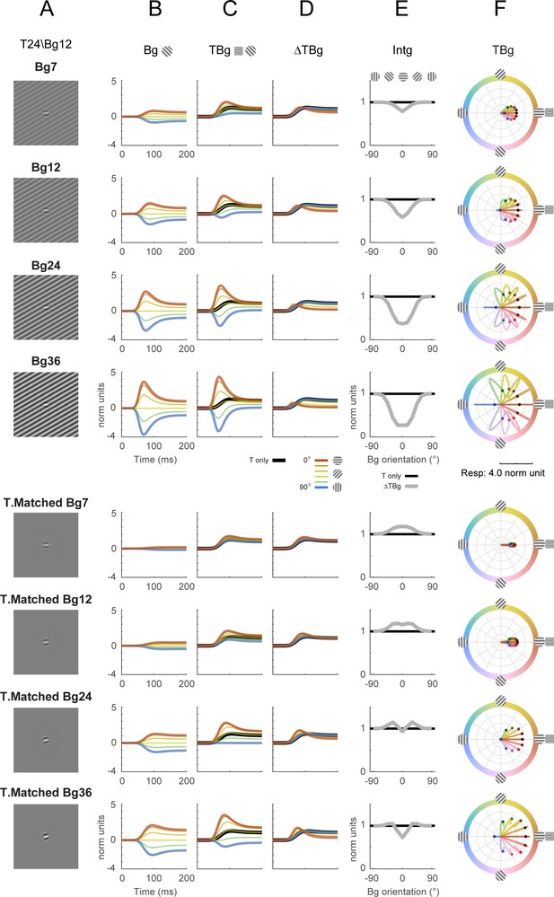
Divisive normalization model with different background contrasts.
The contrast level of the background grating was explored for its effect on key model outputs from Figure 8 (row 2). Rows 1–4: The contrast of the background was varied while all other parameters were at the same values as in Figure 8. Rows 5–8: Contrast of background was varied with the background set to the same size as the Gabor target, while all other parameters were at the same values as in Figure 8. Target contrast was 24% for all rows (as in Figure 8), and the background contrast for each row is as labeled. (A) Illustration of the additive Gabor target on the background grating. (B–D) Model response corresponding to Figure 8B–D. (E) Model response integrated over 50–200ms in the same format as Figure 8E. (F) Modeled populating tuning trajectory corresponding to Figure 8H.
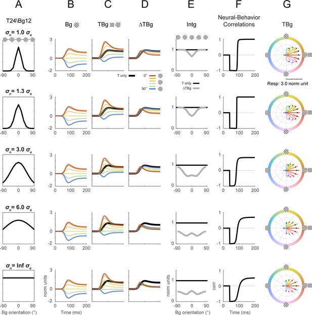
Divisive normalization model with different normalization signal orientation tuning width.
The orientation tuning width (σn) of the normalization signal was explored for its effect on key model outputs from Figure 8. The size of σn was varied while all other parameters were at the same values as in Figure 8. Target contrast was modeled at 24% and background contrast at 12% (as in Figure 5G–L). (A) Illustration of the normalization signal orientation tuning. Figure 8 was simulated with σe = 15° and σn = 20° (row 1). (B–D) Model response corresponding to Figure 8B–D. (E) Model response integrated over 50–200ms in the same format as Figure 8E. (F) Correlation of modeled behavioral performance (Gaussian fit in Figure 5L) against each time frame of the modeled response. (G) Modeled populating tuning trajectory corresponding to Figure 8H.
Tables
Experiment summary.
Experiment counts and the total number of trials included in the analysis presented in Figures 2, 4, 5 and 7; Figure 4—figure supplements 1 and 2; and Figure 5—figure supplement 1. Experiments with ineffective VSD staining were excluded from # Experiments. Trials with excessive motion or inconsistent EKG were excluded from # Total trials. Age of monkey reported at the time of the last listed experiment.
| Target Contrast | Background Contrast | # Experiments | # Total Trials | # Hits | # Misses | # Correct Rejects (CR) | # False Alarms (FA) | |
|---|---|---|---|---|---|---|---|---|
| Monkey H Male 8 years old | T12% | --- | 5 | 52 | 26 | 0 | 25 | 1 |
| T12% | Bg7% | 3 | 593 | 214 | 80 | 253 | 46 | |
| T12% | Bg12% | 2 | 397 | 125 | 74 | 121 | 77 | |
| Monkey T Male 7 years old | T12% | --- | 11 | 490 | 185 | 59 | 228 | 18 |
| T12% | Bg7% | 5 | 1660 | 644 | 189 | 740 | 87 | |
| T12% | Bg12% | 6 | 1748 | 704 | 169 | 683 | 192 | |
| T24% | --- | 16 | 546 | 272 | 0 | 267 | 7 | |
| T24% | Bg7% | 5 | 1012 | 501 | 5 | 450 | 56 | |
| T24% | Bg12% | 6 | 1320 | 654 | 12 | 599 | 55 | |
| T24% | Bg24% | 4 | 388 | 204 | 2 | 155 | 27 |
| Reagent type (species) or resource | Designation | Source or reference | Identifiers | Additional information |
|---|---|---|---|---|
| Voltage-sensitive dye | RH1691; RH1838 | Optical Imaging Inc. | RH1691; RH1838 |
Additional files
-
Supplementary file 1
Supplementary perceptual masking demonstration.
- https://cdn.elifesciences.org/articles/89570/elife-89570-supp1-v2.pdf
-
MDAR checklist
- https://cdn.elifesciences.org/articles/89570/elife-89570-mdarchecklist1-v2.pdf


