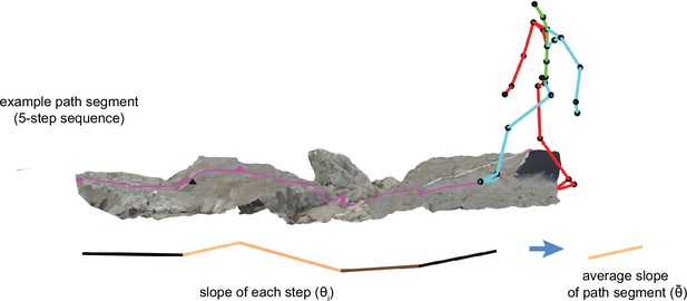
Analysis of foothold selection during locomotion using terrain reconstruction
Figures

Example comparison of original and rendered video frames.
We used the scene videos recorded by the eye tracker’s outward-facing camera to estimate the structure of the environment and the scene camera’s pose in each frame of the video. By moving a virtual camera to those poses and rendering the camera’s view of the textured mesh, we can generate comparison images to help assess the reconstruction’s accuracy. (A) Frame from original scene video. (B) Corresponding rendered image.
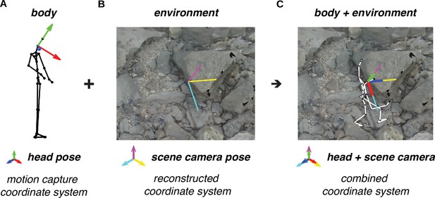
Alignment of motion capture data and terrain reconstruction.
We combine the motion capture data with the reconstructed environment (photogrammetry data) by aligning the head’s pose (RGB axes) to the scene camera’s pose (CMY axes). (A) Motion capture data provides body pose (i.e. position and orientation) information, including the head’s pose (RGB axes). (B) The process of reconstructing the environment via photogrammetry produces a three-dimensional (3D) terrain mesh (image) and scene camera’s poses (CMY axes). (C) Aligning the head’s pose (RGB axes) to the scene camera’s pose (CMY axes) places the body within the terrain reconstruction.
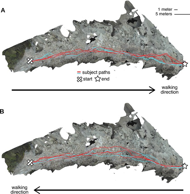
Repeated walks across rough terrain in the Austin data.
Each of the two Austin subjects walked out and back over a rocky trail three times. These overhead views show the textured three-dimensional (3D) terrain mesh along with the paths the subjects took through that terrain. Each color (red and cyan) corresponds to a different subject. Note that in some sections of the terrain, paths were highly similar across repetitions and across subjects, while in other sections, paths differed notably. (A) Both subjects’ three walks from the start of the path to the end. (B) Both subjects’ three walks returning to the start location.
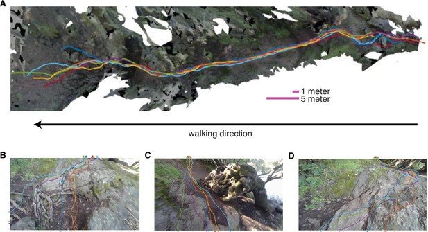
Berkeley path consistency, convergence and divergence.
(A) Overhead view of paths taken (colored lines correspond to individual subjects) through a portion of the Berkeley terrain. (B–D) These panels show examples of path convergence and divergence. The colored lines indicate the paths that subjects traveled in this section of the terrain, with each color representing a different subject. For each path, the walk in this section of terrain begins at the tick mark near the bottom of the image and ends at the colored In (B), subjects diverge by choosing two different routes around a root, but then converge again. In (C) subject paths converge to avoid the large outcrop. In (D) subject paths converge around a mossy section of a large rock.
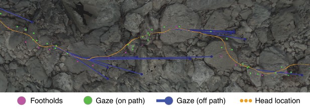
Gaze and body data embedded in the corresponding reconstructed terrain.
This overhead view shows a representative excerpt of 20 steps from one of the Austin traversals. The walker was, in this overhead view, moving left to right. Dots mark the footholds locations (pink), gaze locations near the path (green), gaze locations off the path (blue), and head locations (orange). To illustrate the relationship between ‘off-the-path‘ gaze and head location, blue lines connect each blue gaze point to the simultaneous location of the head.
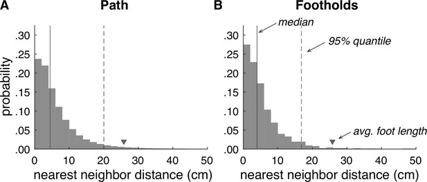
Accuracy of terrain reconstructions.
(A) Nearest neighbor error distribution for the whole terrain (median = 4.5 cm, 95% quantile = 20.0 cm). (B) Nearest neighbor error distribution for individual footholds (median = 4.0 cm, 95% quantile = 16.8 cm).
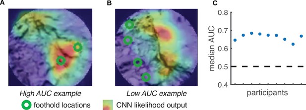
Predicting foothold locations from depth information.
A convolutional neural network (CNN) was trained to predict foothold locations in retinocentric depth images. (A) Example retinocentric depth image associated with relatively good CNN performance (i.e. a high area under the ROC curve [AUC] value). The image is overlaid with the foothold locations (green) and a heatmap showing the CNN’s likelihood output, which indicates the likelihood of finding a foothold in a particular location. (B) Example retinocentric depth image associated with relatively poor CNN performance (i.e. a low AUC value). (C) Median AUC values for the data of each of the nine participants.
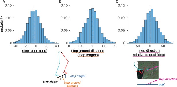
Step parameter distributions help define feasible alternative paths.
The histograms show the distributions of (A) step slopes, (B) step lengths, and (C) step direction relative to goal direction. These distributions define the set of feasible next steps for a given foothold, allowing the calculation of feasible alternative paths to the one actually chosen by the subject. This figure shows histograms of these quantities pooled over subjects, but note that calculations of viable paths were done based on the step parameters of each individual subject.
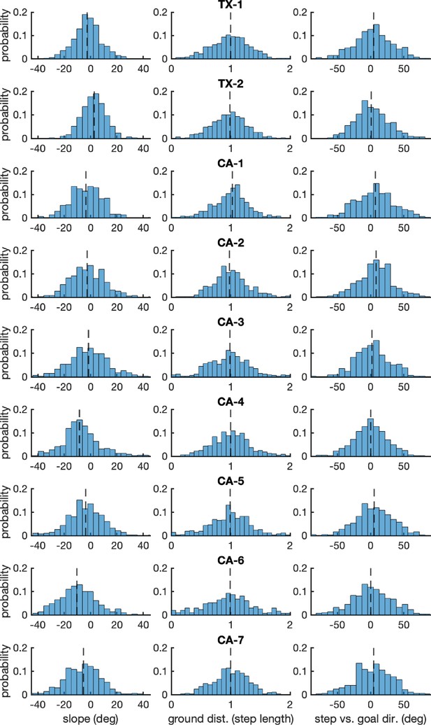
Per-subject histograms of the step parameters shown in Figure 7.
Each row shows one subject’s data. Each column shows data for one of the step parameters used to constrain simulated steps: (1) step slope, (2) step length normalized by the average step length, and (3) step direction relative to goal direction.
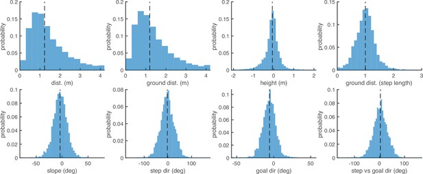
Aggregate histograms of the step parameters defined in the Methods section titled ‘Step analysis‘.
Top row, from left to right: (1) step distance (m), (2) step ground distance (m), (3) step height (m), (4) step ground distance (step length; see also Figure 7B). Bottom row: (1) step slope (deg; see also Figure 7A), (2) step direction (deg), (3) goal direction (deg), (4) step direction relative to goal direction (deg; see also Figure 7C).
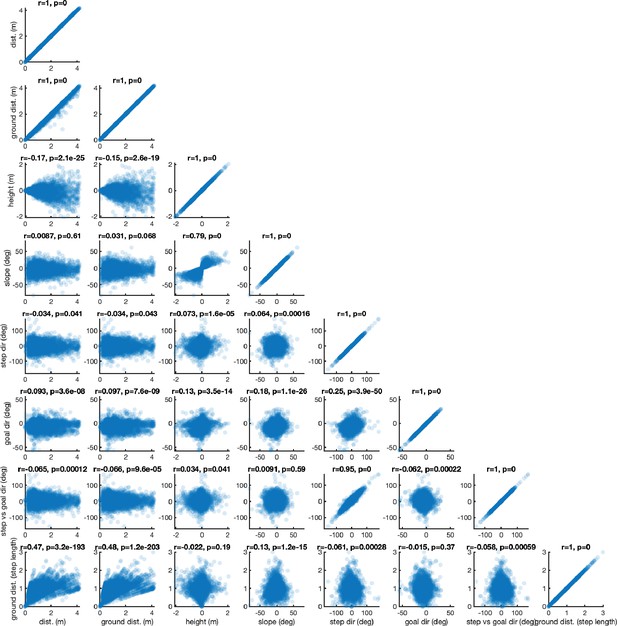
Scatterplots between all parameters defined in the Methods section titled ‘Step analysis‘.
The order of the step parameters along the x- and y-subplot axes are: (1) step distance, (2) step ground distance, (3) step height, (4) step slope, (5) step direction, (6) goal direction, (7) step direction relative to goal direction, and (8) step ground distance in step lengths. The title of each subplot contains the correlation value r and its associated p-value.
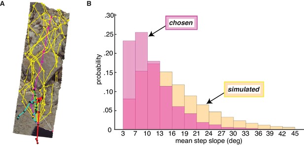
Paths chosen by walkers have a lower step slope.
We simulated path segments composed of viable steps and compared them to subjects’ chosen step sequences. (A) Overhead view of an example chosen step sequence (magenta), along with a subset of the corresponding simulated viable step sequences (yellow). The cyan and red lines show the walker’s skeleton. (B) Histograms of mean step slope for chosen and simulated step sequences for one participant.
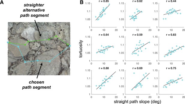
Average tortuosity of chosen path increases with increased straight path slope.
(A) An example chosen path segment (cyan; 5-step sequence), along with one straighter alternative path segment (green). (B) An illustration of the relationship between chosen path segment tortuosity and the slope of ‘straight’ path segments that were simulated across the same terrain. Each subpanel depicts one subject’s data. To summarize the large amount of data per subject (317,497 path segments), we binned the data into 20 quantiles of straight path slope and averaged tortuosity per bin, generating one summary tortuosity value per slope level. These scatterplots show the average tortuosity as a function of the straight path slope quantile (cyan crosses), along with best fit lines (black). (For scatterplots showing data per chosen path segment, see Figure 9—figure supplement 1A). Associated correlation values (Pearson’s r) are shown at the top of each panel.
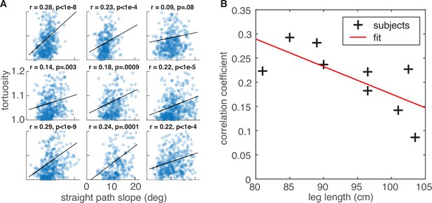
Relationship between average straight path segment slope and the tortuosity of each chosen path segment.
(A) Tortuosity of the chosen path segments (5-step sequences) vs. slope for the simulated ‘straight‘ path segments for each of the nine subjects. Correlation values and corresponding p-values are indicated at the top of each panel. (B) Correlation between subject leg length and the strength of the straight path slope vs. tortuosity relationship in their foothold selection data. Leg lengths (in cm) are plotted on the horizontal axis, and the correlation coefficients for each of the plots in panel A are plotted on the vertical axis. We found a statistically significant negative correlation between those two values (r = –0.70, p=0.04).

Distributions of straight path slope and chosen path segment tortuosity.
Each row presents one subject’s data. The left column contains histograms of the average slope for simulated ‘straight‘ path segments, and the right column contains histograms of the tortuosity of that subject’s chosen path segments (5-step sequences).
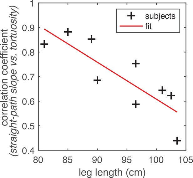
Relationship between leg length and the correlation between straight path step slope and path tortuosity.
Subjects’ leg lengths (in cm) are plotted on the horizontal axis. The correlation coefficients drawn from the analyses depicted in Figure 9B are plotted on the vertical axis. The scatterplot shows one point per subject (black crosses). The linear trendline is also shown (red line). We found that there was a statistically significant negative correlation between subjects’ leg lengths and the straight path slope vs. average path tortuosity correlations in their data (r=–0.83, p=0.005). (For a comparable plot showing the correlations derived from data per chosen path segment, see Figure 9—figure supplement 1B).

Convolutional neural network (CNN) inputs and outputs.
Schematic shows the inputs and outputs for one example frame. (A) Input: retinocentric depth image. (B) Target output: foothold likelihood map. (C) Output: predicted foothold locations.
Videos
Visualization of the aligned motion capture, eye tracking, and terrain data for one traversal of the Austin trail: https://youtu.be/TzrA_iEtj1s.
The video shows the three-dimensional (3D) motion capture skeleton walking over the textured mesh. Gaze vectors are illustrated as blue lines. On the terrain surface, the heatmap shows gaze density, and the magenta dots represent foothold locations.
Visualization of foothold locations in the scene camera’s view for one traversal of the Austin trail: https://youtu.be/llulrzhIAVg.
Computed foothold locations are marked with cyan dots.
Tables
Information about participants included in dataset.
Table includes the location of data collection, key demographics, and the amount of data recorded per participant (quantified as the number of steps in rough terrain in participants’ processed data).
| Location | TX | TX | CA | CA | CA | CA | CA | CA | CA |
|---|---|---|---|---|---|---|---|---|---|
| Age | 23 | 25 | 27 | 39 | 34 | 29 | 24 | 24 | 54 |
| Gender | F | M | M | M | M | F | F | F | M |
| Leg length (cm) | 89 | 102.5 | 103.5 | 101 | 96.5 | 81 | 85 | 90 | 96.5 |
| Step count | 468 | 347 | 462 | 489 | 385 | 537 | 486 | 603 | 453 |
Layers of custom convolutional neural network (CNN).
| Layer | Output shape | # Params |
|---|---|---|
| Conv2D | (100, 100, 4) | 404 |
| BatchNormalization | (100, 100, 4) | 16 |
| MaxPooling2D | (50, 50, 4) | 0 |
| Conv2D | (50, 50, 8) | 3208 |
| BatchNormalization | (50, 50, 8) | 32 |
| MaxPooling2D | (25, 25, 8) | 0 |
| Conv2D | (25, 25, 16) | 12,816 |
| BatchNormalization | (25, 25, 16) | 64 |
| Conv2DTranspose | (25, 25, 16) | 25,616 |
| BatchNormalization | (25, 25, 16) | 64 |
| UpSampling2D | (50, 50, 16) | 0 |
| Conv2DTranspose | (50, 50, 8) | 12,808 |
| BatchNormalization | (50, 50, 8) | 32 |
| UpSampling2D | (100, 100, 8) | 0 |
| Conv2DTranspose | (100, 100, 4) | 3204 |
| Conv2DTranspose | (100, 100, 1) | 401 |
| BatchNormalization | (100, 100, 1) | 4 |
| Flatten | (10,000) | 0 |
| Softmax | (10,000) | 0 |
| Reshape | (100, 100) | 0 |


