Microprism-based two-photon imaging of the mouse inferior colliculus reveals novel organizational principles of the auditory midbrain
- Department of Molecular and Integrative Physiology, University of Illinois at Urbana Champaign, United States
- Beckman Institute for Advanced Science and Technology, University of Illinois at Urbana Champaign, United States
- School of Molecular & Cell Biology, University of Illinois at Urbana-Champaign, United States
- Neuroscience Program, University of Illinois at Urbana-Champaign, United States
- Carle Illinois College of Medicine, University of Illinois at Urbana-Champaign, United States
Figures
Figure 1
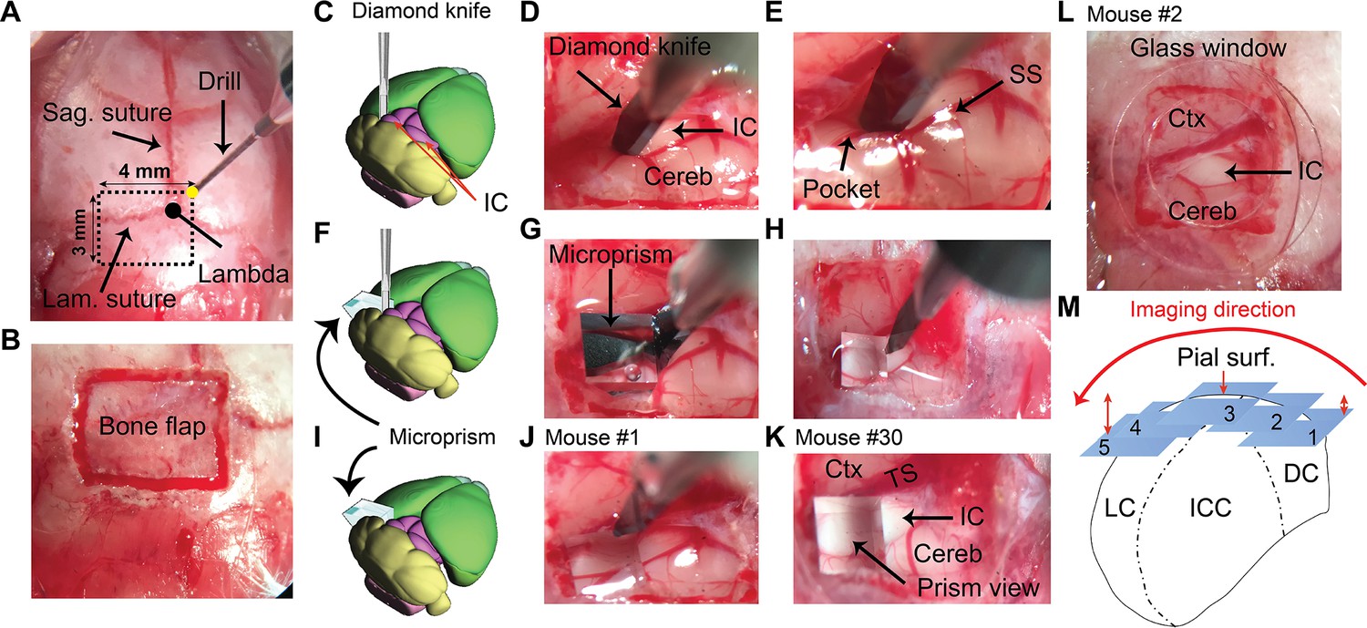
A brief illustration of the surgical procedures.
(A) A surface view of the mouse’s skull showing the landmarks of the craniotomy over the IC. (B) An image of the bone flap after finishing the drilling. (C–E) A cartoon and two images of the brain surface showing the insertion and the pocket made by the diamond knife at the lateral surface of the left IC. (F–H) A cartoon and two images of the brain surface show the insertion of the microprism into its pocket to directly face the LC after displacing the blade of the diamond knife. (I–K) A cartoon and two images of the brain surface show the final setup of the microprism for two different animals. (L) An image of the brain surface shows the placement of a glass window for the surface imaging of the DC. (M) A cartoon of the coronal section of the IC demonstrating the different fields of views taken along the mediolateral axis parallel to the curvature of the IC surface at different depths (1–5) from the pial surface. Cereb: cerebellum, Ctx: cerebral cortex, DC: dorsal cortex of the IC, IC: inferior colliculus, ICC: central nucleus of the IC, Lam.: lambdoid, LC: lateral cortex of the IC, Sag.: sagittal, SS: sigmoid sinus, Surf: surface, TS: transverse sinus.
Figure 2
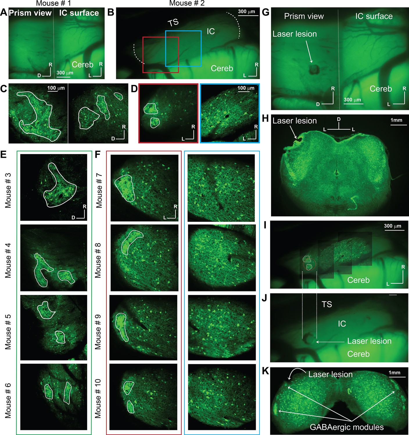
The distribution of GABAergic cells on the LC(microprism) and DC imaged from the dorsal surface.
All images were taken for the GFP signals exclusively expressed in GABAergic cells. (A, B) Low magnification of fluorescence images for the GFP signals obtained from the IC surface with or without the microprism, respectively. The dotted white line in B represented the medial and lateral horizons of the IC. (C, E) The two-photon (2P) images of the GABAergic cells on the LC(microprism) show the GABAergic modules across multiple animals. (D, F) The 2P images of the GABAergic cells on either the dorsolateral surface of the DC imaged directly from its dorsal surface showing the GABAergic modules across multiple animals (red boxes) or its dorsomedial surface showing a homogenous distribution of GABAergic cells of different sizes with no signs of the GABAergic modules across multiple animals (blue boxes). (G) A low-magnification fluorescence image of the IC surface with the microprism showing a laser lesion spot made through the microprism to validate the position of the microprism relative to the IC. (H) A histological coronal section at the level of the IC shows that the laser lesion made by the microprism was located at the sagittal surface of the LC(microprism). (I–J) Low-magnification fluorescence images of the IC surface from the dorsal surface show a laser lesion spot made on the dorsolateral surface of the LC on the GABAergic module. The dotted white lines represent the alignment of the laser lesion (dotted red circle) to the location of the GABAergic module at the dorsolateral surface. (K) A histological coronal section at the level of the IC shows that the laser lesion made on the IC surface targeted the GABAergic module at the dorsolateral portion of the LC. All solid irregular white lines were made at the border of the GABAergic modules. D: dorsal, IC: inferior colliculus, L: lateral, R: rostral, Cereb: cerebellum, TS: transverse sinus.
Figure 3 with 1 supplement
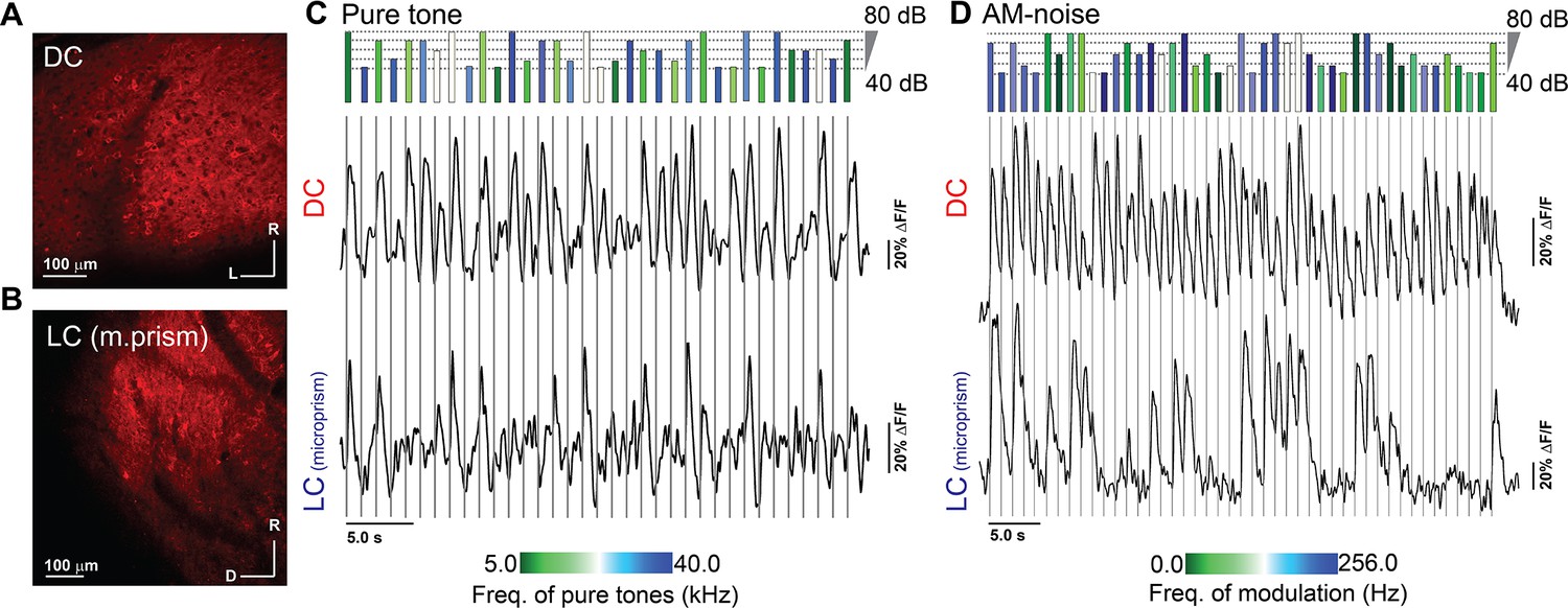
Two-photon (2P) expression of jRGECO1a along with evoked signals in the DC imaged from the dorsal surface and LC(microprism).
(A, B) The 2P images of the jRGECO1a expression on the DC imaged from the dorsal surface and the LC(microprism), respectively. (C, D) The time traces of the evoked calcium signals by either different frequencies and amplitudes of pure tones or different overall amplitudes and rates of AM of broadband noise, respectively, which were obtained from two different cells on the DC (top traces) or the LC(microprism) (bottom traces). The length of the colored bars (top) indicates the intensity of the stimulus, while the color indicates the tone or AM frequency depending on the color scale (bottom). AM-noise: amplitude modulated broadband noise, D: dorsal, DC: dorsal cortex, L: lateral, LC: lateral cortex, R: rostral.
Figure 3—figure supplement 1
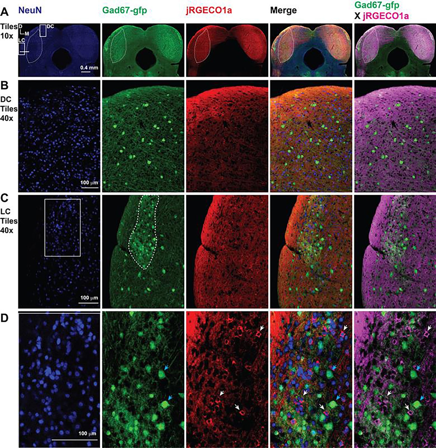
The expression of jRGECO1a in the IC across different regions and cell types.
(A) Image of the inferior colliculus (IC) showing the immunostaining to NueN (blue-column 1), GAD67-GFP (green-column 3), jRGECO1a (red-column 3), merged image for the three proteins (column 4), and merged image for jRGECO1a (magenta) and GFP (green) – dotted lines represent the central nucleus of the IC in all channels as well as the modules in the green channel. (B) A magnified view of the dorsal cortex (DC) in A – dotted line represents the central nucleus of the IC (ICC). (C) A magnified view of the lateral cortex (LC) in A – dotted line represents one of the GABAergic modules of the LC. (D) A magnified view of the white square in C shows some GABAergic cells (blue arrows) and some non-GABAergic cells expressing jRGECO1a (white arrows). D: dorsal, L: lateral.
Figure 4 with 1 supplement
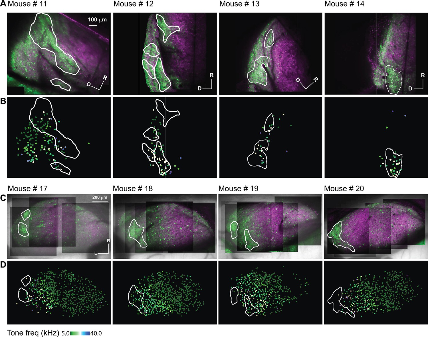
The auditory cellular organization of the LC(microprism) vs dorsal cortex (DC) imaged from the dorsal surface.
(A, C) The two-photon (2P) images of GFP (green) and jRGECO1a expression (red) on either the LC(microprism) or the DC imaged from the dorsal surface, respectively. (B, D) The pseudocolor images show the responsive cells to the pure tone of different combinations of frequencies and levels on the surface of the LC(microprism) or the DC imaged from its dorsal surface, respectively. D: dorsal, L: lateral, R: rostral.
Figure 4—figure supplement 1
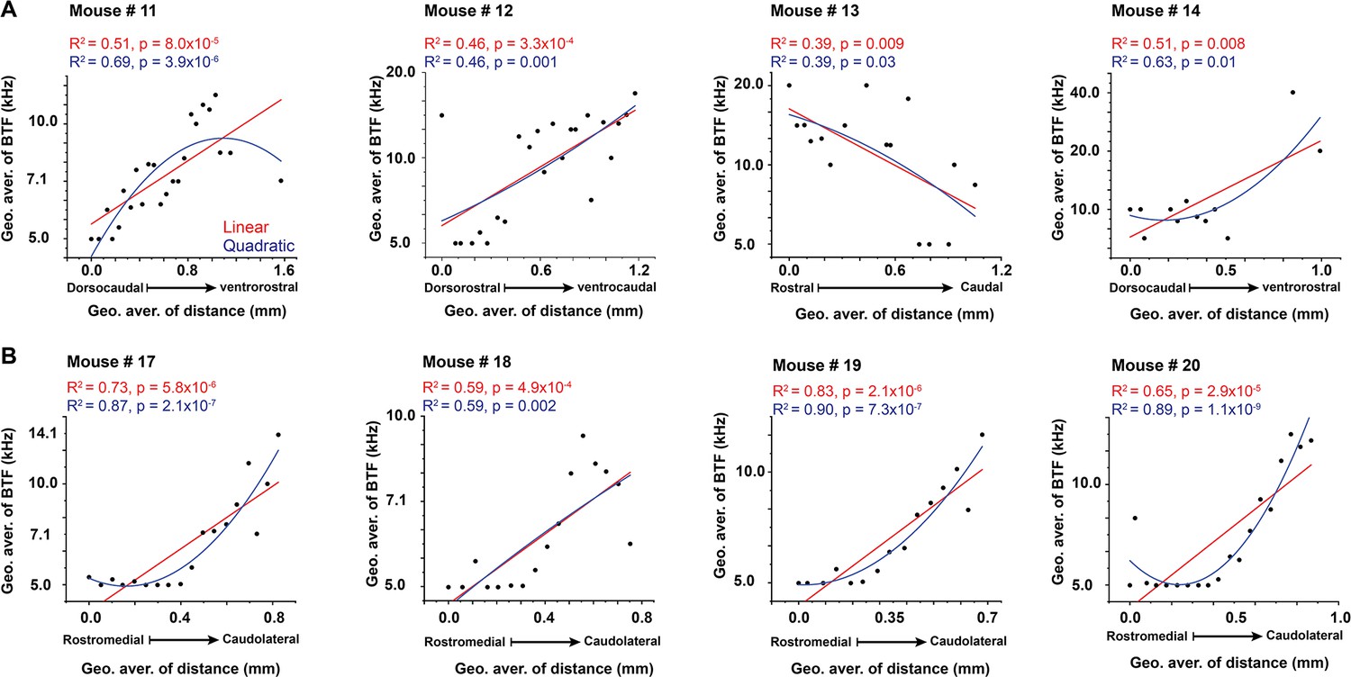
The best regression fit between best tone frequency and different anatomical axes.
(A, B) Linear and nonlinear quadratic regression fit between the best pure tone frequencies (BTFs) and the locations of the cells of the LC(microprism) and the dorsal cortex (DC), respectively.
Figure 5
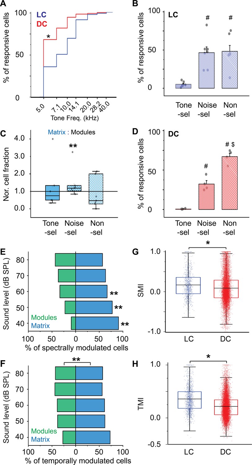
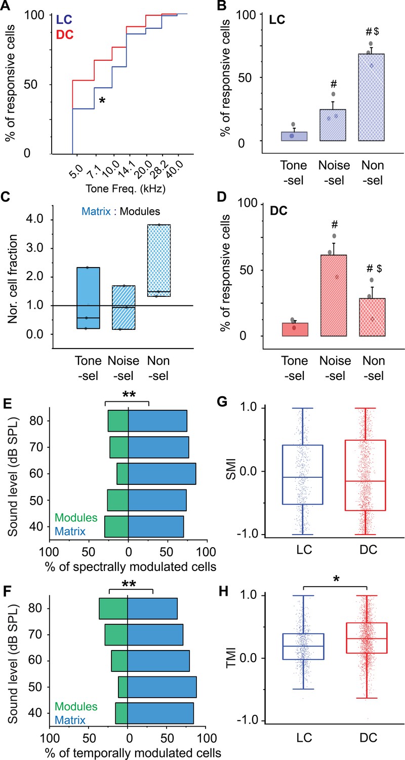
The cellular response to pure tones and AM-noise of the LC(microprism) vs DC imaged from the dorsal surface.
(A) The cumulative distribution function of the best tone frequencies of all cells collected either from the LC imaged via microprism (blue line) or the DC imaged directly from its dorsal surface (red line) (Mann-Whitney test: z=–11.34, p<0.001, a median of best-tuned frequency = 5 and 7.1 Hz for the DC (2484 cells from 4 animals) and the LC(microprism) (445 cells from 7 animals), respectively, *p<0.05, DC vs LC(microprism)). (B) A bar graph showing the fractions of cells responding to only pure tone (Tone-sel), only AM-noise (Noise-sel), or to both nonselectively (Non-sel) on the LC(microprism) (7 animals) (one-way ANOVA, f(2,18) = 14.9, p=1.6 × 10⁻⁴, Fisher’s post hoc test: p=2.0 × 10⁻⁴ and 1.3×10⁻⁴ for Noise-sel and Non-sel vs Tone-sel, respectively, p=0.84 for Noise-sel vs Non-sel, % of responsive cells ± SEM = 5 ± 1%, 46 ± 7%, and 48 ± 7% for Tone-sel, Noise-sel, and Non-sel, respectively, #p<0.05 vs Tone-sel). (C) Box graphs showing the fractions of Tone-sel, Noise-sel, and Non-sel cells within modules and matrix of the LC(microprism). (D) A bar graph showing the fractions of Tone-sel, Noise-sel, or Non-sel cells on the DC imaged directly from the dorsal surface (4 animals) (one-way ANOVA, f(2,9) = 86.9, p=1.2 × 10⁻⁶, Fisher’s post hoc test: p=1.5 × 10⁻⁴ and 3.4×10⁻⁷ for Noise-sel and Non-sel vs Tone-sel, respectively, p=7.0 × 10⁻⁵ for Noise-sel vs Non-sel, % of responsive cells ± SEM = 0.6 ± 0.2%, 32 ± 4%, and 67 ± 4% for Tone-sel, Noise-sel, and Non-sel, respectively, #p<0.05 vs Tone-sel and $p<0.05 vs Noise-sel). (E, F) Bar graphs showing the percentage of spectrally (two-way ANOVA: f(1, 4, 20)=50.3, 0.0, and 4.0 – p=7.1 × 10⁻⁷, 1.0, and 0.01 for the region, sound level, and interaction, respectively, Fisher’s post hoc, p=5.1 × 10⁻⁶, 4.9×10⁻⁴, 0.02, 0.058, and 0.14 for modules vs matrix at 40, 50, 60, 70, and 80 dB, respectively, % of spectral modulated cells ± SEM (modules vs matrix)=9 ± 1% vs 90 ± 1% at 40 dB, 22 ± 4% vs 77 ± 4% at 50 dB, 33±10% vs 66 ± 10% at 60 dB, 36 ±13% vs 63 ± 13% at 70 dB, and 43 ±11% vs 56 ± 11% at 80 dB, n=3 animals) or temporally (two-way ANOVA: f(1, 4, 20)=19.3, 0.0, and 1.2 – p=7.1 × 10⁻⁷, 1.0, and 0.32 for the region, sound level, and interaction, respectively, % of temporally modulated cells ± SEM = 38 ± 3% and 61 ± 3% for modules vs matrix, n=3 animals) modulated cells, respectively, across different sound levels in modules (green bars) vs matrix (blue bars) imaged via microprism (**p<0.05, matrix vs modules). (G, H) Box plots showing the mean (black lines) and the distribution (colored dots) of the SMI (two-way ANOVA: f(1, 4, 14583)=48.4, 210.4, and 21.3 – p<0.001 for the region, sound level, and interaction, respectively, Fisher’s post hoc test, p=6.2 × 10⁻⁴, 4.2×10⁻⁵, <0.001, and <0.001 for LC vs DC at 40, 60, 70, and 80 dB respectively, mean of SMI ± SEM: 0.16 ± 0.01 and 0.08 ± 0.003 for LC vs DC, n=1020 cells from 7 animals (LC(microprism)), and 13,574 cells from 4 animals (DC)) and TMI (two-way ANOVA: f(1, 4, 16139)=431.4, 59.1, and 8.3 – p<0.001 for the region, sound level, and interaction, respectively, Fisher’s post hoc test, p=0.002, <0.001, <0.001, <0.001, and <0.001 for LC vs DC at 40, 50, 60, 70, and 80 dB, respectively, mean of TMI ± SEM: 0.35 ± 0.006 and 0.21 ± 0.001 for LC vs DC, n=1441 cells from 7 animals (LC(microprism)), and 14,708 cells from 4 animals (DC)), respectively, across different sound levels in the LC(microprism) (blue) vs the DC (red), *p<0.05, LC vs DC. DC: dorsal cortex, LC: lateral cortex. SMI: spectral modulation index, TMI: temporal modulation index.
Figure 6
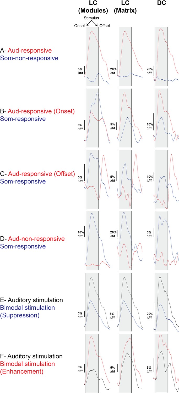
The waveforms of the somatosensory vs acoustic responses of the LC(microprism) and the dorsal cortex (DC) imaged via microprism.
Examples of different cell types based on their responses to auditory or somatosensory stimulations as well as their response timing to the auditory stimulation as indicated by waveforms of the evoked calcium signals.
Figure 7
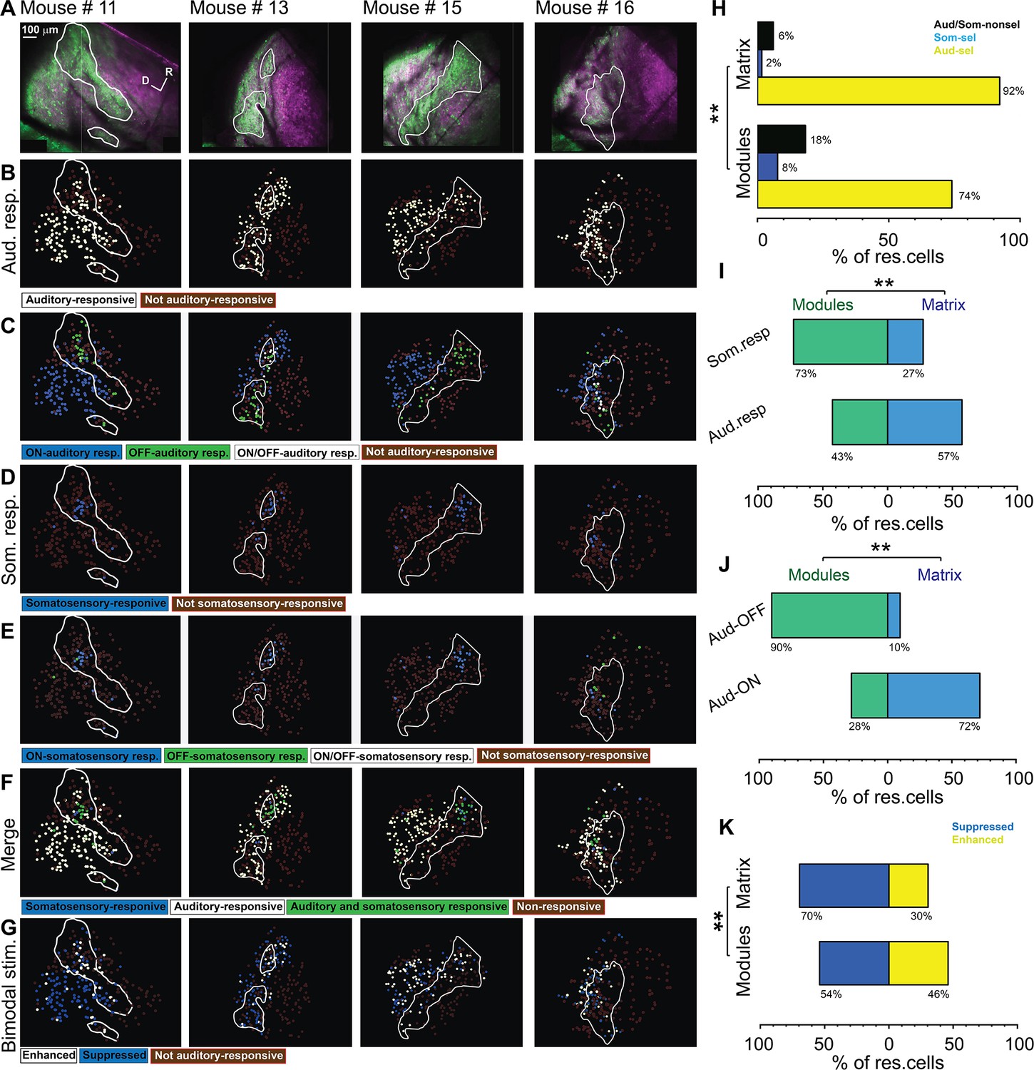
Types of somatosensory and auditory responses from the lateral cortex (LC) neurons imaged via microprism.
(A) The two-photon (2P) images of GFP (green) and jRGECO1a expression (magenta) in the LC(microprism) show the modules within white irregular lines. (B, D, F) The pseudocolor images show the auditory (white circles) or somatosensory (blue circles) responsive cells of the LC(microprism) as well as the merged response (green circles), respectively. (C, E) The pseudocolor images show onset (ON) (blue circles), offset (OFF) (green circles), or onset/offset (ON/OFF) (white circles) responsive cells of the LC(microprism) to auditory and somatosensory stimuli, respectively. (G) The pseudocolor images show enhanced (white circles) and suppressive response (blue circles) of the auditory responsive cells of the LC(microprism) following the bimodal stimulation based on their response index (RI). (H) A bar graph showing the percentage of responsive cells to auditory stimulation only or auditory selective cells (Aud-sel, yellow bars), to somatosensory stimulation only or somatosensory selective cells (Som-sel, blue bars), or nonselectively to both auditory and somatosensory stimulations (Aud/Som-nonsel, black bars) in modules vs matrix (chi-square test, χ2=33.1, p=3.5 × 10⁻⁶, % of responsive cells = 74%, 8%, and 18% for Aud-sel, Som-sel, and Aud/Som-nonsel, respectively at [modules, 235 cells] vs 92%, 2%, and 6% for Aud-sel, Som-sel, and Aud/Som-sel, respectively at [matrix, 297 cells] – 4 animals, **p<0.05 vs modules). (I) A bar graph showing the percentage of all cells having auditory responses (Aud. resp) or those having somatosensory responses (Som. resp) in modules vs matrix (chi-square test, χ2=26.0, p=9.3 × 10⁻⁵, % of responsive cells [modules vs matrix]=43% vs 57% for [Aud-resp, 509 cells] and 73% vs 27% for [Som. resp, 84 cells] – 4 animals, **p<0.05 vs modules). (J) A bar graph showing the percentage of auditory responsive cells with onset (Aud-ON) vs those with offset (Aud-OFF) responses in modules vs matrix (chi-square test, χ2=120.5, p<0.001, % of responsive cells [modules vs matrix]=28% vs 72% for [Aud-ON, 390 cells] and 90% vs 10% for [Aud-OFF, 93 cells] – 4 animals, **p<0.05 vs modules). (K) A bar graph showing the percentage of auditory responsive cells with suppressed vs those with enhanced responses following bimodal stimulation in modules vs matrix (chi-square test, χ2=12.9, p=0.04, % of responsive cells = 54% vs 46% for suppressed vs enhanced [modules, 217 cells] and 70% vs 30% for suppressed vs enhanced [matrix, 292 cells] – 4 animals, **p<0.05 vs modules). D: dorsal, R: rostral.
Figure 8
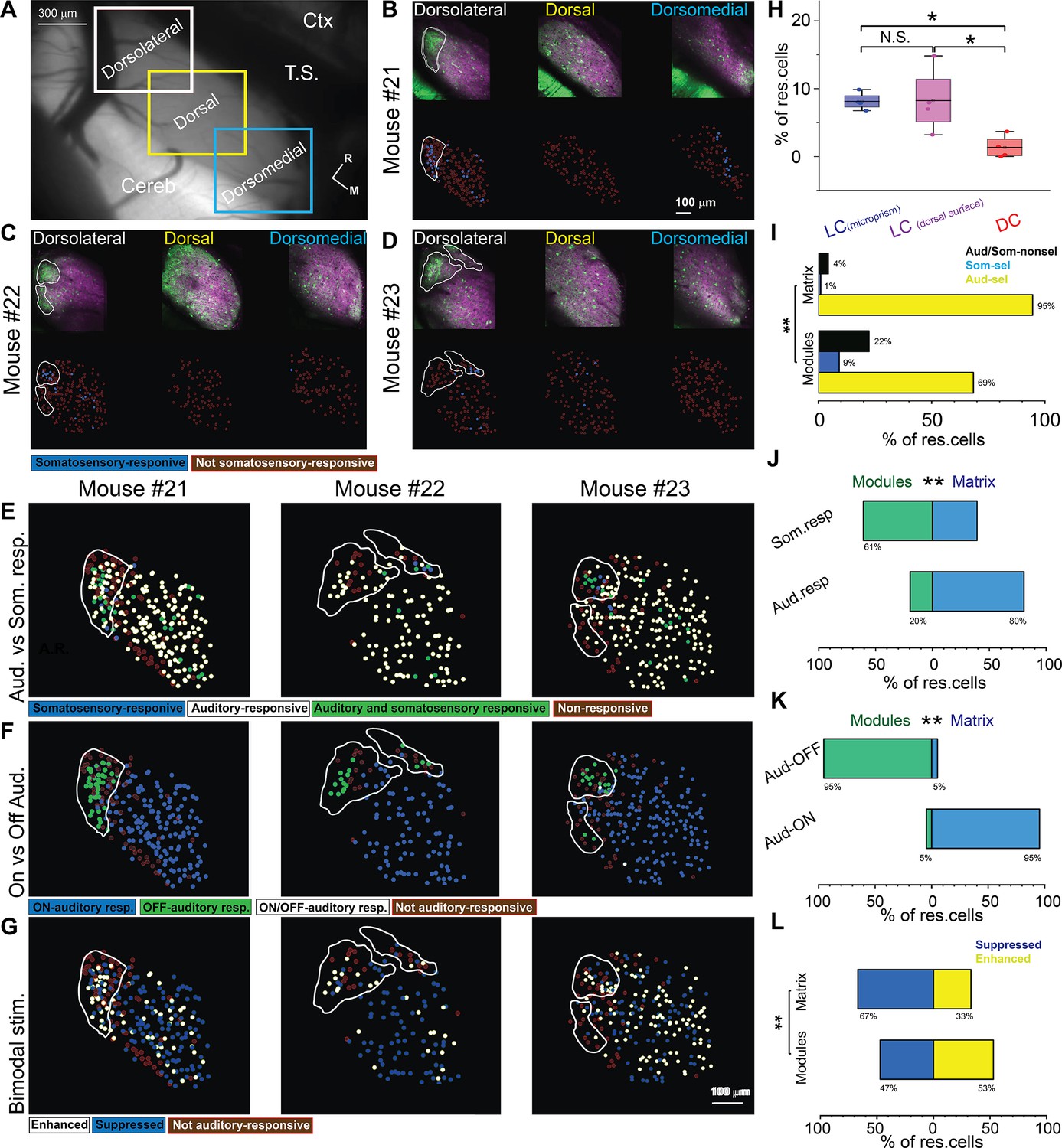
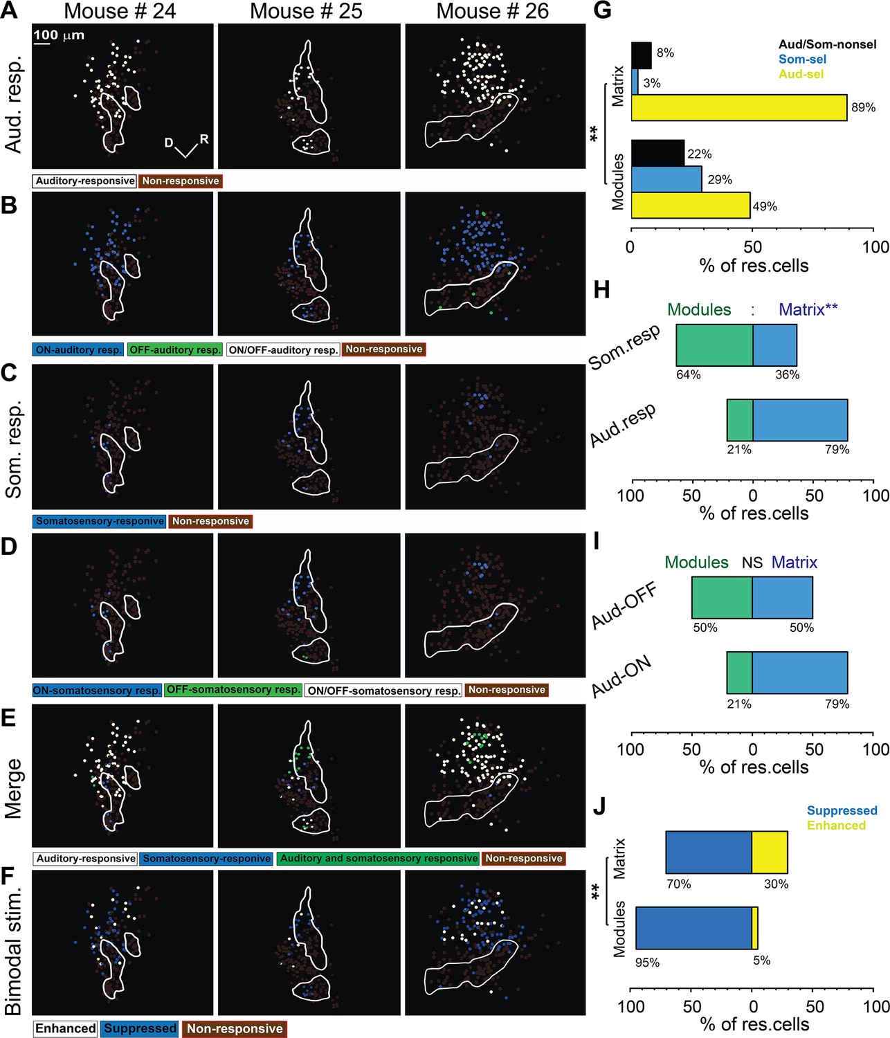
The somatosensory vs auditory responses over the dorsal cortex (DC) neurons.
(A) A low magnification of the image obtained from the inferior colliculus (IC) surface. (B–D) The top row: the two-photon (2P) images of GFP (green) and jRGECO1a expression (magenta) of three main regions (dorsolateral, dorsal, and dorsomedial) of the DC surface imaged from the dorsal surface showing the modules within irregular white lines in the dorsolateral region. The bottom row: the pseudocolor images show the somatosensory responsive cells (blue circles) after somatosensory stimulations. (E) The pseudocolor images show the responsive cells of the LC(dorsal surface) to auditory (white circles), somatosensory (blue circles), or both stimulations (green circles). (F) The pseudocolor images show auditory onset (Aud-ON – blue circles), offset (Aud-OFF, green circles), or onset/offset (Aud-ON/OFF, white circles) responsive cells of the LC imaged from the dorsal surface to auditory stimulation. (G) The pseudocolor images show the enhanced (white circles) and suppressive (blue circles) response of the auditory responsive cells of the LC imaged from the dorsal surface following the bimodal stimulation based on their response index (RI). (H) A box plot shows the percentage of somatosensory responsive cells in the LC(microprism), the LC(dorsal surface), or the DC (one-way ANOVA, p=0.02, the percentage of somatosensory responsive cells mean ± SEM = 1.3 ± 0.83% [DC, 4 animals, 8.2 ± 2.4%][LC(dorsal surface), 4 animals], and 8.1 ± 0.64% [LC(microprism), 4 animals, *p<0.05, vs DC]). (I) A bar graph showing the percentage of responsive cells to auditory stimulation only or auditory selective cells (Aud-sel, yellow bars), to somatosensory stimulation only or somatosensory selective cells (Som-sel, blue bars), or nonselectively to both auditory and somatosensory stimulations (Aud/Som-nonsel, black bars) in modules vs matrix (chi-square test, χ2=86.1, p<0.001, % of responsive cells = 69%, 9%, and 22% for Aud-sel, Som-sel, and Aud/Som-nonsel [modules, 152 cells] and 95%, 1%, and 4% for Aud-sel, Som-sel, and Aud/Som-nonsel [matrix, 573 cell] – 4 animals, **p<0.05 vs modules). (J) A bar graph showing the percentage of all cells having auditory responses (Aud. resp) or those having somatosensory responses (Som. resp) in modules vs matrix (chi-square test, χ2=66.5, p<0.001, % of responsive cells [modules vs matrix] = 20% vs 80% for [Aud. resp, 705 cells] and 61% vs 39% for [Som. resp, 79 cells] – 4 animals, **p<0.05 vs modules). (K) A bar graph showing the percentage of auditory responsive cells with onset (Aud-ON) vs those with offset (Aud-OFF) responses in modules vs matrix (chi-square test, χ2=500.2, p<0.001, % of responsive cells [modules vs matrix]=5% vs 95% for [Aud-ON, 584 cells] and 95% vs 5% for [Aud-OFF, 116 cells] – 4 animals, **p<0.05 vs modules). (L) A bar graph showing the percentage of auditory responsive cells with suppressed vs those with enhanced responses following bimodal stimulation in modules vs matrix (chi-square test, χ2=18.5, p=1.6 × 10⁻⁵, % of responsive cells = 47% vs 53% for suppressed vs enhanced [modules, 138 cells] and 67% vs 33% for suppressed vs enhanced [matrix, 567 cells] – 4 animals, **p<0.05 vs modules). Cereb: cerebellum, Ctx: cerebral cortex, M: medial, R: rostral, TS: transverse sinus.
Figure 9 with 1 supplement
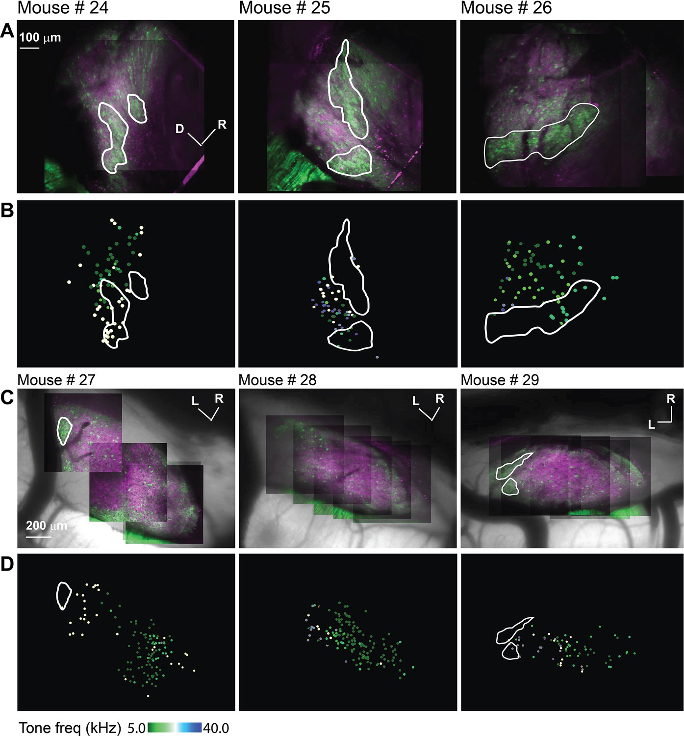
The acoustic response from LC(microprism) and dorsal cortex (DC) imaged from the dorsal surface in awake animals.
(A, C) The two-photon (2P) images of GFP (green) and jRGECO1a expression (magenta) on either the LC(microprism) surface imaged via the microprism or the DC imaged directly from the dorsal surface, respectively showing the modules within irregular white lines. (B, D) The pseudocolor images show the responsive cells to the pure tone of different combinations of frequencies and levels of the LC(microprism) or the DC imaged directly from the dorsal surface, respectively. D: dorsal, L: lateral, R: rostral.
Figure 9—figure supplement 1
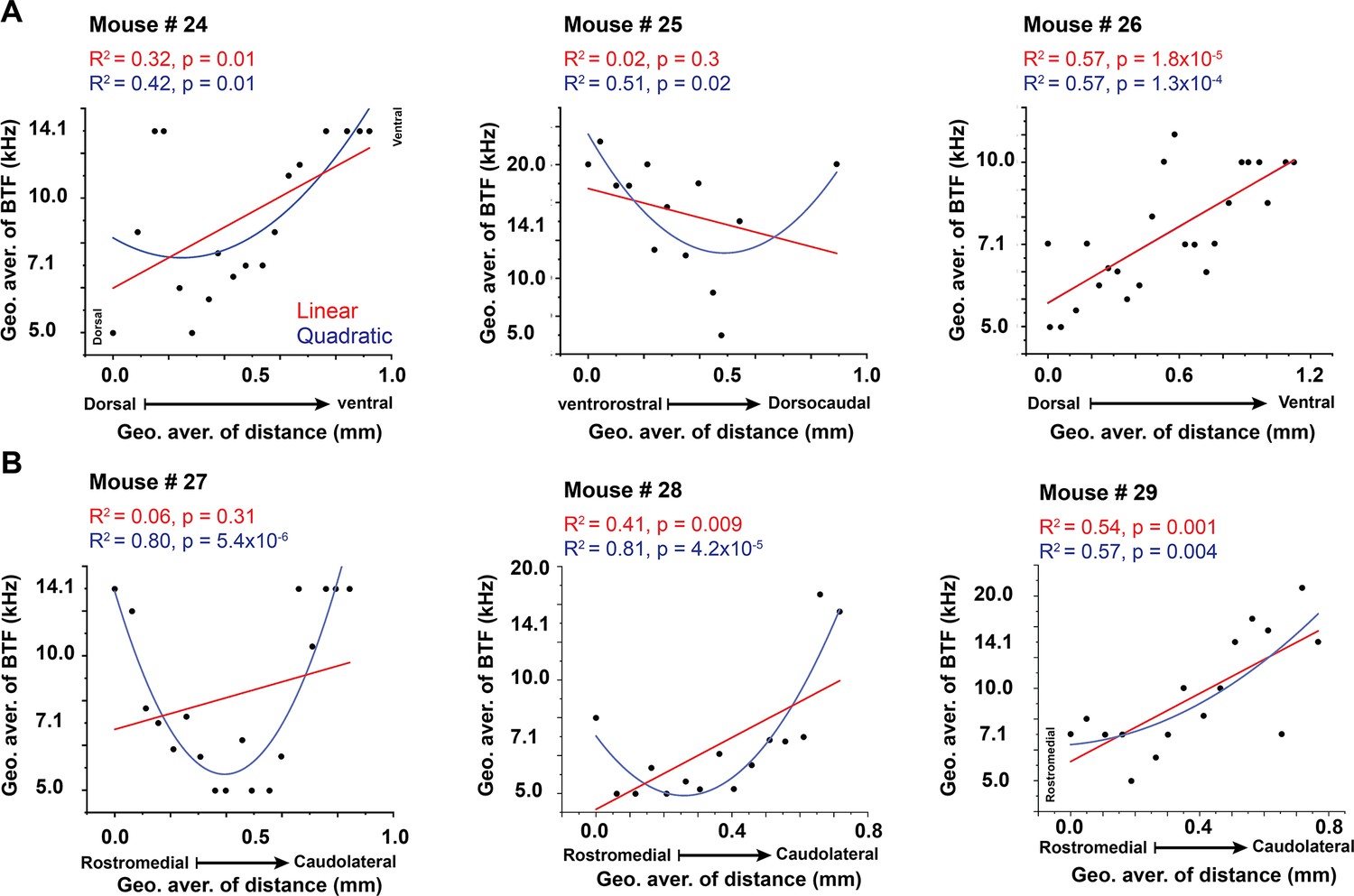
The best regression fit between best tone freuency and different anatomical axes.
(A,B) Linear and nonlinear quadratic regression fit between the best pure tone frequencies (BTFs) and the locations of the cells of the LC(microprism) and the dorsal cortex (DC), respectively.
Figure 10 with 1 supplement
The cellular response to pure tones and AM-noise of the LC(microprism) vs dorsal cortex (DC) imaged from the dorsal surface in awake animals.
(A) The cumulative distribution function of the best tone frequencies of all cells collected either from the lateral cortex (LC) imaged via microprism (blue line) or the DC imaged directly from its dorsal surface (red line) (Mann-Whitney test, z=–4.8, p=1.6 × 10⁻⁶, a median of best-tuned frequency = 5 and 10 kHz for the DC [767 cells from 3 animals] and the LC(microprism) [371 cells from 3 animals], respectively, *p<0.05 vs DC). (B) A bar graph showing the fractions of cells responding to only pure tone (Tone-sel), only AM-noise (Noise-sel), or to both nonselectively (Nonsel) on the LC(microprism) (3 animals) (one-way ANOVA, f(2,6) = 41.6, p=3.0 × 10⁻⁴, Fisher’s post hoc test: p=0.04 and 1.1×10⁻⁴ for Noise-sel and Non-sel vs Tone-sel, respectively, p=7.3 × 10⁻⁴ for Noise-sel vs Non-sel, % of responsive cells ± SEM = 6 ± 3%, 24 ± 6%, and 68 ± 5% for Tone-sel, Noise-sel, and Non-sel, respectively, #p<0.05 vs Tone-sel and $p<0.05 vs Noise-sel). (C) Box graphs showing the fractions of Tone-sel, Noise-sel, and Non-sel cells within modules and matrix of the LC(microprism). (D) A bar graph showing the fractions of Tone-sel, Noise-sel, or Non-sel cells on the DC imaged directly from the dorsal surface (3 animals) (one-way ANOVA, f(2,6) = 12.8, p=0.006, Fisher’s post hoc test: p=0.002 and 0.12 for Noise-sel and Non-sel vs Tone-sel, respectively, p=0.01 for Noise-sel vs Non-sel, % of responsive cells ± SEM = 9 ± 1%, 61 ± 9%, and 28 ± 8% for Tone-sel, Noise-sel, and Non-sel, respectively, #p<0.05 vs Tone-sel and $p<0.05 vs Noise-sel). (E, F) Bar graphs showing the percentage of spectrally (two-way ANOVA: f(1,4,16) = 173.0, 0, and 1.8 p=5.3 × 10⁻¹⁰, 1.0, and 0.17 for the region, sound level, and interaction, respectively, % of spectrally modulated cells ± SEM = 23 ± 2% vs 76 ± 2% for modules vs matrix – 3 animals, **p<0.05 vs modules) or temporally (two-way ANOVA: f(1,4,16) = 65.9, 0, and 2.2 – p=4.6 × 10⁻⁷, 1.0, and 0.11 for the region, sound level, and interaction, respectively, % of temporally modulated cells ± SEM = 23 ± 2% vs 76 ± 2% for modules vs matrix, n=3 animals, **p<0.05 vs modules) modulated cells, respectively, across different sound levels in modules (green bars) vs matrix (blue bars) imaged via microprism (**p<0.05, matrix vs modules). (G, H) Box plots showing the mean (black lines) and the distribution (colored dots) of the SMI (two-way ANOVA: f(1,4,2411)=1.4, 15.3, and 8.3 – p=0.22, 2.1×10⁻¹², and 1.1×10⁻⁶ for the region, sound level, and interaction, respectively, SMI ± SEM = –0.04±0.02 to –0.06 ± 0.01 for LC(microprism) vs DC – n=619 cells from 3 animals [LC(microprism)], and 1826 cells from 3 animals [DC]) and TMI (two-way ANOVA: f(1,4,2869)=36.2, 29.3, and 3.0 – p=1.9 × 10⁻⁹, 6.6×10⁻²⁴, and 0.01 for the region, sound level, and interaction, respectively, SMI ± SEM = 0.2 ± 0.01 vs 0.32 ± 0.007 for LC(microprism) vs DC – n=781 cells from 3 animals (LC(microprism)), and 2098 cells from 3 animals (DC), *p<0.05 vs DC). DC: dorsal cortex, LC: lateral cortex, SMI: spectral modulation index, TMI: temporal modulation index.
Figure 10—figure supplement 1
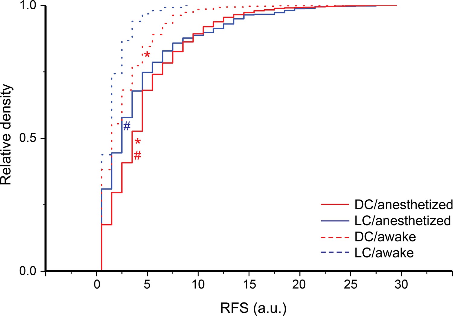
The receptive field sum (RFS) of dorsal cortex (DC) and lateral cortex (LC) neurons at different experimental preparations.
The cumulative distribution function of the RFS of all cells collected from DC or LC under different experimental preparations; Kruskal-Wallis ANOVA, χ2=346.9, p<0.001, post hoc Dunn’s test; *(DC vs LC): z=–6.4 and –4.47 with p<0.001 and 4.6×10⁻⁵ under anesthesia and awake preparations, respectively; #(anesthesia vs awake): z=13.6 and 7.8 with p<0.001 for DC and LC, respectively; mean ± SEM = 5.1 ± 0.08, 4.5 ± 0.2, 3.07 ± 0.1, and 2.0 ± 0.08 for (DC/anesthesia, median = 4, 2487 cells/4 animals), (LC/anesthesia, median = 3, 472 cells/7 animals), (DC/awake, median = 2, 647 cells/3 animals), (LC/awake, median = 2, 249 cells/3 animals).
Figure 11 with 1 supplement
The somatosensory responses from LC(microprism) in awake animals.
(A, C, E) The pseudocolor images show the auditory (white circles) or somatosensory (blue circles) responsive cells of the LC(microprism) as well as the merged response (green circles), respectively. (B, D) The pseudocolor images show onset (ON) (blue circles), offset (OFF) (green circles), or onset/offset (ON/OFF) (white circles) responsive cells of the LC(microprism) to auditory and somatosensory stimuli, respectively. (F) The pseudocolor images show enhanced (white circles) and suppressive response (blue circles) of the auditory responsive cells of the LC(microprism) following the bimodal stimulation based on their response index (RI). (G) A bar graph showing the percentage of responsive cells to auditory stimulation only or auditory selective cells (Aud-sel, yellow bars), to somatosensory stimulation only or somatosensory selective cells (Som-sel, blue bars), or nonselectively to both auditory and somatosensory stimulations (Aud/Som-nonsel, black bars) in modules vs matrix (chi-square test, χ2=42.5, p=4.4 × 10⁻⁸, % of responsive cells = 49%, 29%, and 22% for Aud-sel, Som-sel, and Aud/Som-nonsel [modules, 55 cells] and 89%, 3%, and 8% for Aud-sel, Som-sel, and Aud/Som-nonsel [matrix, 147 cells] – 3 animals, **p<0.05 vs modules). (H) A bar graph showing the percentage of all cells having auditory responses (Aud. resp) or those having somatosensory responses (Som. resp) in modules vs matrix (chi-square test, χ2=30.2, p=1.2 × 10⁻⁶, % of responsive cells [modules vs matrix]=21% vs 79% for [Aud-resp, 182 cells], 64% vs 36% for [Som-resp, 44 cells] – 3 animals, **p<0.05 vs modules). (I) A bar graph showing the percentage of auditory responsive cells with onset (Aud-ON) vs those with offset (Aud-OFF) responses in modules vs matrix (chi-square test, χ2=2.8, p=0.41, % of responsive cells [modules vs matrix]=21% vs 79% for [Aud-ON, 176 cells], 50% vs 50% for [Aud-OFF, 6 cells] – 3 animals, **p<0.05 vs modules). (J) A bar graph showing the percentage of auditory responsive cells with suppressed vs those with enhanced responses following bimodal stimulation in modules vs matrix (chi-square test = 31.9, p=5.2 × 10⁻⁷, matrix: the percentage of responding cells = 95% vs 5% for suppressed vs enhanced [modules, 40 cells] and 70% vs 30% for suppressed vs enhanced [matrix, 142 cells] – 3 animals, **p<0.05 vs modules). D: dorsal, R: rostral.
Figure 11—figure supplement 1
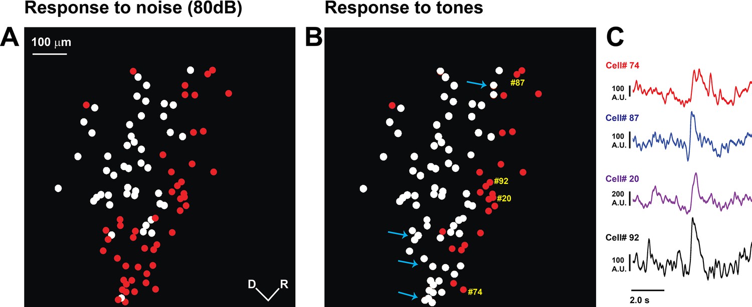
The activity of the nonresponsive cells of the LC(microprism) in awake animals.
(A) The pseudocolor image shows the nonresponsive (red circles) vs responsive (white circles) cells to the auditory stimulation with unmodulated broadband noise at the LC(microprism). (B) The pseudocolor image shows the nonresponsive (red circles) vs responsive (white circles) cells to the auditory stimulation with unmodulated broadband noise or pure tones (blue arrows) at the LC(microprism). (C) Time traces of the spontaneous activity of four nonresponsive cells (yellow numbers in B).
Tables
Key resources table
| Reagent type (species) or resource | Designation | Source or reference | Identifiers | Additional information |
|---|---|---|---|---|
| Strain, strain background (Mus musculus) | GAD67-GFP (GAD1GFP) | Generously given | N/A | Developed and shared with permission from Dr. Yuchio Yanagawa at Gunma University and obtained from Dr. Douglas Oliver at the University of Connecticut |
| Strain, strain background (Mus musculus) | Tg(Thy1-jRGECO1a)GP8.20Dkim/J | Jackson Laboratory, USA | 30525 | |
| Sequence-based reagent | jRGECO1a – primer | Transnetyx, USA | mApple-1 Tg | |
| Antibody | NeuN (D4G40) XP Rabbit mAB | Cell Signaling, USA | 62994 | (1:100) |
| Antibody | Goat anti-rabbit IgG conjugated to Alexa Fluor 405 | Thermo Fisher, USA | A-31556 | (1:200) |
Additional files
Download links
A two-part list of links to download the article, or parts of the article, in various formats.
Downloads (link to download the article as PDF)
Open citations (links to open the citations from this article in various online reference manager services)
Cite this article (links to download the citations from this article in formats compatible with various reference manager tools)
Microprism-based two-photon imaging of the mouse inferior colliculus reveals novel organizational principles of the auditory midbrain
eLife 12:RP93063.
https://doi.org/10.7554/eLife.93063.4


