A statistical framework for analysis of trial-level temporal dynamics in fiber photometry experiments
- Machine Learning Core, National Institute of Mental Health, United States
- Division of Biostatistics and Health Data Science, University of Minnesota, United States
- Laboratory for Integrative Neuroscience, National Institute on Alcohol Abuse and Alcoholism, United States
Figures
Figure 1
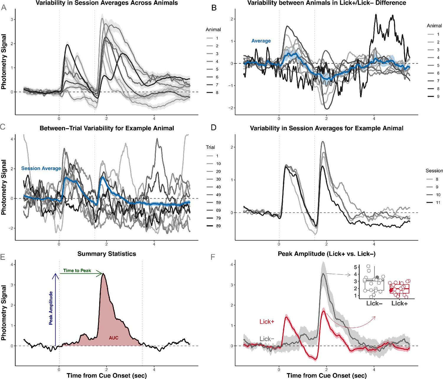
Variability in photometry signals highlights the need for trial-level analyses.
Signals were recorded from a Pavlovian task in which reward-delivery (sweetened water) followed a stimulus-presentation (0.5 sec auditory cue) after a 1 sec delay. Signals are aligned to cue-onset. (A) Signals exhibit heterogeneity across animals. Each trace is a trial-averaged signal on one session for one animal. (B) Signals exhibit heterogeneity across animals in the effect of condition. Each trace is from one animal on the same session as in (A). Signals were separately averaged across trials in which animals did (Lick+) or did not (Lick-) engage in anticipatory licking. Each trace represents the pointwise difference between average Lick+ and Lick- signals. (C) Signals exhibit heterogeneity across trials within animal. Each trace is a randomly selected trial from the same animal in the same session. (D) Signals exhibit heterogeneity across sessions. Each trace plotted is the trial-averaged signal for one session for one subject. (E) Illustration of common summary measures. Depending on the authors, Area-Under-the-Curve (AUC) can be the area of the shaded region or the average signal amplitude. (F) Example hypothesis test of Lick+/Lick- differences using peak amplitude as the summary measure. All signals are measurements of calcium dynamics from axons of mesolimbic dopamine neurons recorded from fibers in the nucleus accumbens (Coddington et al., 2023).
Figure 2
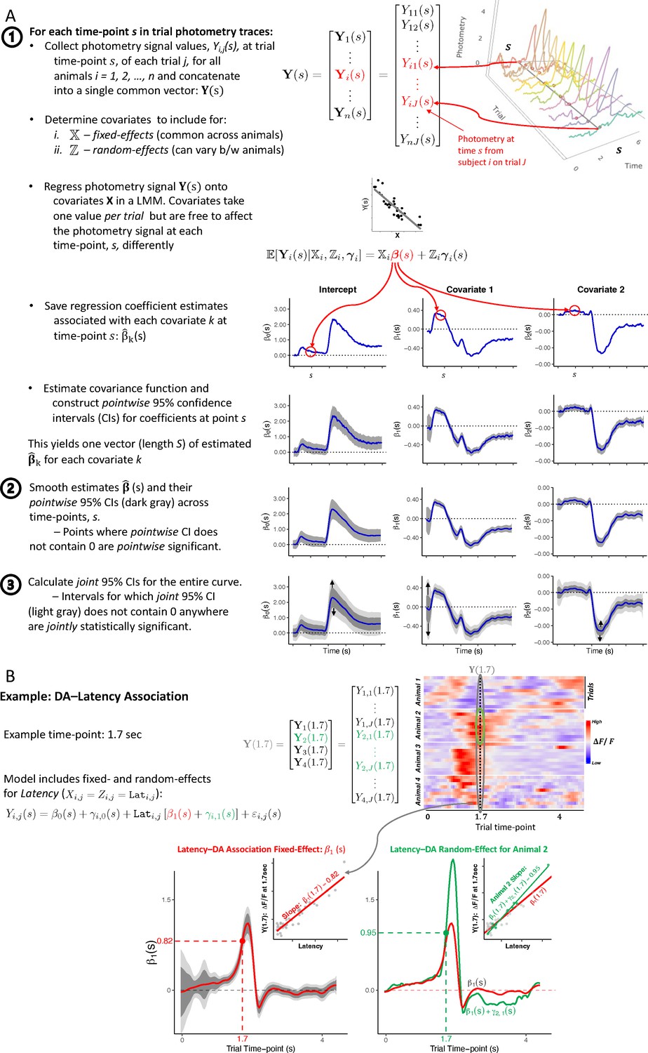
Functional Linear Mixed Models estimation.
(A) General procedure. (B) Example analysis of Latency-signal (Latency-to-lick) association. To illustrate how the plots are constructed, we show the procedure at an example trial time-point ( sec), corresponding to values in the heatmap [Top right]. Each point in the FLMM coefficient plot [Bottom Left] can be conceptualized as pooling signal values at time across trials/animals (a slice of the heatmap) and correlating that pooled vector, , against Latency, via a linear mixed model (LMM). [Bottom Right] shows how functional random-effects can be used to model variability in the Latency-dopamine (DA) slope across animals. The inset shows how at , the model treats an example animal’s slope (green), , to differ from the shared/common fixed-effect (red), .
Figure 3
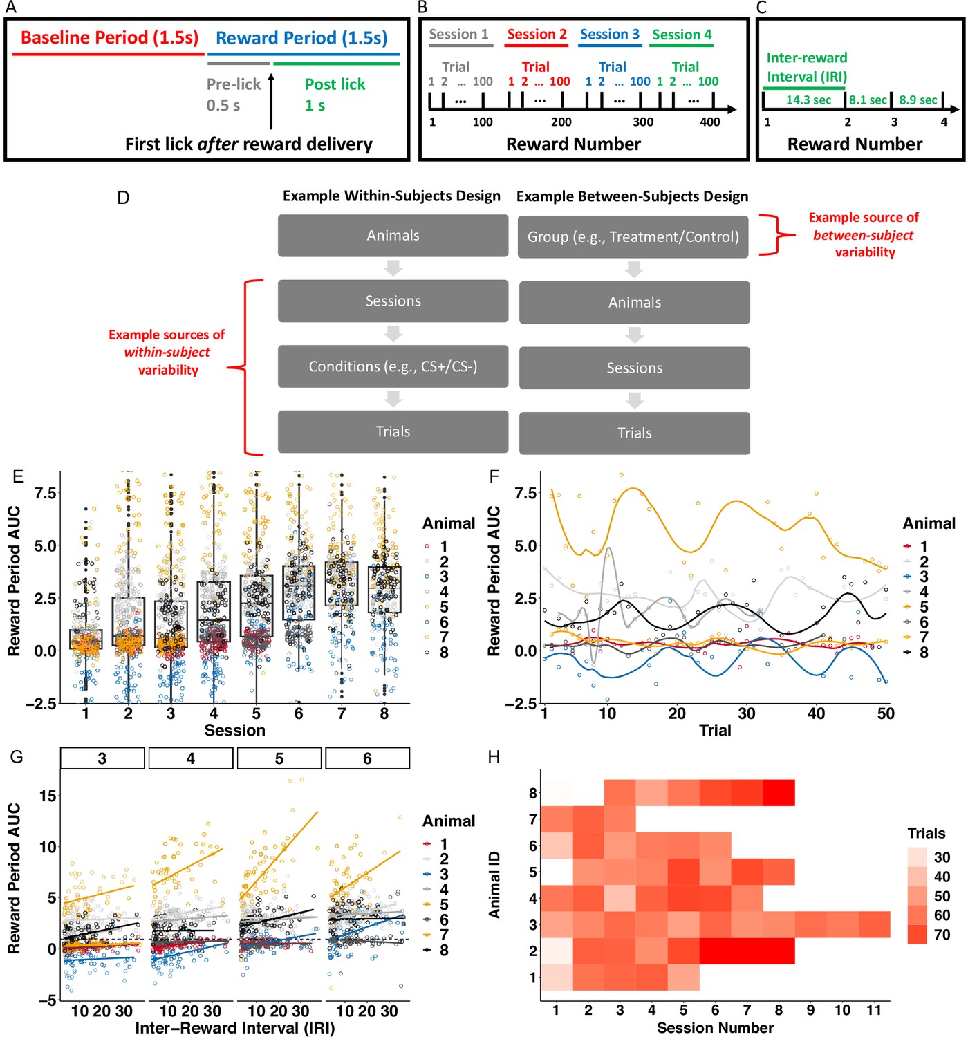
Nested longitudinal designs in photometry experiments can result in correlation patterns and missing data that dilute effects if not unaccounted for statistically.
Descriptive statistics and figures pertain to data from Jeong et al., 2022, reanalyzed in section Using FLMM to test associations between signal and covariates throughout the trial. (A) Experiment trial time-windows used to construct photometry signal summary measures (Area Under the Curve, AUC). The reward was delivered at random times and signals were aligned to the first lick following reward delivery. Reward delivery may occur during the Baseline Period or Reward Period, depending on the lick time. (B) The Reward Number is defined as the cumulative number of rewards (interchangeably referred to as ‘trials’) pooled across sessions. Each session involved the delivery of 100 trials. (C) The time between two rewards (inter-reward interval or IRI) was a random draw from an exponential distribution (mean 14). (D) Examples of experimental designs that exhibit hierarchical nesting structure. Trials/sessions and conditions such as cue-type (e.g. CS+/CS-) contribute to variability within-animal. Between-subject variability can arise from, for example, experimental groups, photometry probe placement, or natural between-animal differences. (E) Reward Period AUC values are correlated across sessions. Each dot indicates the average reward period AUC value of one trial. Between-session correlation in AUC values can be seen within-subject since reward period AUC values are similar within-animal on adjacent sessions. Between-session correlation can be seen on average across animals: session boxplot medians are similar in adjacent sessions. (F) Temporal correlation within-subject on session 3, chosen because it is the only session common to all animals. Reward period AUC on each trial for any animal is similar on adjacent trials. (G) Lines show association (ordinary least square, OLS) between IRI and reward period AUC for each animal and session, revealing individual differences in association magnitude. The heterogeneity in line slopes highlights the need for random-effects to account for between-animal and between-session variability. (H) Number of sessions and trials per session (that meet inclusion criteria) included varies considerably between animals. For example, one animal’s data was collected in sessions 1–11 while another’s was collected in sessions 1–3.
Figure 4
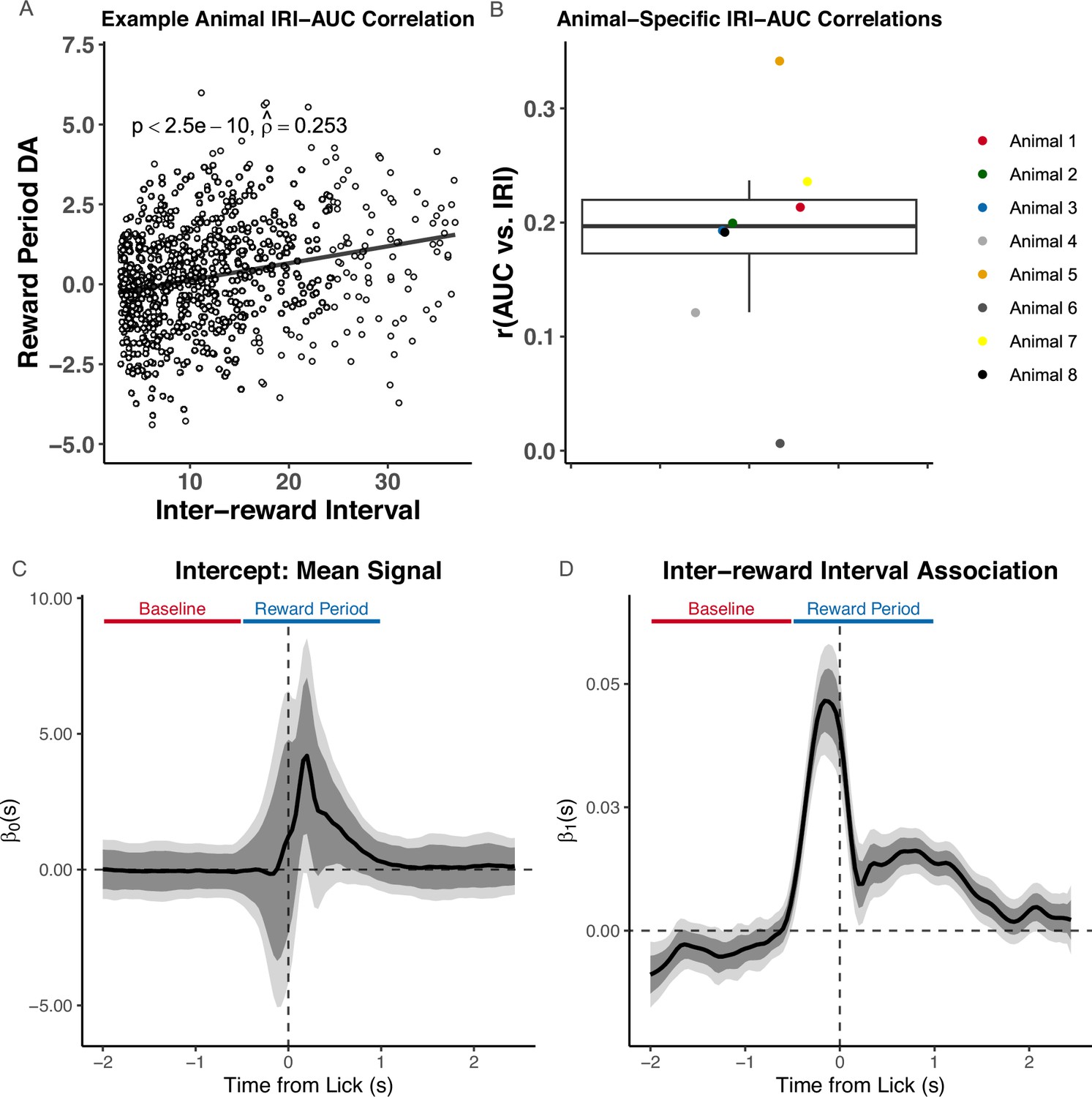
Functional Linear Mixed Models (FLMM) reveals distinct components obscured by summary measure analyses.
(A, B) show a recreation of statistical analyses conducted by Jeong et al., 2022 on the random inter-trial interval (IRI) reward delivery experiment, and (C, D) show our analyses. (A) Analysis of IRI–Area Under the Curve (AUC) correlation on all trials in an example animal, as presented in Jeong et al., 2022. (B) Recreation of boxplot summarizing IRI–AUC correlation coefficients from each animal. (C,D) Coefficient estimates from FLMM analysis of IRI–dopamine (DA) association: functional intercept estimate (C), and functional IRI slope (D). Although we do not use AUC in this analysis, we indicate the trial periods, ‘Baseline’ and ‘Reward Period’, that Jeong et al., 2022 used to calculate the AUC. They quantified DA by a measure of normalized AUC of during a window ranging from 0.5 sec before to 1 sec after the first lick following reward delivery. All plots are aligned to this first lick after reward delivery. The IRI–DA association is statistically significantly positive in the time interval ∼[–0.5, 1.75] sec.
Figure 5
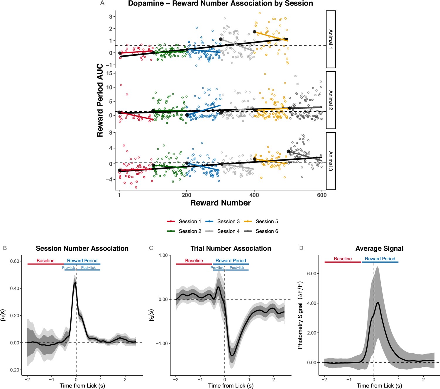
Functional Linear Mixed Models (FLMM) identifies within-session signal decreases obscured by standard analyses.
(A) Visualization of the Simpson’s paradox: the Area Under the Curve (AUC) decreases within-session, but increases across sessions. Plot shows Reward Number–AUC linear regressions fit to data pooled across sessions (black lines), or fit to each session separately (colored lines) in three example animals. Each colored dot is the AUC value for that animal on the corresponding session and trial. The black dots at the left of each color line indicate the intercept value of the session- and animal-specific linear regression model. Intercepts were parameterized to yield the interpretation as the 'expected AUC value on the first trial of the session for that animal.' The dotted lines indicate the animal-specific median of the intercepts (across sessions) and are included to visualize that the intercepts increase over sessions. (B, C) Coefficient estimates from FLMM analysis of the Reward Number–dopamine (DA) association that models Reward Number with Session Number and Trial Number (linear) effects to capture between-session and within-session effects, respectively. The plots are aligned to the first lick after reward-delivery. The Baseline and Reward Period show the time-windows used to construct AUCs in the summary measure analysis from Jeong et al., 2022. Pre-lick and post-lick time-windows indicate the portions of the Reward Period that occur before and after the lick, respectively. The Session Number effect is jointly significantly positive roughly in the interval [–0.25,0.5] sec, and peaks before lick-onset. This suggests DA increases across sessions during that interval. The Trial Number effect is briefly pointwise significantly positive around ∼−0.3 sec and jointly significantly negative in the interval [0, 2.5] sec. This suggests DA decreases across trials within-session during the interval [0, 2.5] sec. (D) Average signal pooled across sessions and animals. Shaded region shows standard error of the mean.
Figure 6
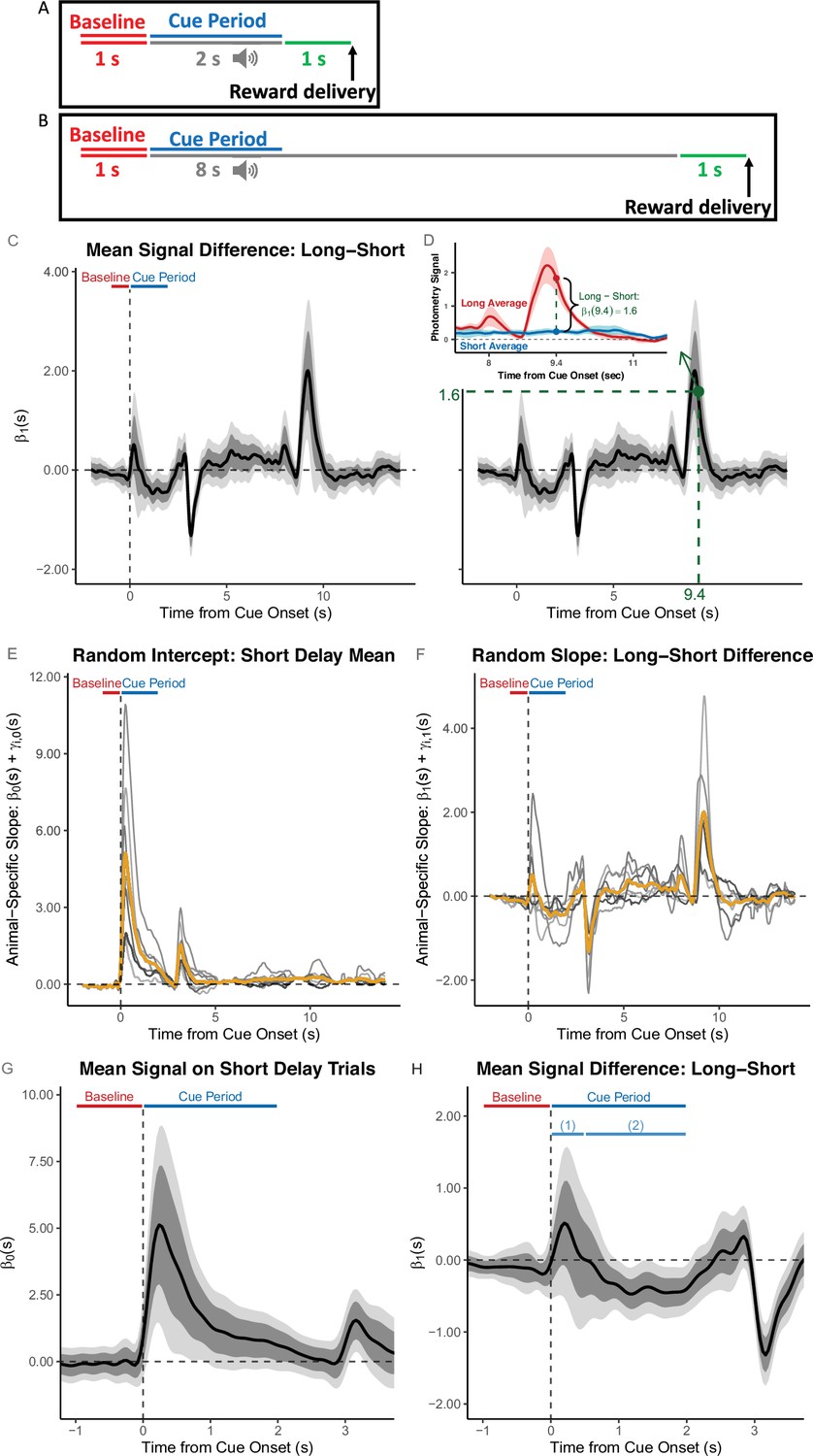
Functional Linear Mixed Models (FLMM) identifies significant temporal dynamics effects missed by summary measure analyses.
The analysis of the Delay Length change experiment by Jeong et al., 2022 used the following summary measure: the average Cue Period AUC − Baseline AUC (Area Under the Curves, AUCs in the windows [0,2] and [–1,0] sec, respectively, relative to cue onset). (A, B) Behavioral task design and Baseline/Cue Period are illustrated for short-delay (A) and long-delay (B) sessions. (C-H) These plots show coefficient estimates from FLMM re-analysis of the experiment. (C) The coefficient value at time-point on the plot is interpreted as the mean change in average dopamine (DA) signal at time-point between long- and short-delay trials (i.e. positive values indicate a larger signal on long-delay trials), aligned to cue onset. (D) Same Figure as in (C) but the inset shows the interpretation of an example time-point (): the difference in magnitude between the average traces (pooled across animals and trials) of long- and short- delay sessions. (E, F) Gold lines indicate the fixed-effect estimates and gray lines indicate animal-specific estimates (calculated as the sum of functional fixed-effect and random-effect estimates (Best Linear Unbiased Predictor)) for the random intercept, and random slope, respectively. (G, H) Fixed-effect coefficient estimates shown with expanded time axis. In (H), it is clear that long-delay trials exhibit average (relative) increases (sub-interval (1)) and decreases (sub-interval (2)) in the signal that would likely cancel out and dilute the effect, if analyzing with a summary measure (AUC) that averages the signal over the entire Cue Period.
Figure 7
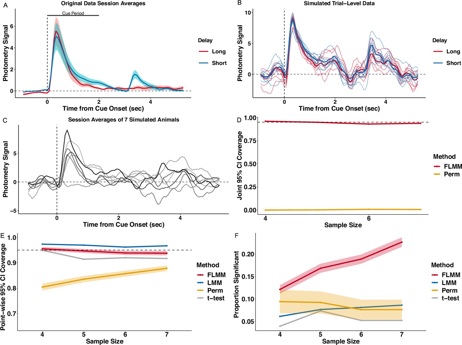
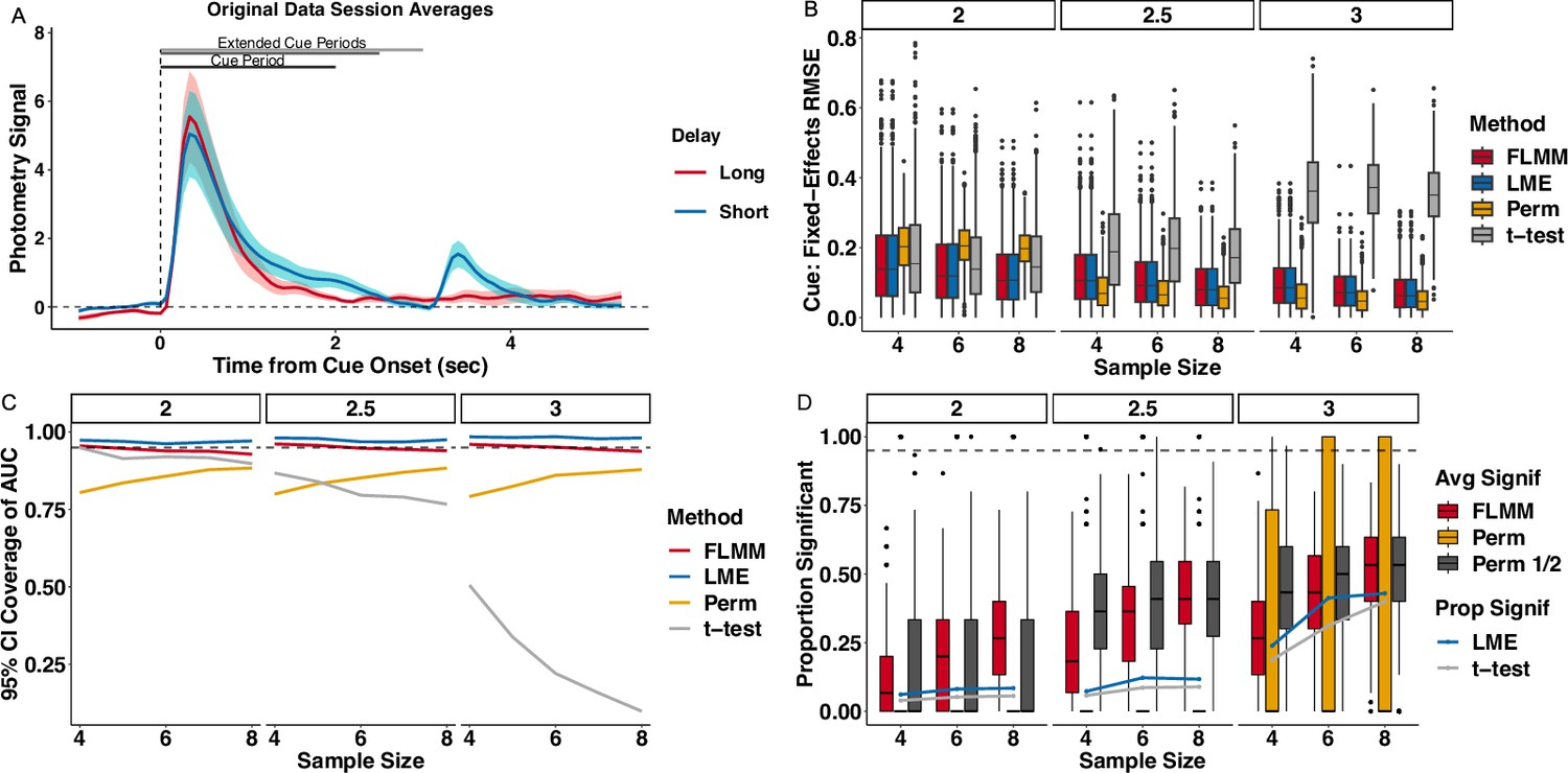
Realistic simulation experiments show that Functional Linear Mixed Models (FLMM) exhibits desirable statistical properties for photometry analyses.
The simulation produces synthetic photometry data similar to Jeong et al., 2022, with the same sources of variability across trials and animals. (A) Lines show average traces from the original photometry data. The traces are averaged across trials and animals from the last short- and the first long-delay session. The bar shows the cue period analyzed in the paper and in our experiments. (B) Each thin line is the signal from a single simulated trial from the same ‘animal’; bold lines show the average trace for each trial type. (C) Each line is the trial-averaged trace from one session for seven simulated ‘animals.’ (D) FLMM exhibits approximately correct joint 95% confidence interval (CI) coverage. Perm does not provide joint CIs and thus its joint coverage is low, as expected. (E) FLMM exhibits approximately correct pointwise 95% CI coverage. (F) FLMM improves statistical power during the cue period compared to standard methods at each sample size tested. Power is calculated for Perm based on the full consecutive threshold criteria. For figures (E) and (F) the linear mixed models (LMM) and t-test were fit on the cue period Area Under the Curve (AUC) and thus each replicate yields one indicator of CI inclusion and statistical significance. We represent the corresponding proportions with a line plot. For other methods, estimates are provided at each time-point. We therefore average performance across the cue period and then summarize the variability of these replicate-specific averages with a 95% confidence band.
Figure 8
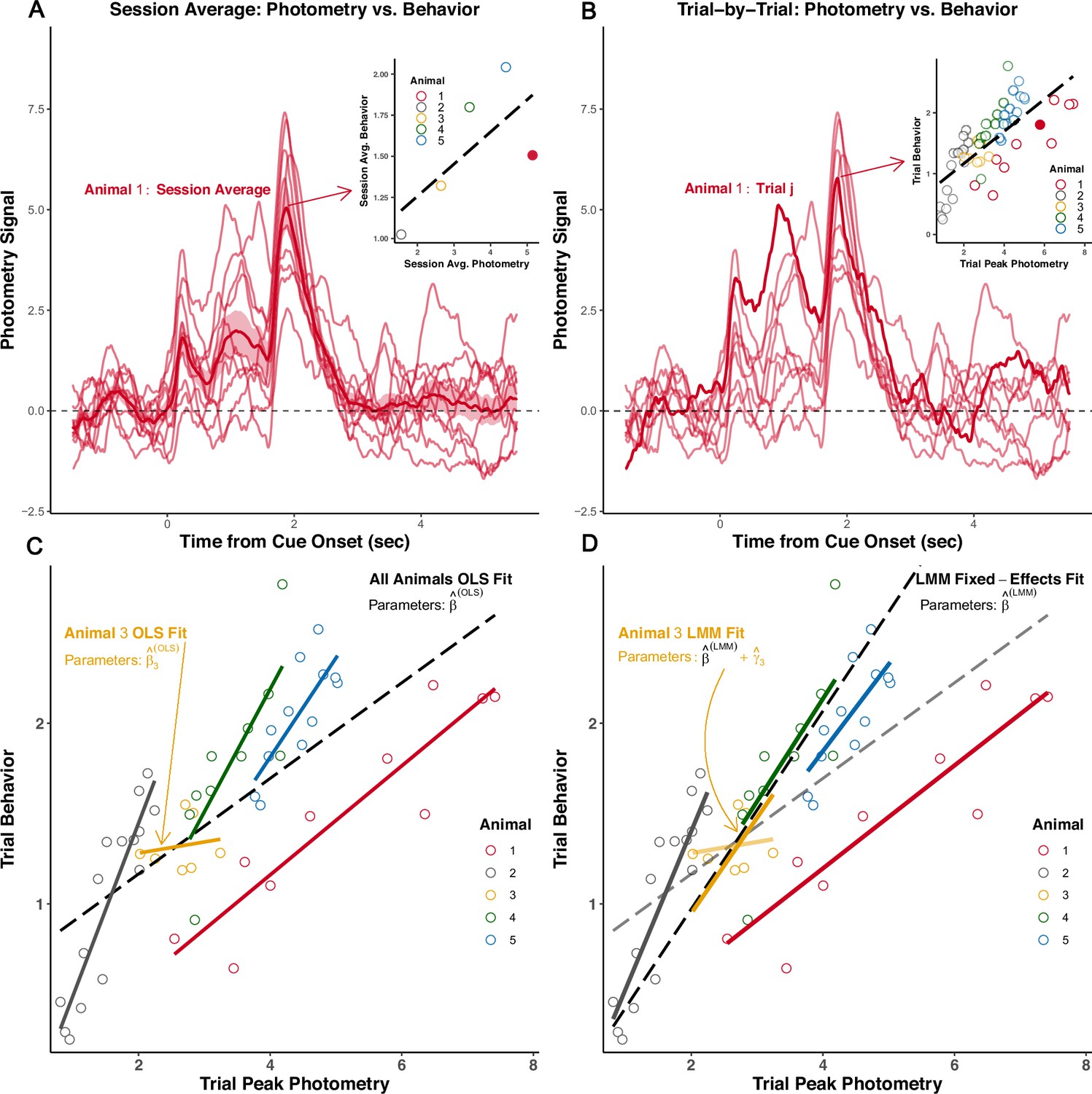
Example repeated measures data from a single test session.
(A) Session-average approach: photometry signals from all trials for Animal 1 are averaged across trials and summarized (peak amplitude). The session-average summary is then plotted (inset) against the session-average behavior for each of five animals. Example animal’s session average is the filled circle. (B) Trial-level approach: the trial-level signal summary measure (peak amplitude) is pooled across animals and correlated with trial-level behavior. An example signal from one trial for Animal 1 is highlighted in the trace plot. That example trial is represented as the filled circle in the inset. Each dot in the inset is one trial from one animal; dot color indicates the animal ID. (C) Inset from (B) is magnified. Linear regressions (OLS: Ordinary least squares) fit separately to each animal’s trial-level data. A global regression fit to the trial-level data pooled across animals is displayed as the dotted black line. (D) Linear mixed modeling (LMM) strikes a balance between one model common to all animals and fitting many animal-specific models. The ‘global’ fixed-effects fit (from ) and the fits including the subject-level random-effect estimates (Best Linear Unbiased Predictor) are displayed. Subject-specific fit for animal is calculated from: . Note the fixed-effects, , and random-effects, , are estimated in the same model.
Appendix 1—figure 1
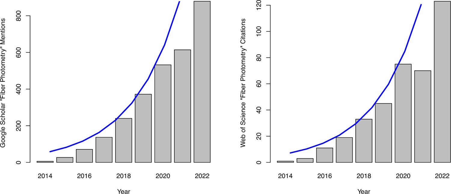
Photometry citations by year.
[Left] Google scholar mentions of the string ‘Fiber Photometry’ by year. There were 549 mentions between January 1, 2023 and June 22, 2023. [Right] Web of Science citations of papers that include the string ‘Fiber Photometry’ by year. There were 50 citations between January 1, 2023 and June 22, 2023. Blue lines indicate fitted values from an exponential fit to the data: , where and were estimated with the nls package in R. The 1500 references to photometry described in the main text refers to Google Scholar mentions in the 12 months prior to June 2023.
Appendix 4—figure 1
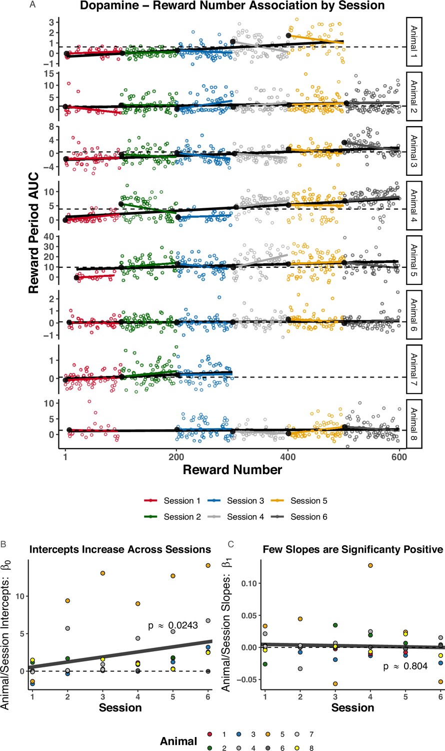
Reward Number–Area Under the Curve (AUC) correlation within-session and across-session.
(A) Color indicates session number, rows denote animal number. Trial Number is the within-session Reward Number and ranges from 1 to 100 for each session. The black line that spans across sessions is a Reward Number–AUC linear regression fit, while the session color lines indicate a within-session Trial Number–AUC linear regression fit. The large black circles on the left side of each session-specific fit is the intercept, paramterized to yield the interpretation as the ‘expected AUC on the first trial of the corresponding session.’ Dotted horizontal lines are set at the median of the intercepts to facilitate comparison. The intercepts tend to rise across sessions, while few slopes are significantly positive. (B, C) Each dot indicates the estimated intercept value (B) or slope (C) from the fits shown in (A). Lines and p-values were calculated in an linear mixed model (LMM) that was fit to the session-specific linear regression slopes, , and intercepts, , shown in (A). The LMM included animal-specific random intercepts and slopes. These plots quantify the trend observed in (A): the estimated intercepts significantly increase across sessions, but the slopes are mostly negative.
Appendix 4—figure 2
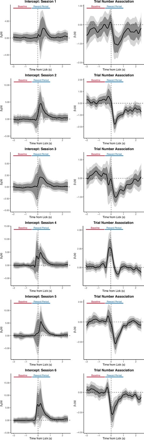
Trial Number–dopamine (DA) correlation within-session on the random inter-reward interval (IRI) task.
Row indicates session number. The intercept is paramterized to yield the interpretation as the ‘expected signal magnitude on the first trial of the corresponding session.’ Effects are aligned to the first lick after reward delivery. This is the session-by-session version of the analysis presented in Figure 5J–K.
Appendix 4—figure 3
Functional Linear Mixed Models (FLMM) reveals details occluded by summary measure analyses.
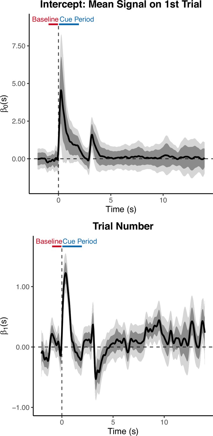
Coefficient estimates from an FLMM analysis of the random inter-trial interval (IRI) reward delivery experiment. The top row contains the intercept term plots where the title provides an interpretation of the intercept: the average dopamine (DA) signal on trials when Lick Rate is at its average value. The bottom row shows the coefficient estimate plot of the covariate in the model. The ‘Baseline’ and ‘Reward Period’ bars show the trial period that the original authors used to calculate the summary measure (Area Under the Curve, AUC). Specifically, they quantified DA by a measure of normalized AUC of during a window 0.5 sec before to 1 sec after the first lick following reward delivery. All plots are aligned to this first lick after reward delivery. The interpretation of the y-value of the bottom plot at any time-point : the mean change in the dopamine signal at for a one unit change in Lick Rate. Association between DA and Lick Rate aligned to lick bout onset. Time-points when Lick Rate was negatively associated with DA (negative coefficient estimates in the final 1 sec of the 1.5 sec window) may have diluted time-points when they were positively associated (positive coefficient estimates in the first 0.5 sec of the reward period).
Appendix 4—figure 4

Random inter-reward interval (IRI) experiment aligned to Lick-onset: Reward Number–dopamine (DA) association analyzed as within-session (Trial Number) and between-session (Session Number) linear effects.
The average reward signal shows the average trace with standard error of the mean indicated by the shaded region. The Trial Number Session Number effects are functional linear mixed model (FLMM) coefficient estimate plots.
Appendix 4—figure 5
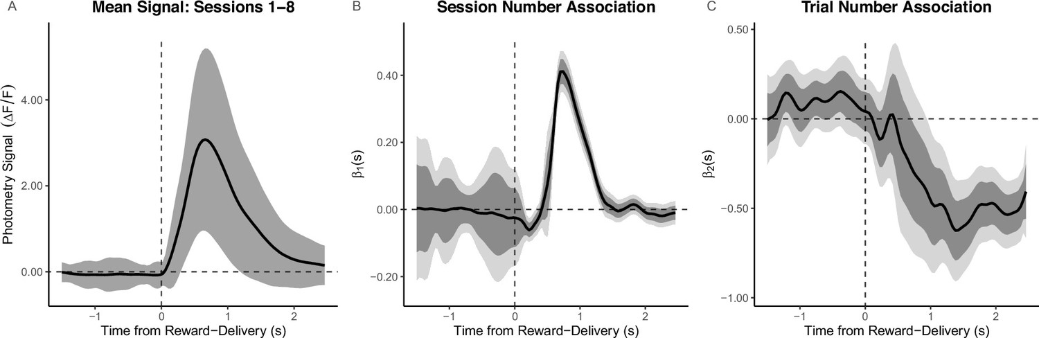
Random inter-reward interval (IRI) experiment aligned to reward-delivery: Reward Number–dopamine (DA) association analyzed as within-session (Trial Number) and between-session (Session Number) linear effects.
The average reward signal shows the average trace with standard error of the mean indicated by the shaded region. The Trial Number Session Number effects are functional linear mixed model (FLMM) coefficient estimate plots.
Appendix 4—figure 6
Functional Linear Mixed Models (FLMM) identifies how the signal increases across trials during the Cue Period and decreases across trials after reward-delivery (3 sec).
Appendix 4—figure 7

Background reward experiment analyses.
Appendix 4—figure 8
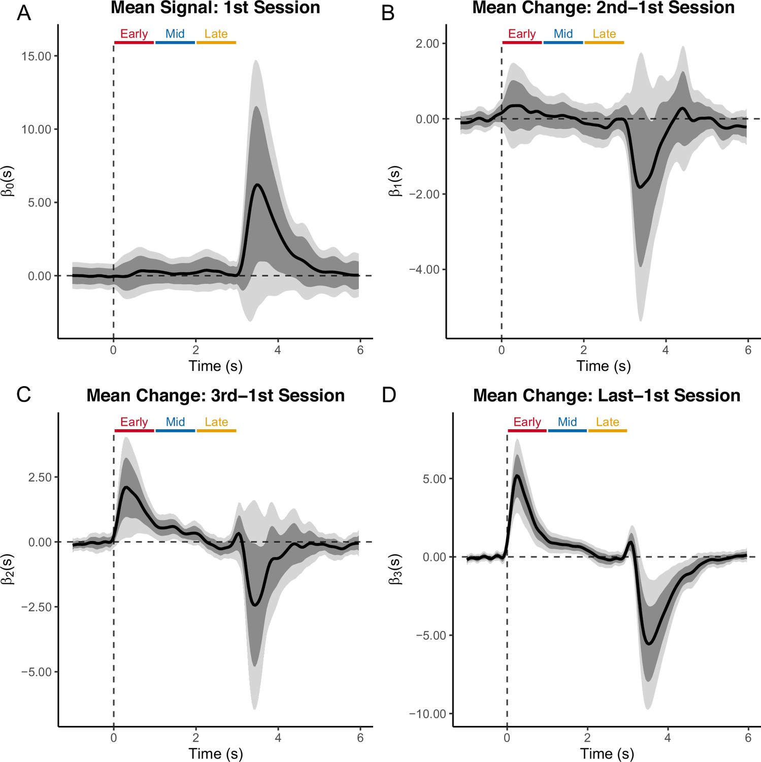
Functional Linear Mixed Models (FLMM) identifies how the signal evolves across trial time-points, and how the temporal location of transients progresses across sessions in a statistically significant manner.
The panels show coefficient estimates from FLMM analyses of the ‘backpropagation’ experiment. Panel (A) contains the intercept term plot corresponding to the average signal on the first session of training. The ‘Early’ (0–1 sec), ‘Mid’ (1–2 sec), and ‘Late’ (2–3 sec) bars show the trial time-periods that the original authors used to calculate summary Area Under the Curve (AUC) measures. Trials are aligned to cue onset (cues lasted 2 sec) and rewards were delivered at 3 sec. Panels (B-D) show the coefficient estimates corresponding to the mean change in signal values from the second, third, or, fourth sessions, respectively, compared to the first session (positive values indicate an increase from the first session). Plots are aligned to cue onset.
Appendix 4—figure 9
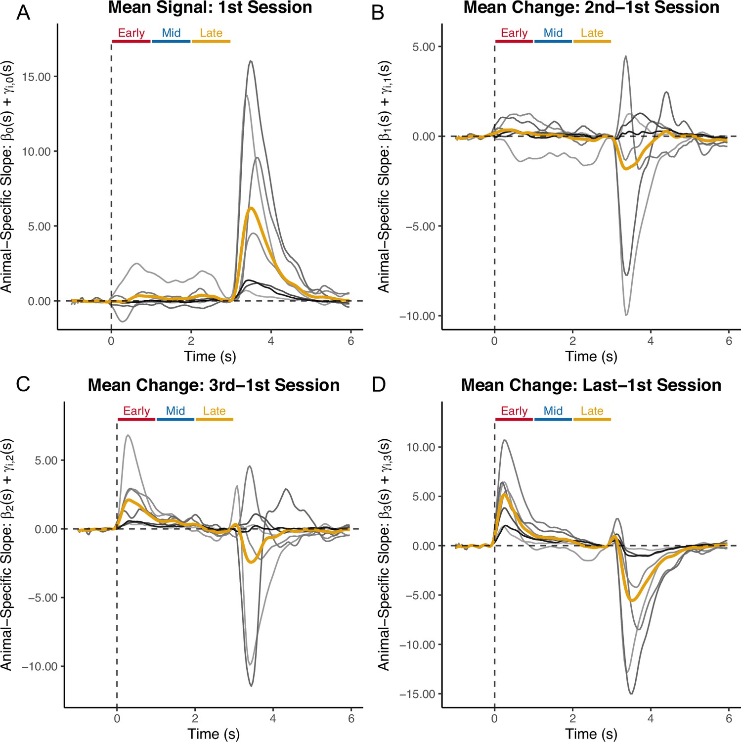
Individual-level coefficient estimates from functional linear mixed model (FLMM) analyses of the ‘backpropagation’ experiment: gold lines indicate the fixed-effect estimates and gray lines indicate animal-specific functional random-effect estimates (Best Linear Unbiased Predictor).
Panel (A) contains the intercept term plot where the title provides an interpretation: the average signal on the first session of training. The ‘Early’ (0–1 sec), ‘Mid’ (1–2 sec), and ‘Late’' (2–3 sec) bars show the trial time-periods that the original authors used to calculate summary Area Under the Curve (AUC) measures. Trials are aligned to cue onset and rewards were delivered at 3 sec. Panels (B-D) show the coefficient estimates which are interpreted as the change in mean signal from the second, third, or fourth sessions, respectively, compared to the first session (positive values indicate an increase from the first session). Plots are aligned to cue onset.
Appendix 5—figure 1
Summary measure analyses are highly sensitive to minor changes in the summary time-window.
(A) Average short/long-delay data. Bars show cue period length used in (2 sec) and ‘extended‘ delays analyzed in additional simulations. (B) Estimation error (RMSE), where , associated with a mean difference during the cue periods (panels) and on the x-axis. Lower numbers indicate more accurate estimates. (C) pointwise 95% CI coverage is associated with a mean difference during cue period (panels) and on the x-axis. Higher values indicate better CI coverage. (D) Statistical power during cue period. The linear mixed model (LMM) and t-test were fit on the signal averaged over the cue period and thus each simulation replicate yields a single indicator of CI inclusion or statistical significance, which we represent with a line plot. For other methods, estimates are provided at each time-point, and performance is averaged across the time-points. We summarize these simulation replicate-specific averages with a boxplot.
Appendix 5—figure 2

Statistical power associated with mean difference defining the cue period as 2 sec, 2.5 sec, and 3 sec (panels) and sample sizes (numbers of animals) on the x-axis.
The two panels presents the same data in either violin or boxplot forms. Higher numbers indicate better power. For functional linear mixed model (FLMM) and Perm, power is averaged across the time-points in the cue period whereas the others assess the power using the average signal (across the cue period) as the outcome. Since each simulation replicate takes the proportion of significant time-points in the cue period for FLMM and Perm, these are presented as boxplots (or violin plots), whereas the rest are simply presented as the proportion of simulation replicates that identified the mean signal during the cue as statistically significant (either 0 or 1 for each replicate).
Appendix 5—figure 3

Time to fit functional linear mixed model (FLMM) fit with our software (using a closed-form variance calculation) on simulated data (each data point represents one replicate).
pffr shows the time to fit the functional linear mixed model (with the same model specification) with the pffr() function in the refund package. Number of animals in simulations shown in plots ranges from 4 to 8 (i.e. ).
Appendix 5—figure 4
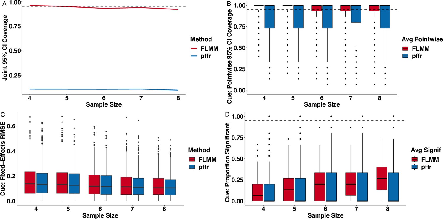
Functional Linear Mixed Models (FLMM) fit with our software achieves comparable or superior performance to the functional linear mixed model (with the same model specification) fit with the pffr() function in the refund package.
(A) FLMM achieves joint 95% CI coverage at roughly the nominal level. pffr does not provide joint 95% CIs and thus the pointwise 95% CIs that it does provide achieve low joint coverage. (B) FLMM achieves pointwise 95% CI coverage at or above the nominal level. The pointwise 95% CI coverage of pffr is close to but below the nominal level. pointwise 95% CI coverage associated with mean difference during cue period (panels) and on the x-axis. Higher values indicate better CI coverage. (C) FLMM and pffr exhibit comparable fixed-effects estimation performance. Estimation error (RMSE), where , associated with mean difference during the cue periods (panels) and on the x-axis. Lower numbers indicate more accurate estimates. (D) FLMM exhibits superior statistical power compared to pffr during the cue period. (B-D) Since estimates are provided at each timepoint for both methods, pointwise performance is averaged across the time-points. We summarize these simulation replicate-specific averages as one point in a boxplot.
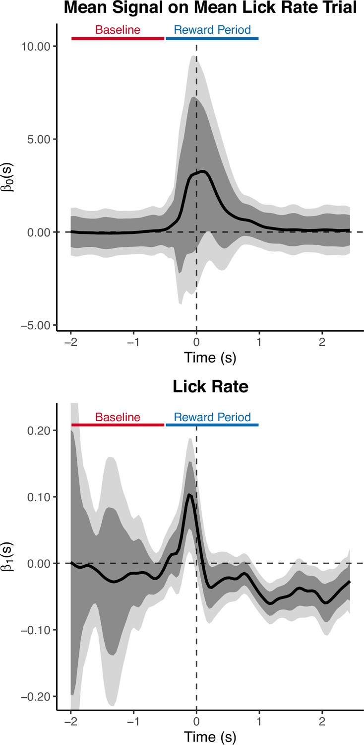
Appendix 6—figure 1
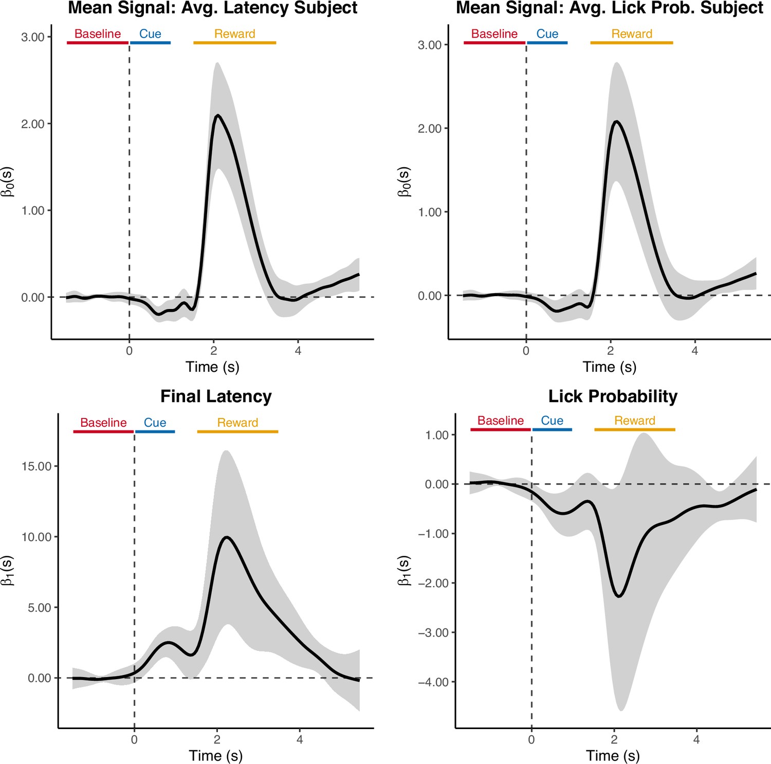
Coefficient estimates from Functional Linear Mixed Models (FLMM) analyses of Final Latency and Lick Probability models.
The top row contains intercept term plots where the title provides interpretation of the intercept: the average dopamine neuron calcium (NAc-DA) signal on trials when the covariates in the model are at their average value. The bottom row shows the coefficient estimate plot of the covariate in the model. (Left) Association between average NAc-DA (averaged over first 100 trials) and latency to lick Final Latency (averaged over trials 700–800). (Right) Association between average NAc-DA (averaged over first 100 trials) lick probability (averaged over trials 700–800).
Appendix 6—figure 2

Coefficient estimates from a single functional linear mixed model (FLMM) analysis of Final Latency × Lick State interaction model (including main effects).
A simple FLMM model enables characterization of how the association between photometry signals and behavioral responding (Final Latency) differs between conditions (Lick+/Lick-) at each time-point in the trial. Panel (A) contains the intercept term plot where the title provides an interpretation: the average photometry signal on Lick- trials for animals that exhibit average Final Latency values. Panels (B-D) show the three covariates of main effects and interaction of Lick State and Final Latency. The Final Latency functional coefficient is interpreted as the effect of Final Latency on Lick- trials. The Lick State main effect is interpreted as the difference in average NAc-DA between Lick+ and Lick- trials for an animal with an average Final Latency value. The interaction is interpreted as a difference in differences: during the Reward period, a 1 standard deviation increase in average Final Latency is associated with pointwise significantly higher NAc–DA signals on Lick+ than on Lick- trials (with a portion of joint significance) during most of the Reward period.
Tables
Appendix 2—table 1
Functional intercept .
Percentage of time-points in which the coefficient estimates are statistically significant. We compare the Benjamini–Hochberg (BH) correction applied to pointwise linear mixed models (LMM) models, the Functional Linear Mixed Models (FLMM) pointwise 95% CIs (Pointwise), and the FLMM joint 95% CIs (Joint). The proportion of points that are significant with the Benjamini–Hochberg (BH) approach jump around between 20-40Hz and then dramatically decrease as the sampling rate increases. In contrast, the FLMM Pointwise and Joint CIs are relatively stable and show only slight reductions in the proportion of points that are significant as the sampling rate increases.
| Sampling rate (Hz) | BH | Pointwise | Joint |
|---|---|---|---|
| 20 | 31.00 | 23.58 | 9.17 |
| 25 | 0.73 | 23.27 | 9.09 |
| 30 | 30.23 | 22.67 | 8.72 |
| 40 | 1.09 | 22.66 | 8.50 |
| 50 | 0.73 | 22.38 | 8.28 |
| 125 | 0.80 | 22.02 | 7.63 |
Appendix 2—table 2
Functional slope .
Percentage of time-points in which the coefficient estimates are statistically significant. We compare the Benjamini–Hochberg (BH) correction applied to pointwise linear mixed models (LMM) models, the Functional Linear Mixed Models (FLMM) pointwise 95% CIs (Pointwise), and the FLMM joint 95% CIs (Joint). The BH identifies no statistically significant effects at any time-points, whereas the the FLMM Pointwise and Joint CIs identify significant effects at a relatively consistent proportion of time-points.
| Sampling rate (Hz) | BH | Pointwise | Joint |
|---|---|---|---|
| 20 | 0 | 46.72 | 17.90 |
| 25 | 0 | 44.36 | 16.73 |
| 30 | 0 | 43.31 | 15.41 |
| 40 | 0 | 43.57 | 15.90 |
| 50 | 0 | 43.46 | 14.39 |
| 125 | 0 | 42.15 | 13.66 |
Appendix 3—table 1
Regression model classes based on functional vs scalar response variables and for longitudinal (repeated measures) vs cross-sectional data.
We use ‘functional mixed models’ as a short-hand for function-on-scalar mixed models. We use ‘functional regression’ as a short-hand for single-level function-on-scalar regression.
| Longitudinal | Cross-sectional | |
|---|---|---|
| Functional | Functional mixed models | Functional regression |
| Scalar | Generalized linear mixed-effects (GLMM) | Generalized linear models (GLM) |
Appendix 3—table 2
Cross-sectional regression model classes based on functional vs. scalar predictor variables (i.e. covariates) and functional vs. scalar outcome variables.
We take the FoFR, FoSR, and SoFR to be the single-level (non-longitudinal) versions of these methods.
| Functional outcome | Scalar outcome | |
|---|---|---|
| Functional predictors | Function-on-function regression (FoFR) | Scalar-onfunction regression (SoFR) |
| Scalar predictors | Function-onscalar regression (FoSR) | Generalized linear models (GLM) |
Additional files
Download links
A two-part list of links to download the article, or parts of the article, in various formats.
Downloads (link to download the article as PDF)
Open citations (links to open the citations from this article in various online reference manager services)
Cite this article (links to download the citations from this article in formats compatible with various reference manager tools)
A statistical framework for analysis of trial-level temporal dynamics in fiber photometry experiments
eLife 13:RP95802.
https://doi.org/10.7554/eLife.95802.3


