Volume electron microscopy reveals unique laminar synaptic characteristics in the human entorhinal cortex
- Laboratorio Cajal de Circuitos Corticales, Centro de Tecnología Biomédica, Universidad Politécnica de Madrid, Spain
- Instituto Cajal, Consejo Superior de Investigaciones Científicas (CSIC), Spain
- Centro de Investigación Biomédica en Red sobre Enfermedades Neurodegenerativas (CIBERNED), ISCIII, Spain
Figures
Figure 1 with 2 supplements
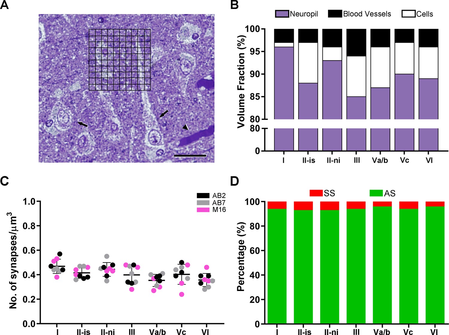
Microatatomical analyses of the medial entorhinal cortex (MEC).
(A) Semithin section, stained with toluidine blue, with a superimposed grid, where points hitting the different cortical elements were counted (grid spacing of 5 µm). Black arrowhead indicates a blood vessel; black arrows indicate cell bodies. (B) Graph showing the volume fraction of every cortical element. Values are detailed in Supplementary file 1a and b. (C) Mean synaptic density (± SD) per layer of the MEC. Each colored dot represents a stack of images from the analyzed cases AB2, AB7, and M16 (see Supplementary file 1p for details). No differences in the mean synaptic densities were found between layers (Kruskal–Wallis [KW]; p>0.05). (D) Proportion of asymmetric synapses (AS) and symmetric synapses (SS) per layer, expressed as percentages. Scale bar (in A): 25 µm.
Figure 1—figure supplement 1
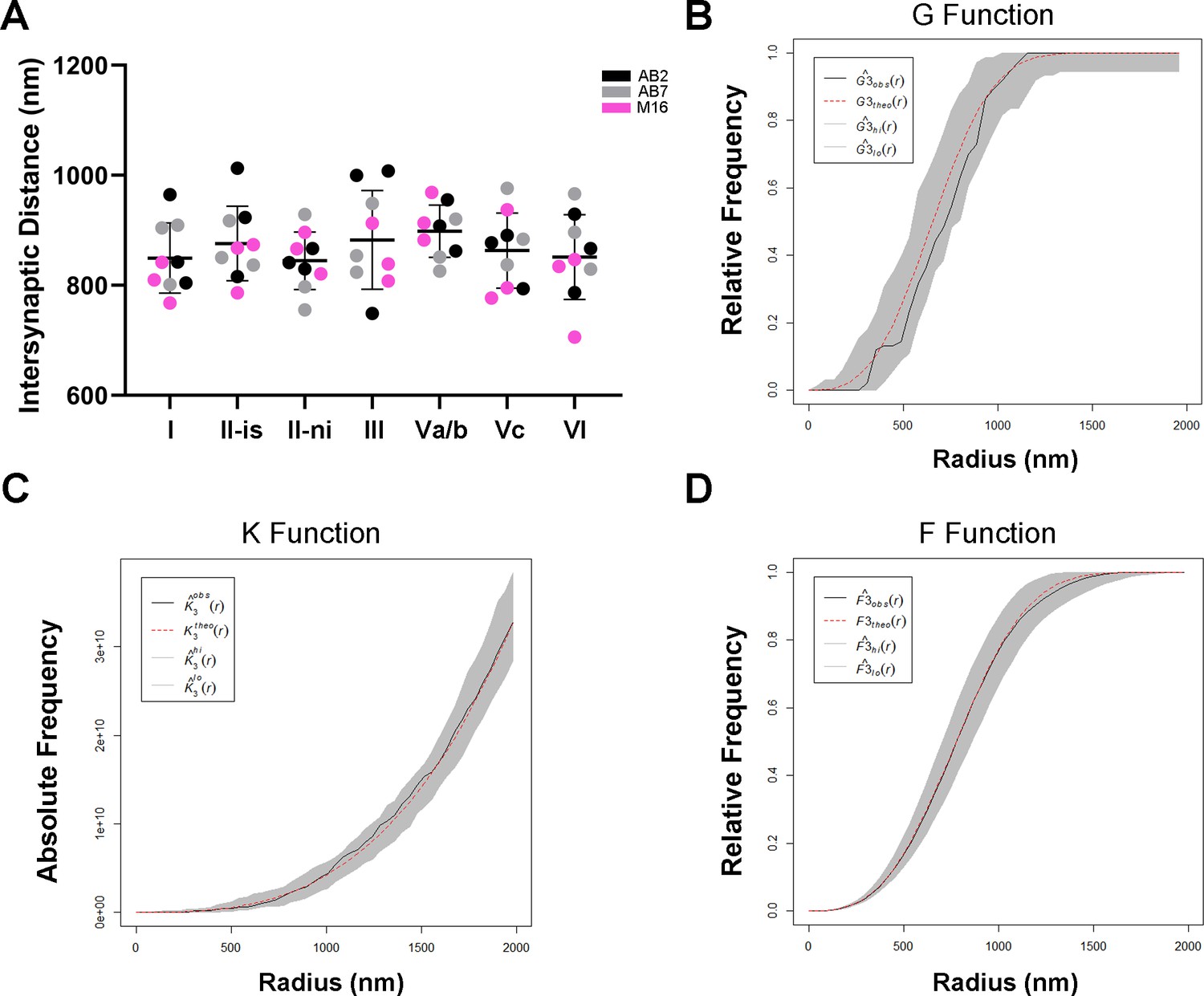
Spatial distribution analysis of synapses in the MEC.
(A) Mean intersynaptic distances (± SD) for each MEC layer. Each colored dot represents a stack of images from the analyzed cases AB2, AB7, and M16 (see Supplementary file 1p for details). No differences in the mean intersynaptic distances were found between layers (Kruskal–Wallis [KW]; p>0.05). (B–D) Representative plots for G (B), K (C), and F (D) functions. Red dashed traces correspond to a theoretical homogeneous Poisson process for each function. The black continuous traces correspond to the experimentally observed function in the sample. The shaded areas represent the envelopes of values calculated from a set of 99 simulations.
Figure 1—figure supplement 2
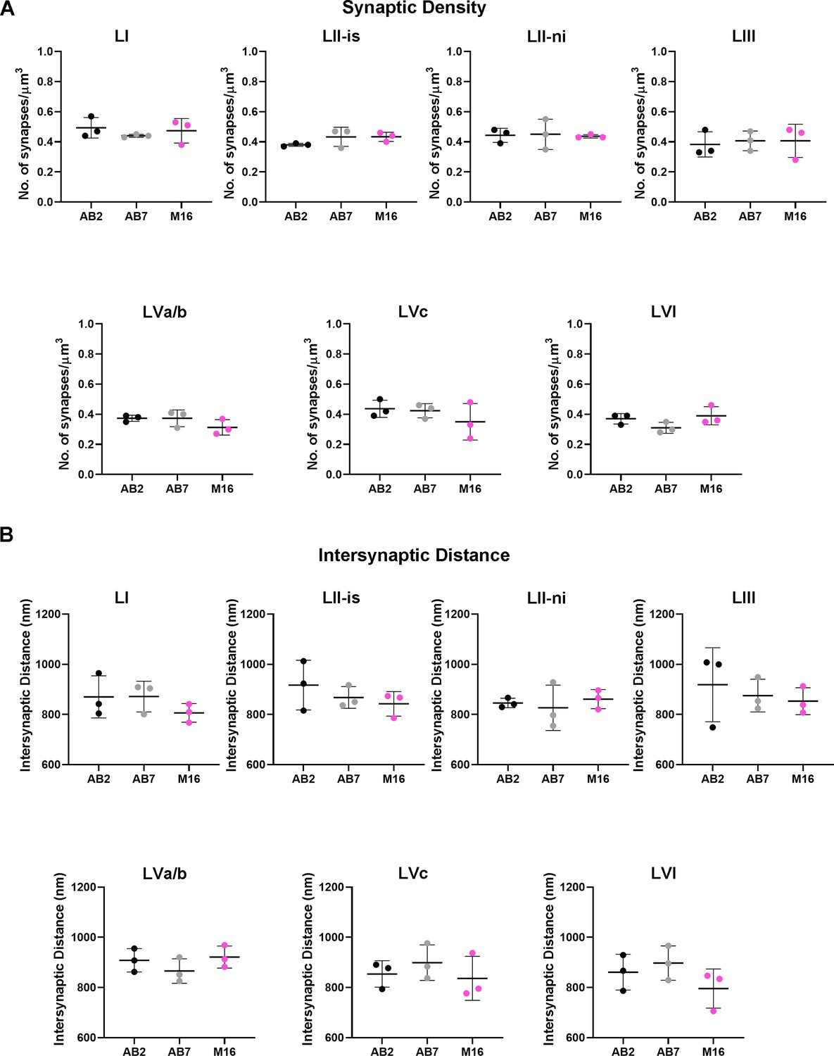
Interindividual variability of synaptic density and intersynaptic distance in the MEC.
Separated plots per layer show the synaptic density (A) and intersynaptic distance (B) per case (mean ± SD). No significant differences were found in any layer (Kruskal–Wallis [KW], p>0.05). Each colored dot represents a stack of images from the analyzed cases AB2, AB7, and M16 (see Supplementary file 1p for details). p-Values of comparisons are shown in Supplementary file 3.
Figure 2
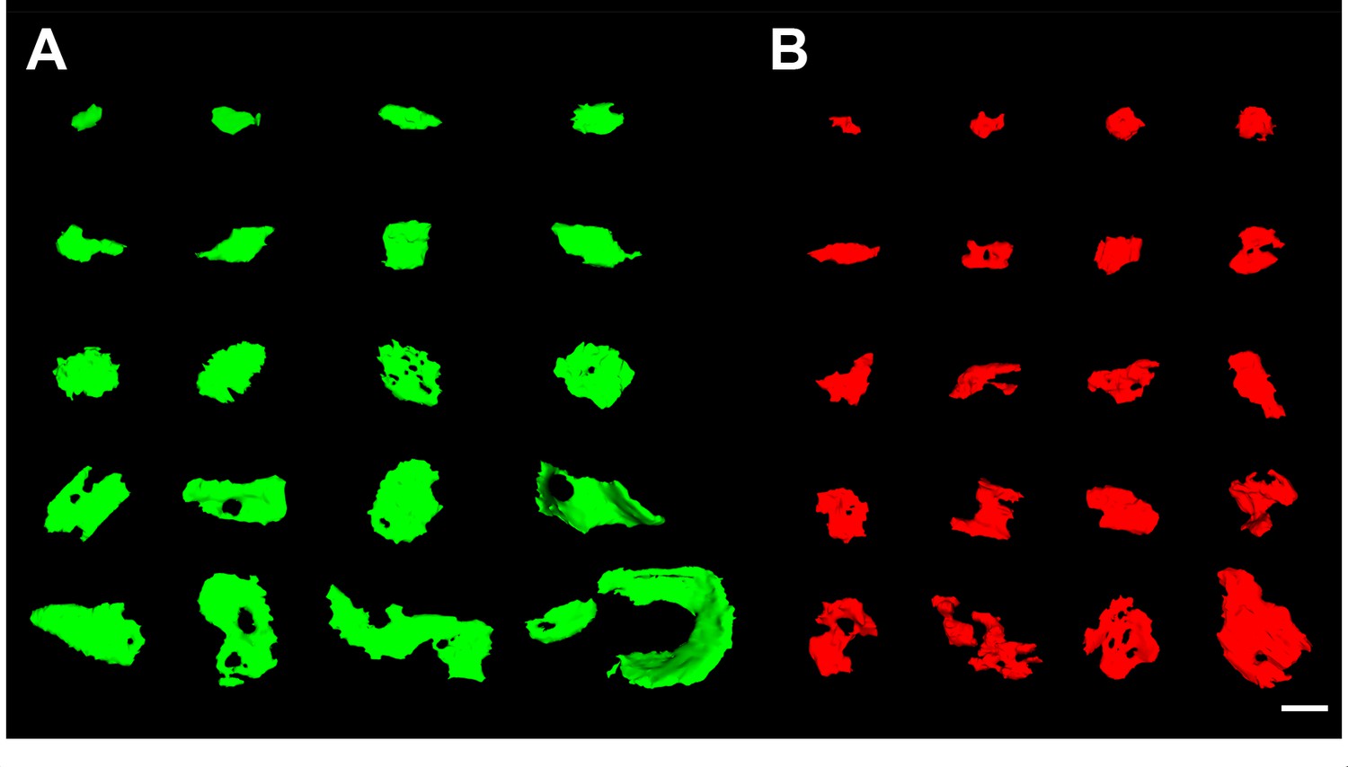
3D representative sample of synaptic apposition surfaces of asymmetric synapses and symmetric synapses in the MEC.
(A) SAS of asymmetric (green) synapses was distributed into 20 bins of equal size. An example synapse of each bin is illustrated here. (B) SAS of symmetric (red) synapses, distributed and represented as in (A). Scale bar (in B): 240 nm in (A, B).
Figure 3 with 1 supplement
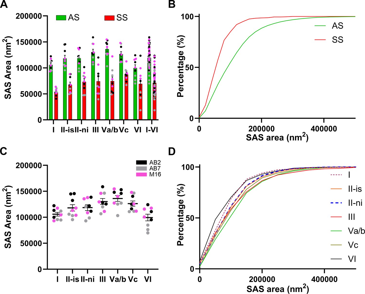
Analysis of the synaptic apposition surface (SAS) area of asymmetric synapses (AS) and symmetric synapses (SS) in the MEC.
(A) Plots of the mean SAS area (± SE) per synaptic type show larger synaptic sizes of AS (green) compared to SS (red) in all EC layers studied (Mann–Whitney [MW], p<0.0001 in layers I, II-is, II-ni, III; p<0.01 in layer Va/b and Vc; p<0.05 in layer VI; p<0.0001 considering all layers). (B) Frequency distribution graph of the SAS area illustrating that small SS (red) were more frequent than small AS (green) in all layers (Kruskal–Wallis [KW], p<0.0001). (C) Plot of the mean SAS area of AS (± SE) in all layers, with the smallest values in layer VI (Dunn’s test, p<0.05). Each colored dot represents a stack of images from the analyzed cases AB2, AB7, and M16 (see Supplementary file 1p for details). (D) Frequency distribution plot of SAS area per layer, showing that smaller sizes were more frequent in layer VI (Kolmogorov–Smirnov [KS], p<0.0001). Layer II-is had the highest interindividual variability for SAS area of AS, and statistical differences between cases were found (see detailed analysis of the variability in Figure 3—figure supplement 1 and Supplementary file 3).
Figure 3—figure supplement 1
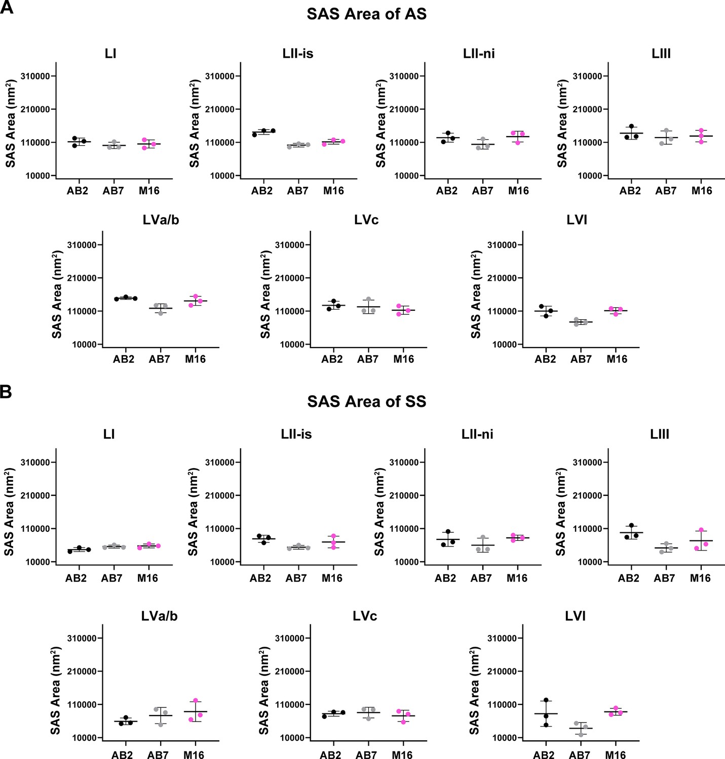
Interindividual variability of synaptic apposition surface (SAS) area of asymmetric synapses (AS) and symmetric synapses (SS) in the MEC.
Separated plots per layer show the SAS area of AS (A) and SS (B) per case (mean ± SD). In layer II-is, AB2 shows a larger SAS area of AS than AB7 (Dunn’s test, p<0.05). No significant differences were found in the remaining comparisons (Dunn’s test, p>0.05). Each colored dot represents a stack of images from the analyzed cases AB2, AB7, and M16 (see Supplementary file 1p for details). p-Values of comparisons are shown in Supplementary file 3.
Figure 4 with 5 supplements
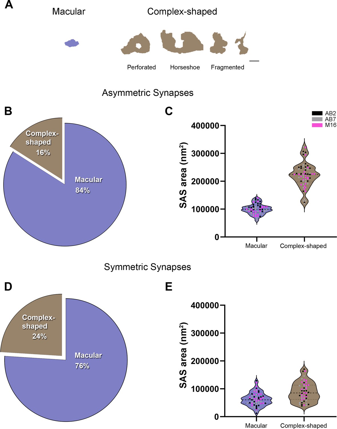
Analysis of the synaptic shape of asymmetric synapses (AS) and symmetric synapses (SS) in the MEC.
(A) Schematic representations of the different types of synapses based on the shape of their synaptic junction: macular, perforated, horseshoe, and fragmented. Perforated, horseshoe, and fragmented were grouped into complex-shaped synapses. Scale bar: 250 nm. (B) Pie chart showing the proportion of AS presenting macular and complex-shaped synapses in all layers. Macular synapses represented the most common shape (84%). (C) Mean plot of the synaptic apposition surface (SAS) area (± SE) of macular and complex-shaped AS considering all layers. Complex-shaped AS were larger than macular synapses (Mann-Whitney [MW], p<0.0001). Each dot represents a stack of images from the analyzed cases AB2, AB7, and M16 (see Supplementary file 1p for details). (D) Pie chart showing the proportion of SS presenting macular and complex-shaped synapses in all layers. Once again, macular synapses represented the most common shape (76%). (E) Mean plot of the SAS area (± SE) of macular and complex-shaped SS considering all layers. Complex-shaped SS were larger than macular synapses (MW, p<0.0001). See Figure 4—figure supplement 1 for a detailed description of each layer. The statistical interindividual variability test for SAS area of complex AS showed differences between cases in layer VI (see detailed analysis of the variability in Figure 4—figure supplement 5 and Supplementary file 3).
Figure 4—figure supplement 1
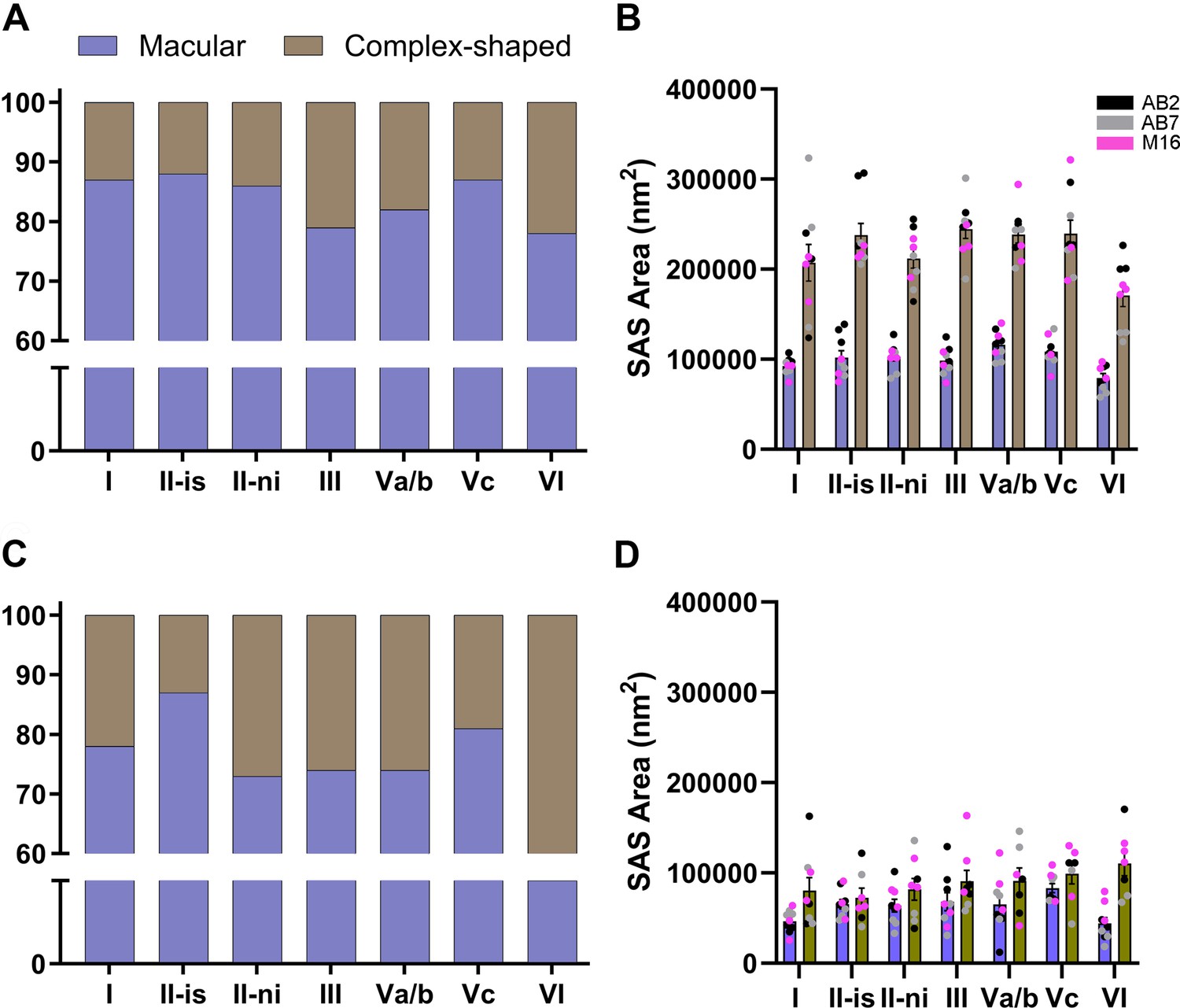
Analysis of asymmetric (AS; A, B) and symmetric (SS; C, D) synapse shape in the MEC, per layer.
(A) Proportion of macular and complex-shaped AS (i.e., perforated, horseshoe, and fragmented). Layer VI presented the lowest percentage of macular synapses (78%; χ2, p<0.0001). (B) Plot of the mean synaptic apposition surface (SAS) area (± SE) of macular and complex-shaped AS. Complex-shaped AS were significantly larger than macular synapses (Mann–Whitney [MW], p<0.05 in all layer comparisons). Each dot represents a stack of images from the analyzed cases AB2, AB7, and M16 (see Supplementary file 1p for details). (C) Proportion of macular and complex-shaped SS. Again, layer VI presented the lowest percentage of macular synapses (59%). (D) Plot of the mean SAS area (± SE) of macular and complex-shaped SS. Complex-shaped SS were larger than macular synapses in all layers; however, only layer I and layer VI presented significant differences (MW, p<0.05).
Figure 4—figure supplement 2
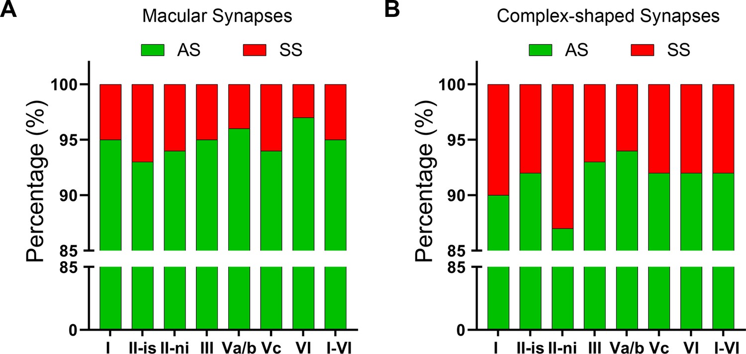
Proportion of asymmetric synapses (AS) and symmetric synapses (SS) in macular and complex-shaped synapses.
(A) Proportion of AS and SS macular synapses. The overall AS:SS ratio of macular synapses was 95:5. No significant differences were found between layers (χ2, p>0.0001). (B) Proportion of AS and SS complex-shaped synapses. The overall ratio on complex-shaped synapses was 92:8. No significant differences were found between the layers (χ2, p>0.0001).
Figure 4—figure supplement 3

Comparison of the synaptic apposition surface (SAS) of macular (A, B) and complex-shaped (C, D) asymmetric synapses (AS) between MEC layers.
(A) Plots of the mean SAS area (± SE) of macular AS per layer. Layer VI had the smallest macular synapses of all layers (Dunn’s test, p<0.05). Each dot represents a stack of images from the analyzed cases AB2, AB7, and M16 (see Supplementary file 1p for details). (B) Frequency distribution plot of SAS area per layer, for macular synapses, showing that smaller sizes were more frequent in layer VI (Kolmogorov–Smirnov [KS], p<0.0001). (C) Plots of the mean SAS area (± SE) of complex-shaped AS per layer. Again, layer VI had the smallest complex-shaped synapses of all layers (Dunn’s test, p<0.05). (D) Frequency distribution plot of SAS area per layer, for complex synapses, showing that smaller sizes were more frequent in layer VI (KS, p<0.0001).
Figure 4—figure supplement 4
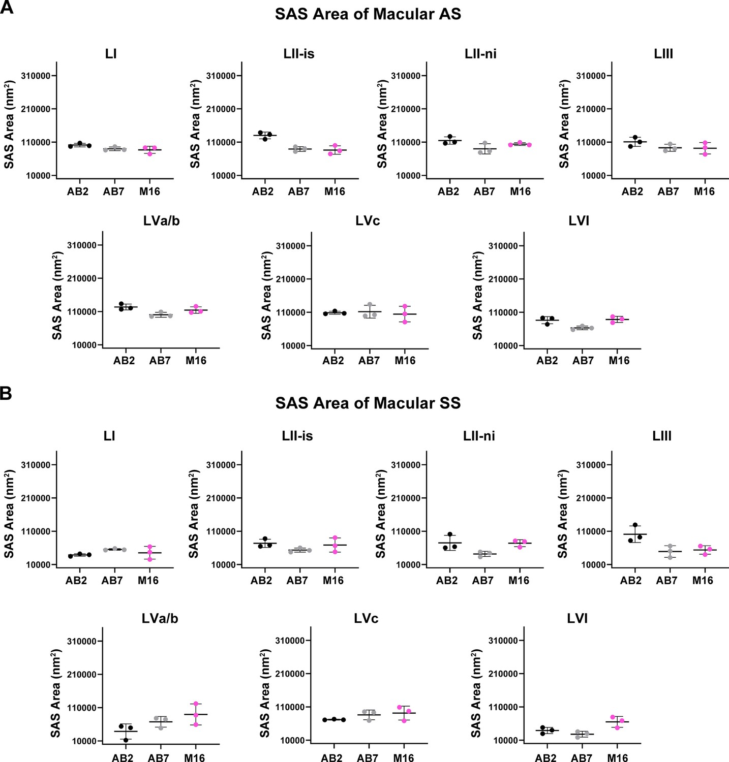
Interindividual variability of synaptic apposition surface (SAS) area of macular asymmetric synapses (AS) and symmetric synapses (SS) in the MEC.
Separated plots per layer show the SAS area of macular AS (A) and SS (B) per case (mean ± SD). No significant differences were found in any layer (Kruskal–Wallis [KW], p>0.05). Each colored dot represents a stack of images from the analyzed cases AB2, AB7, and M16 (see Supplementary file 1p for details). p-Values of comparisons are shown in Supplementary file 3.
Figure 4—figure supplement 5
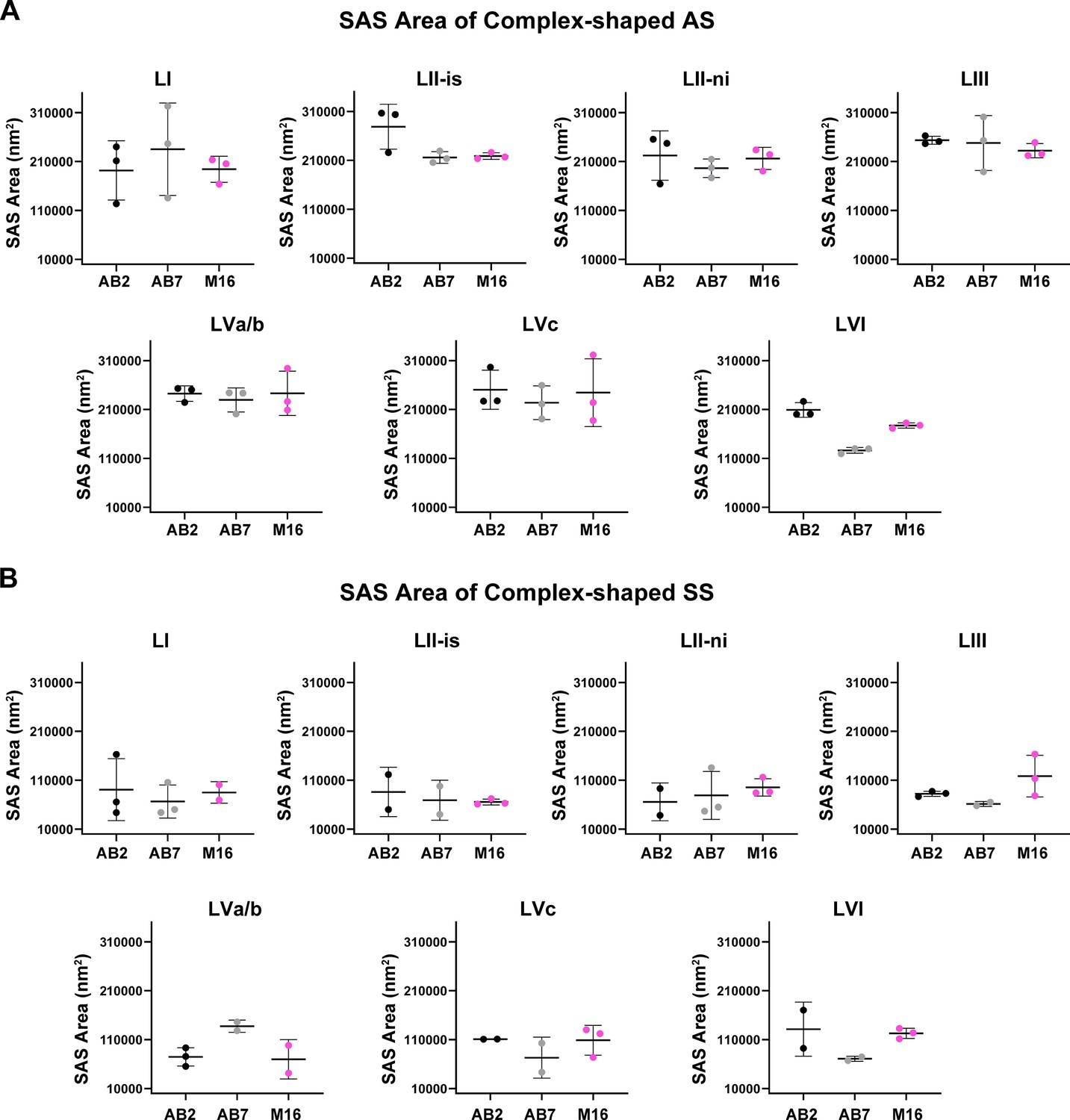
Interindividual variability of synaptic apposition surface (SAS) area of complex-shaped asymmetric synapses (AS) and symmetric synapses (SS) in the MEC.
Separated plots per layer show the SAS area of complex-shaped AS (A) and SS (B) per case (mean ± SD). In LVI, AB2 have larger SAS area of complex-shaped AS than AB7 (Dunn’s test, p<0.05). No significant differences were found in the rest of the layers (Dunn’s test, p>0.05). Each colored dot represents a stack of images from the analyzed cases AB2, AB7, and M16 (see Supplementary file 1p for details). p-Values of comparisons are shown in Supplementary file 3.
Figure 5
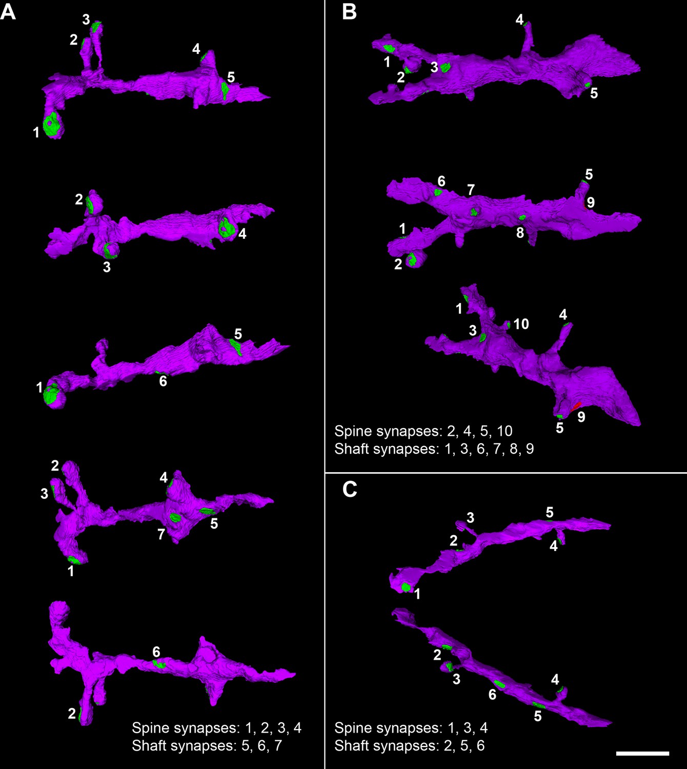
Examples of 3D reconstructed dendritic segments (purple) establishing asymmetric (green) and symmetric (red) synapses.
Three different dendritic segments (A–C) illustrating synaptic junctions at different view angles. Numbers correspond to the same synapse in each dendritic segment. Note the different sizes and shapes of the synaptic junctions on each dendritic segment. The dendritic surface of the shaft presents relatively few synaptic contacts. Scale bar (in C): 3.6 µm in (A–C). See also Figure 13.
Figure 6 with 3 supplements
Distribution of synapses according to their postsynaptic target in each MEC layer.
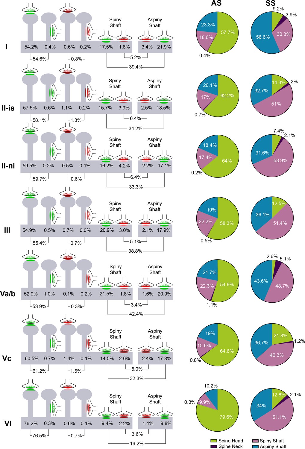
(Left) Schematic representation of the distribution of synapses according to their postsynaptic element: data refer to the percentages of axospinous (i.e., head and neck of dendritic spines) and axodendritic (spiny and aspiny shafts) asymmetric (green) and symmetric (red) synapses (see Supplementary file 1j for detailed information regarding the absolute number of each synaptic type). (Right) Pie charts to illustrate the proportion of asymmetric synapses (AS) (green) and symmetric synapses (SS) (red) according to their location as axospinous synapses (i.e., on the head or neck of the spine) or axodendritic synapses (i.e., spiny or aspiny shafts) in each MEC layer (see legend). AS were preferentially formed on dendritic spine heads (63%), although differences were observed between layers (χ2, p<0.0001). Supplementary file 1k shows the percentage and absolute number of each synaptic type.
Figure 6—figure supplement 1
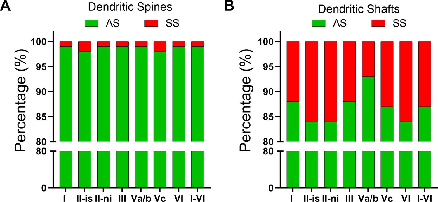
Proportion of asymmetric synapses (AS) and symmetric synapses (SS) in dendritic spines and shafts.
(A) Proportion of AS and SS synapses on dendritic spines. The overall AS:SS ratio was 99:1. No significant differences were found between the layers (χ2, p>0.0001). (B) Proportion of AS and SS on dendritic shafts. The overall ratio was 87:13. No significant differences were found between the layers (χ2, p>0.0001).
Figure 6—figure supplement 2
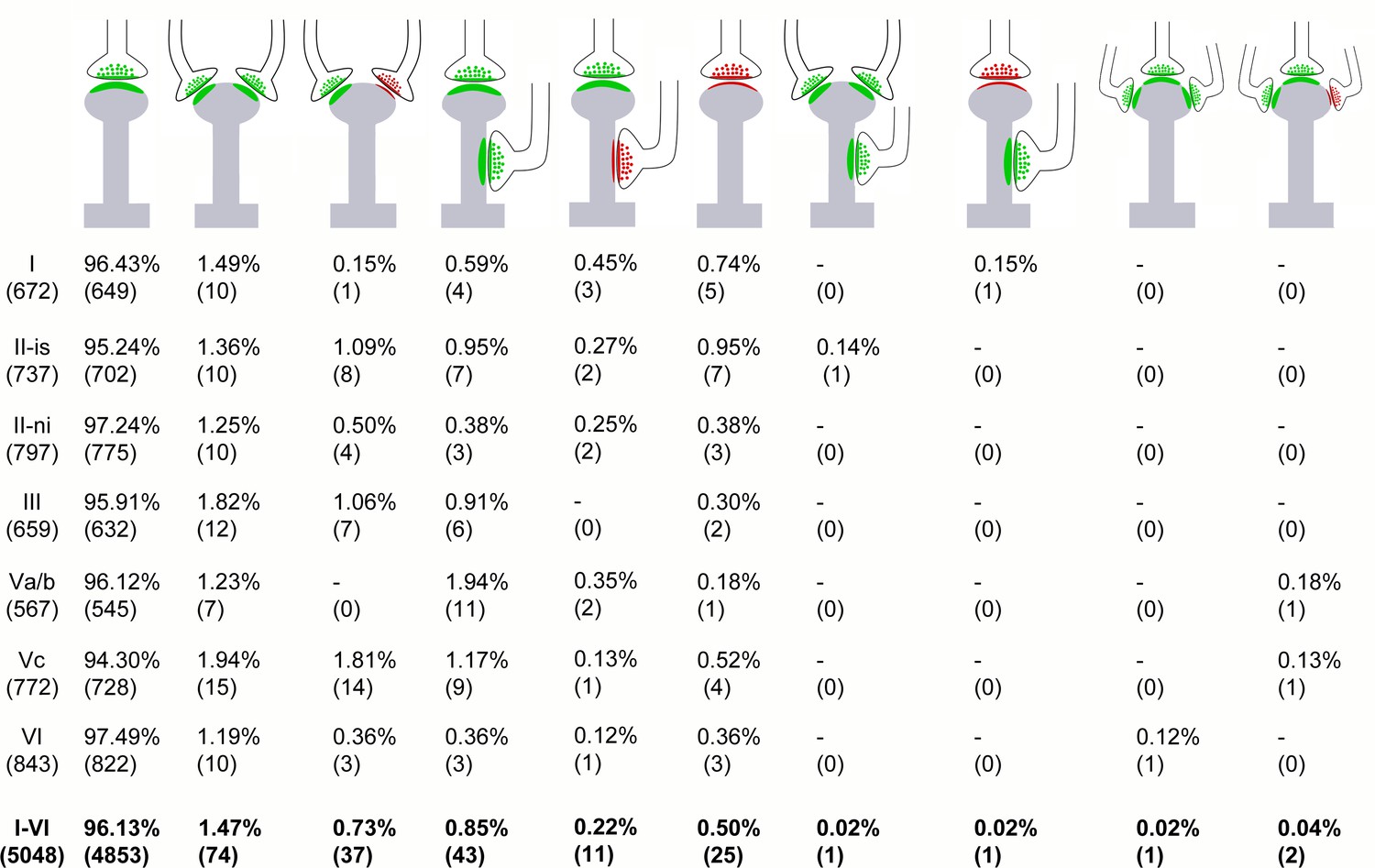
Schematic representation of the proportion of single and multisynaptic spines in all MEC layers.
Data in parentheses refer to the absolute number of spines.
Figure 6—figure supplement 3
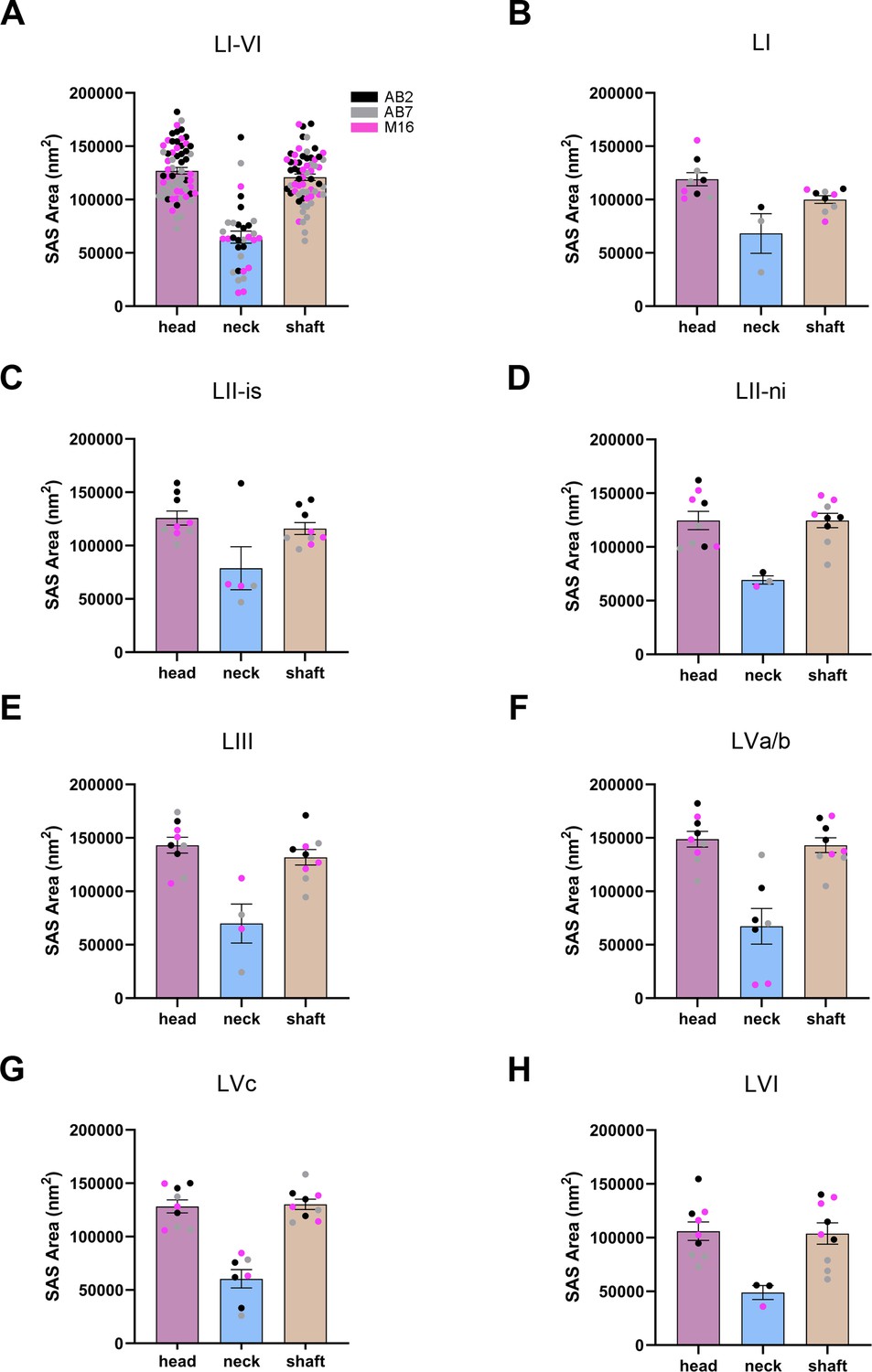
Analysis of synaptic apposition surface (SAS) of asymmetric synapses (AS) for each of the postsynaptic targets in the MEC.
(A) Plots of the mean SAS area (± SE) for AS established on spine heads, necks, and dendritic shafts, considering all layers. Each dot represents a stack of images from the analyzed cases AB2, AB7, and M16 (see Supplementary file 1p for details). Synapses established on the spine neck were significantly smaller (Dunn’s test, p<0.001). (B–H) Plots of the mean SAS area (± SE) for AS established on spine heads, necks, and dendritic shafts of each MEC layer.
Figure 7 with 2 supplements
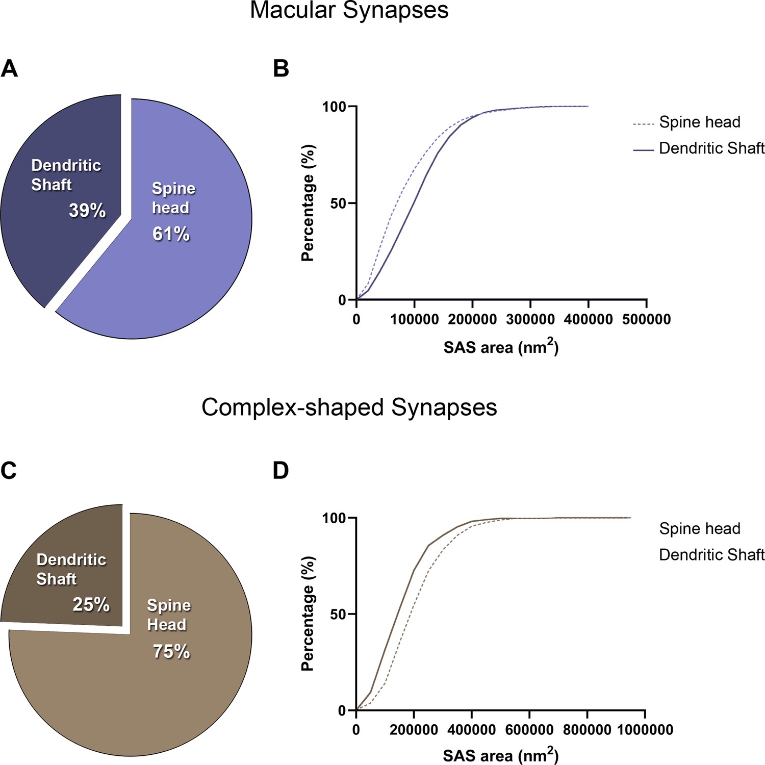
Analysis of the distribution of macular and complex-shaped asymmetric synapses (AS) on postsynaptic targets.
(A) Pie chart illustrating the proportion of macular AS on spine heads and dendritic shafts, considering all layers. This distribution is similar to the general proportion of AS on spine heads and shafts, regardless of the synaptic shape (63:37). (B) Frequency distribution plot of the synaptic apposition surface (SAS) of macular AS on spine heads and dendritic shafts, showing that smaller macular AS were more frequent on spine heads (Kolmogorov–Smirnov [KS], p<0.0001). (C) Pie chart illustrating the proportion of complex-shaped AS on spine heads and dendritic shafts, considering all layers. In this case, the proportion of complex synapses on spine heads is higher than what would be expected from the general distribution (χ2, p<0.0001). (D) Frequency distribution plot of the SAS of complex-shaped AS on spine heads and dendritic shafts, showing that smaller complex-shaped AS were more frequent on dendritic shafts (KS, p<0.0001). See Figure 7—figure supplements 1 and 2 for a detailed description of each layer.
Figure 7—figure supplement 1
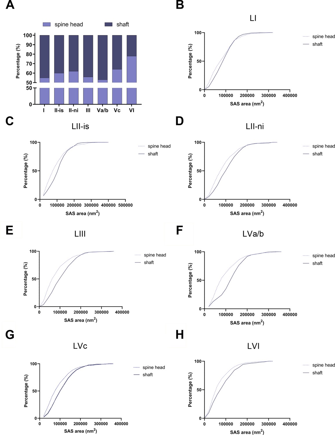
Analysis of the distribution of macular asymmetric synapses (AS) on postsynaptic targets, per MEC layer.
(A) Distribution of macular AS on spine heads and dendritic shafts in each layer. Layer VI exhibited the highest proportion of macular AS established on spine heads (78%; χ2, p<0.0001). (B–H) Frequency distribution plots of the synaptic apposition surface (SAS) of macular AS established on spine heads and dendritic shafts, per cortical layer.
Figure 7—figure supplement 2
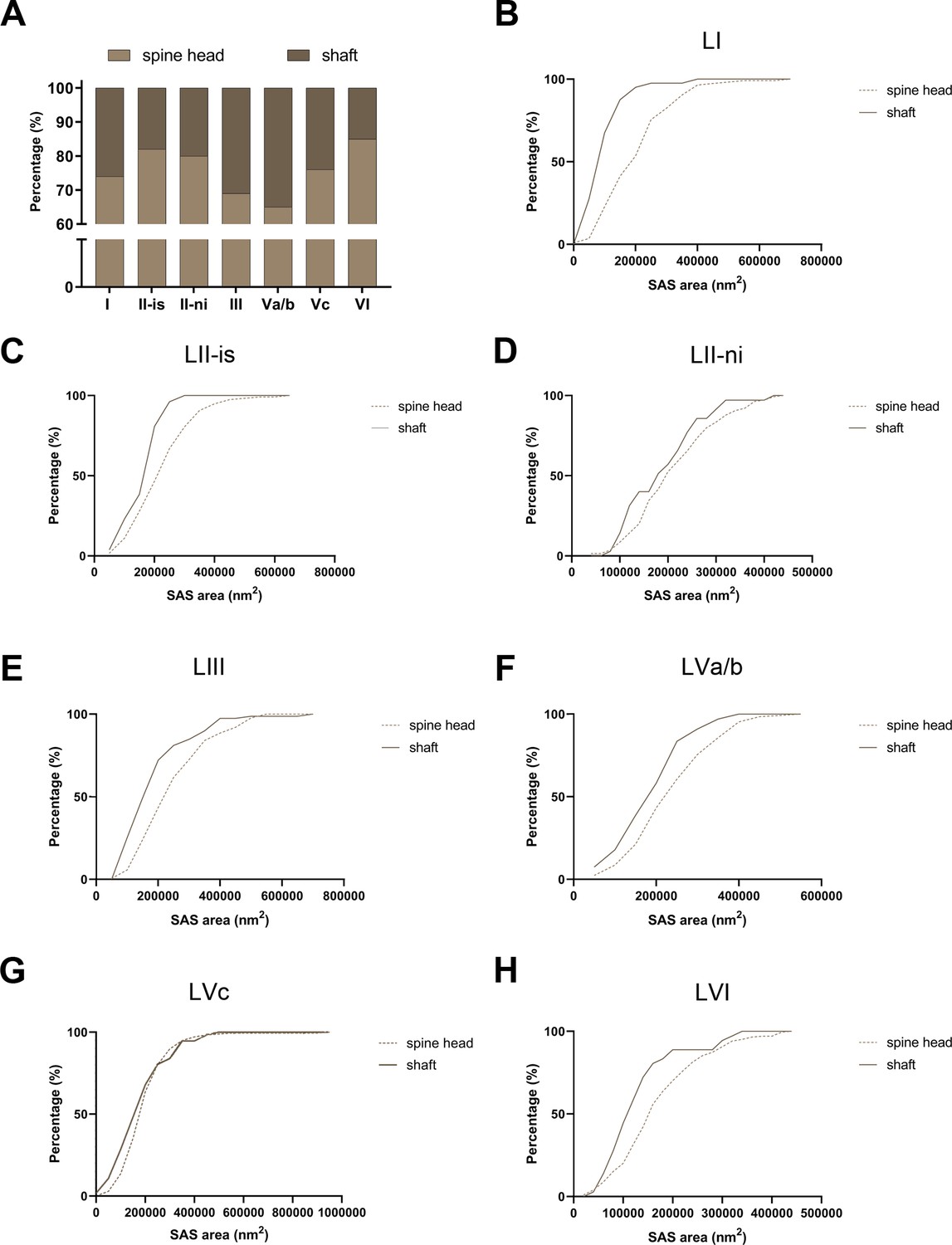
Analysis of the distribution of complex-shaped asymmetric synapses (AS) on postsynaptic targets, per MEC layer.
(A) Distribution of complex-shaped AS on spine heads and dendritic shafts in each layer. Layer VI exhibited the highest proportion of complex-shaped AS established on spine heads (85%, χ2, p<0.0001). (B–H) Frequency distribution plots of the synaptic apposition surface (SAS) of complex-shaped AS established on spine heads and dendritic shafts, per cortical layer.
Figure 8
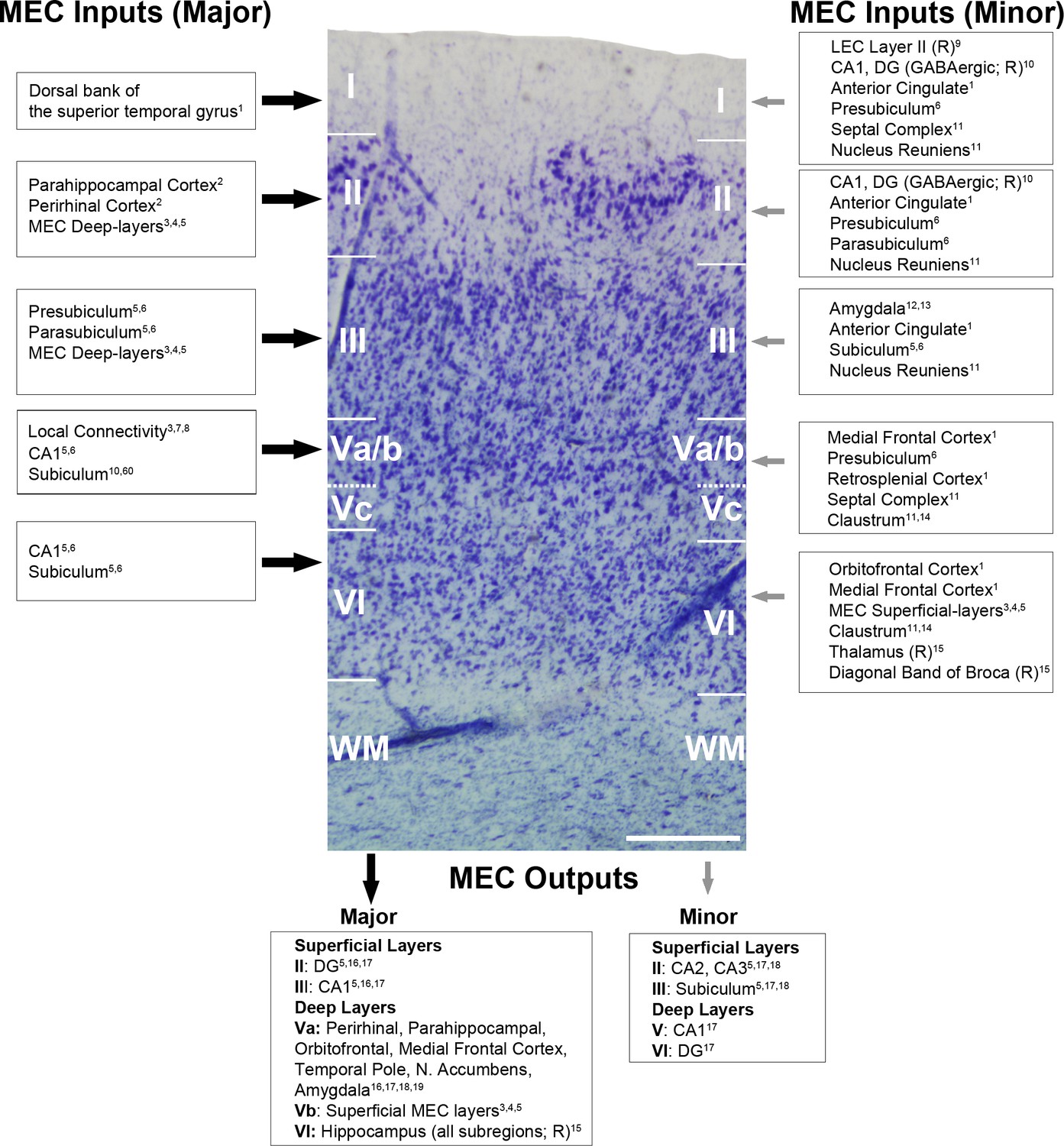
Main extrinsic and intrinsic connections of the MEC.
Major and minor MEC inputs and outputs have been represented with large (black) and small (gray) arrows, respectively. Connections have been illustrated on a photograph of a Nissl-stained coronal section from the human MEC, where all layers can be individually identified. The data mainly come from primates and rodents (marked as ‘R’ in the figure, for those connections only described in rodents). Scale bar indicates 415 µm. References: 1Insausti and Amaral, 2008; 2Maass et al., 2015; 3Chrobak and Amaral, 2007; 4Sürmeli et al., 2016; 5Nilssen et al., 2019; 6Witter and Amaral, 2021; 7Gerlei et al., 2021; 8Rozov et al., 2020; 9Vandrey et al., 2022; 10Melzer et al., 2012; 11Insausti et al., 1987; 12Pitkänen et al., 2002; 13Roesler and McGaugh, 2022; 14Kitanishi and Matsuo, 2017; 15Ben-Simon et al., 2022; 16Insausti and Amaral, 2012; 17Witter and Amaral, 1991; 18Muñoz and Insausti, 2005; 19Ohara et al., 2021.
Figure 9
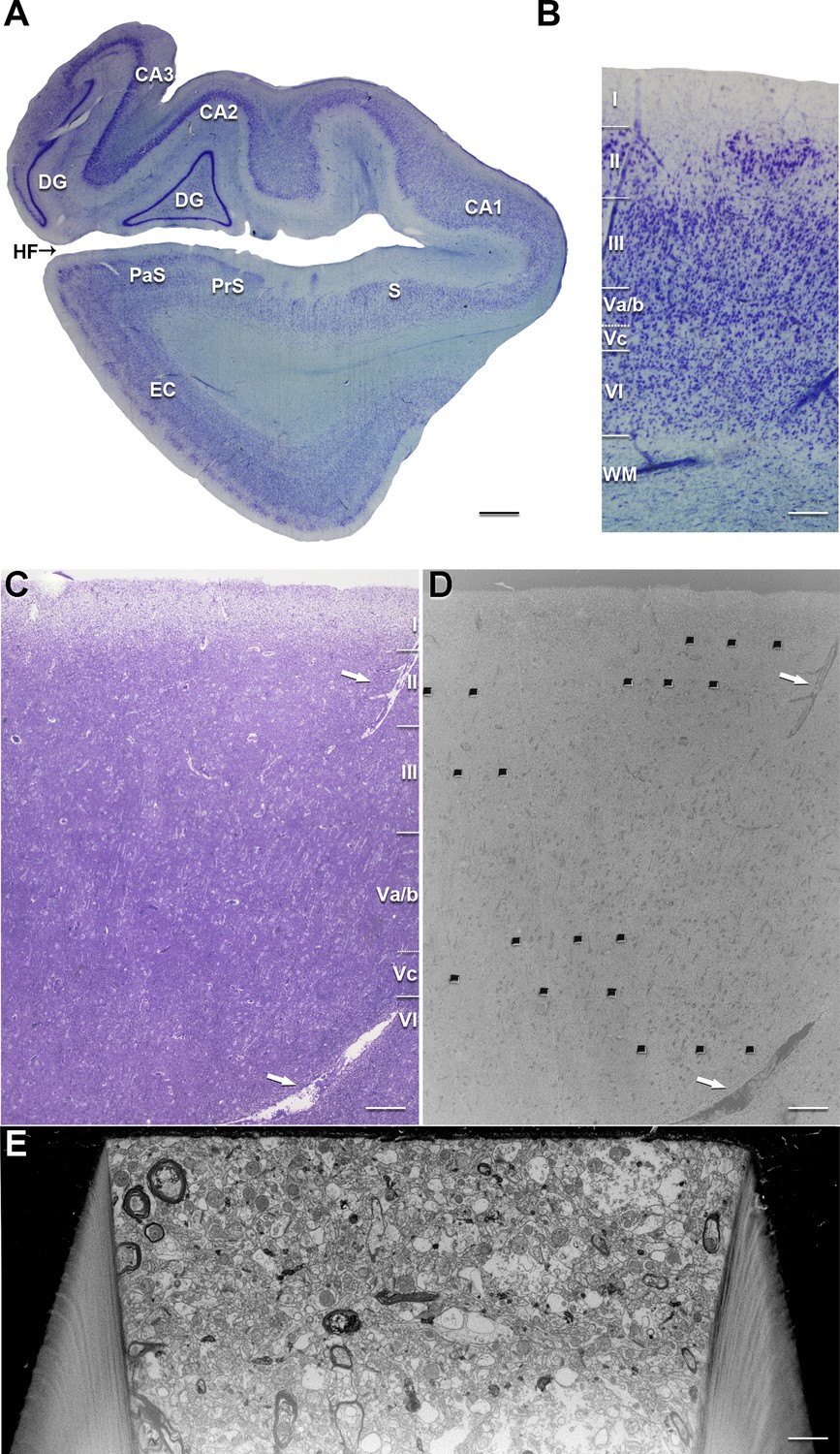
Correlative light/electron microscopy of the MEC layers.
(A) Low-power photograph of a coronal section from the human hippocampal formation and entorhinal cortex. (B) Higher magnification of the MEC shown in (A), to illustrate the laminar pattern (layers I to VI are indicated). This image was reused from Figure 8. The delimitation of layers is based on the toluidine blue-stained semithin section (C), adjacent to the block for focused ion beam FIB/SEM imaging (D). (D) SEM image illustrating the block surface with trenches made in the neuropil of MEC layers. Arrows in (A) and (B) mark the same blood vessel, allowing the regions of interest to be accurately located. (E) SEM image showing the front of a trench made to acquire the FIB/SEM stack of images. CA1: cornu ammonis 1; CA2: cornu ammonis 2; CA3: cornu ammonis 3; DG: dentate gyrus; EC: entorhinal cortex; HF: hippocampal fissure; PaS: parasubiculum; PrS: presubiculum; S: subiculum. Scale bar: 1.4 mm in (A), 260 µm in (B), 175 µm in (C), 165 µm in (D) and 2 µm in (E).
Figure 10 with 6 supplements
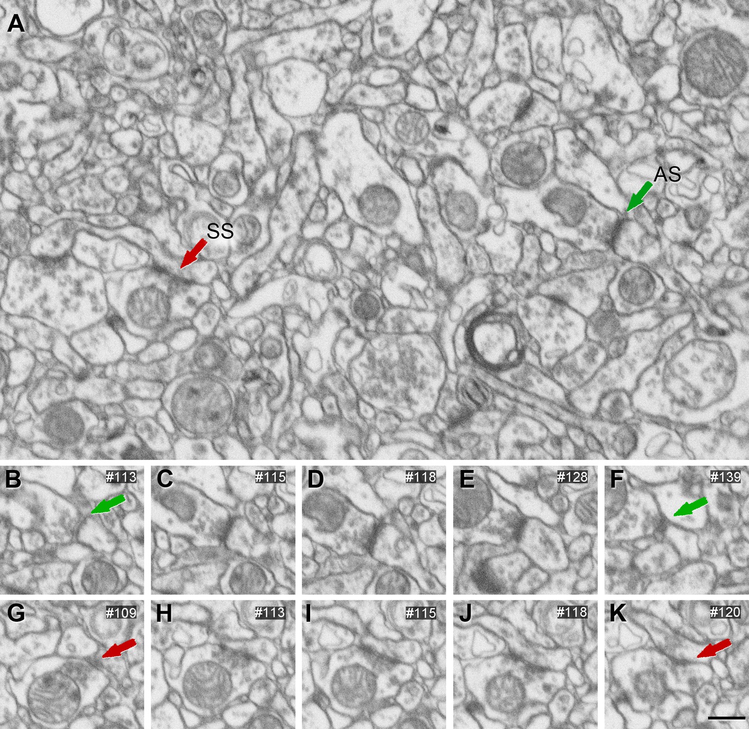
Focused ion beam FIB/SEM images from layer Va/b.
(A) Two synapses are indicated as examples of asymmetric (AS, green arrow) and symmetric (SS, red arrow) synapses. Figure 10—figure supplements 1–6 show FIB/SEM images from the neuropil of the rest of the layers. (B–F) FIB/SEM serial images of the AS indicated in (A). (G–K) FIB/SEM serial images of the SS indicated in (A). Synapse classification was based on the examination of full sequences of serial images. Scale bar (in K): 500 nm for (A–K).
Figure 10—figure supplement 1
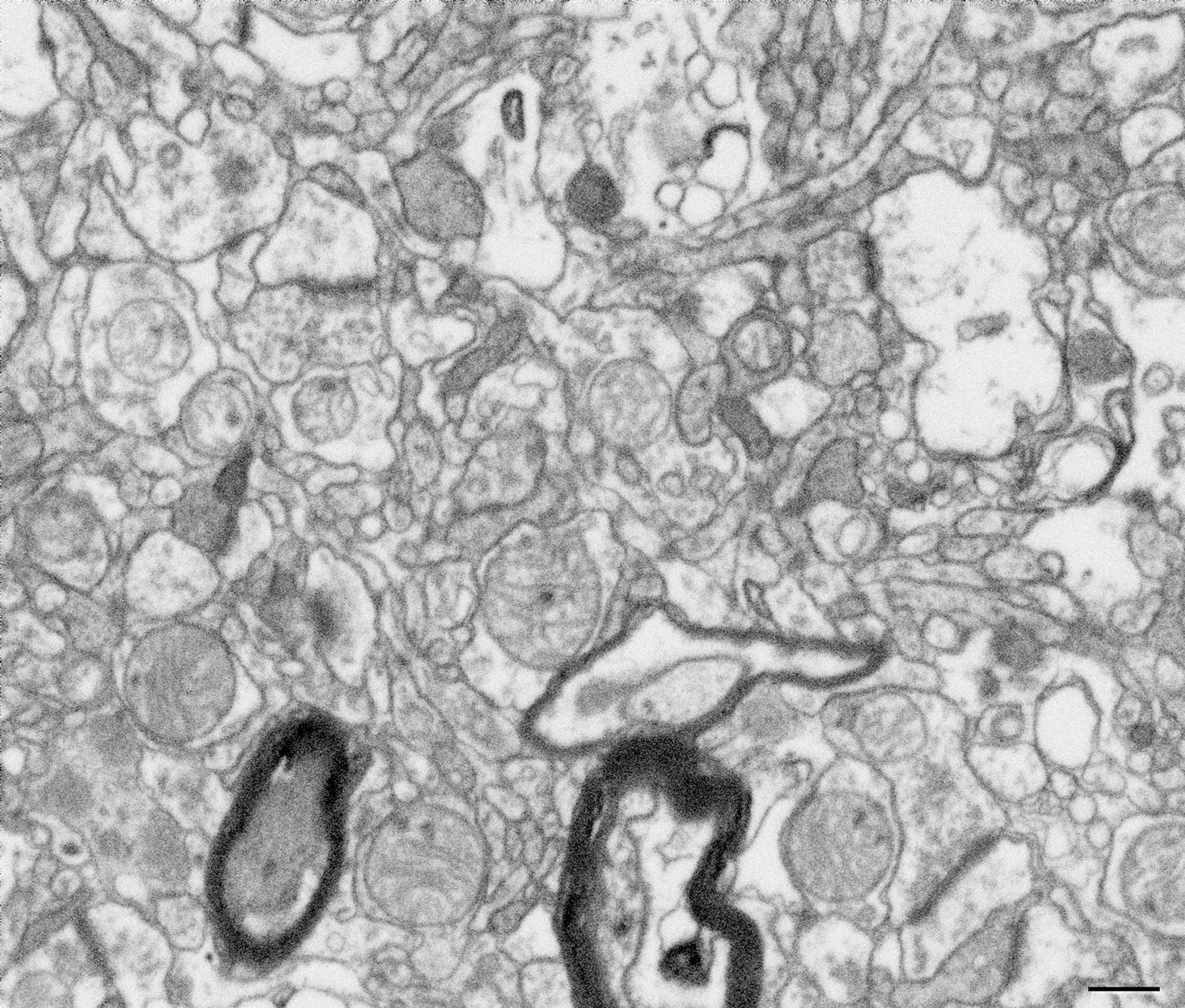
Ultrastructure of the neuropil in layer I.
Focused ion beam FIB/SEM image resolution in the xy plane was 5 nm/pixel. Resolution in the z-axis (section thickness) was 20 nm. Scale bar indicates 575 nm.
Figure 10—figure supplement 2
Ultrastructure of the neuropil in layer II-is.
Focused ion beam FIB/SEM image resolution in the xy plane was 5 nm/pixel. Resolution in the z-axis (section thickness) was 20 nm. Scale bar indicates 575 nm.
Figure 10—figure supplement 3
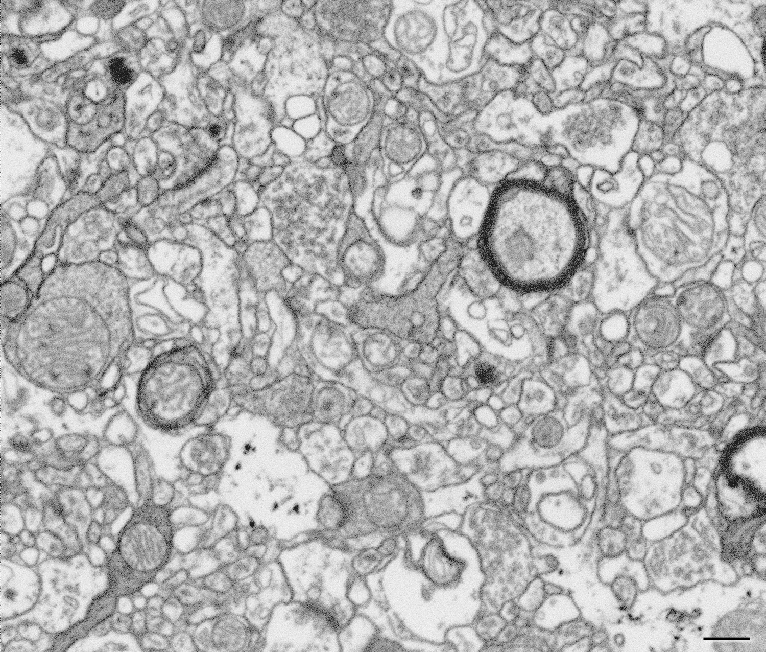
Ultrastructure of the neuropil in layer II-ni.
Focused ion beam FIB/SEM image resolution in the xy plane was 5 nm/pixel. Resolution in the z-axis (section thickness) was 20 nm. Scale bar indicates 575 nm.
Figure 10—figure supplement 4
Ultrastructure of the neuropil in layer III.
Focused ion beam FIB/SEM image resolution in the xy plane was 5 nm/pixel. Resolution in the z-axis (section thickness) was 20 nm. Scale bar indicates 575 nm.
Figure 10—figure supplement 5
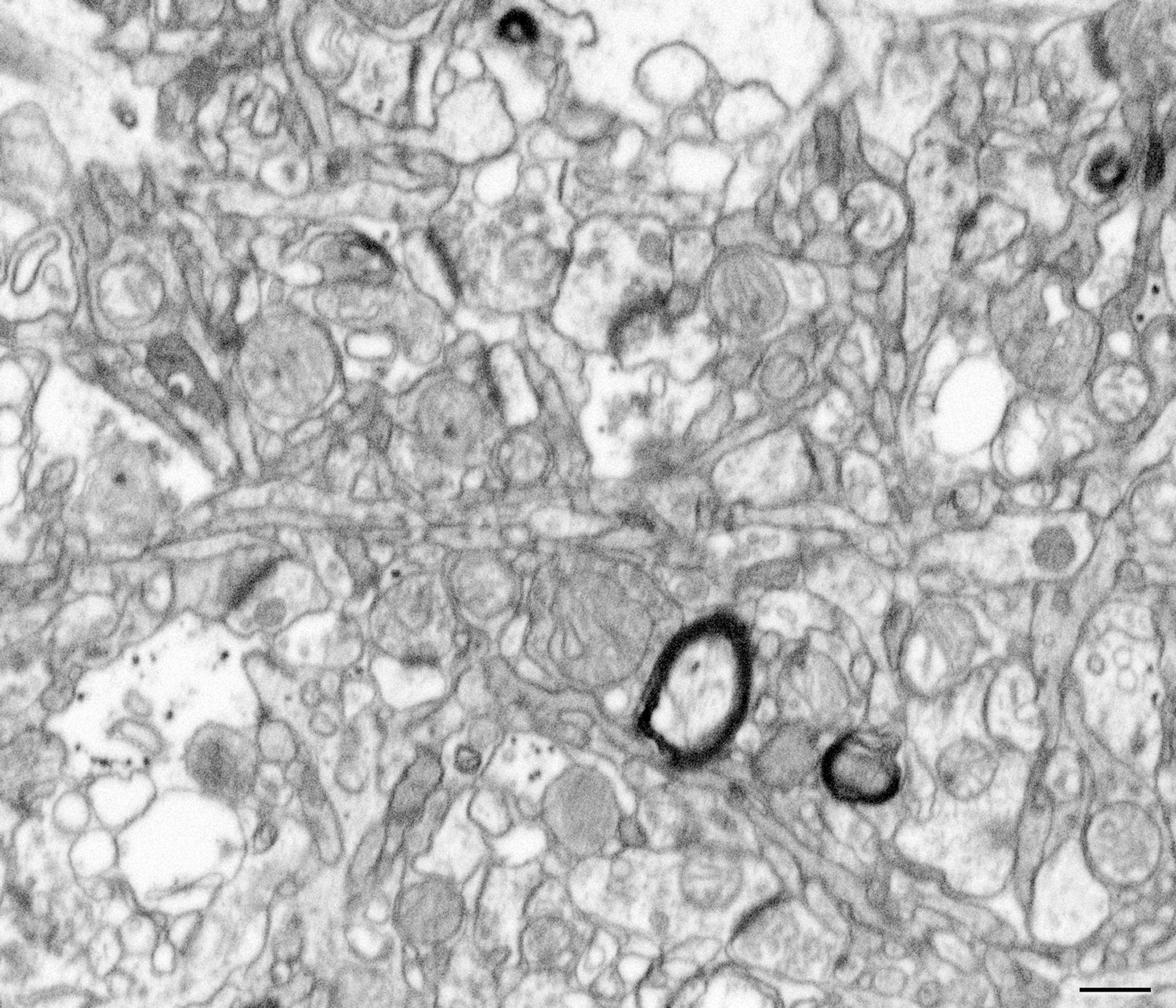
Ultrastructure of the neuropil in layer Vc.
Focused ion beam FIB/SEM image resolution in the xy plane was 5 nm/pixel. Resolution in the z-axis (section thickness) was 20 nm. Scale bar indicates 575 nm.
Figure 10—figure supplement 6

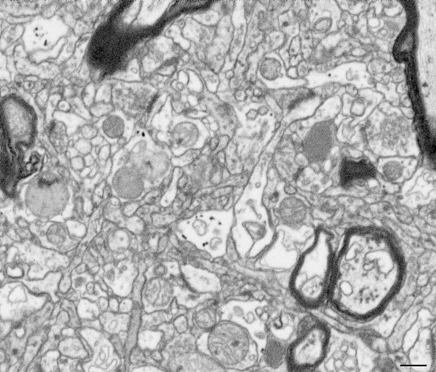
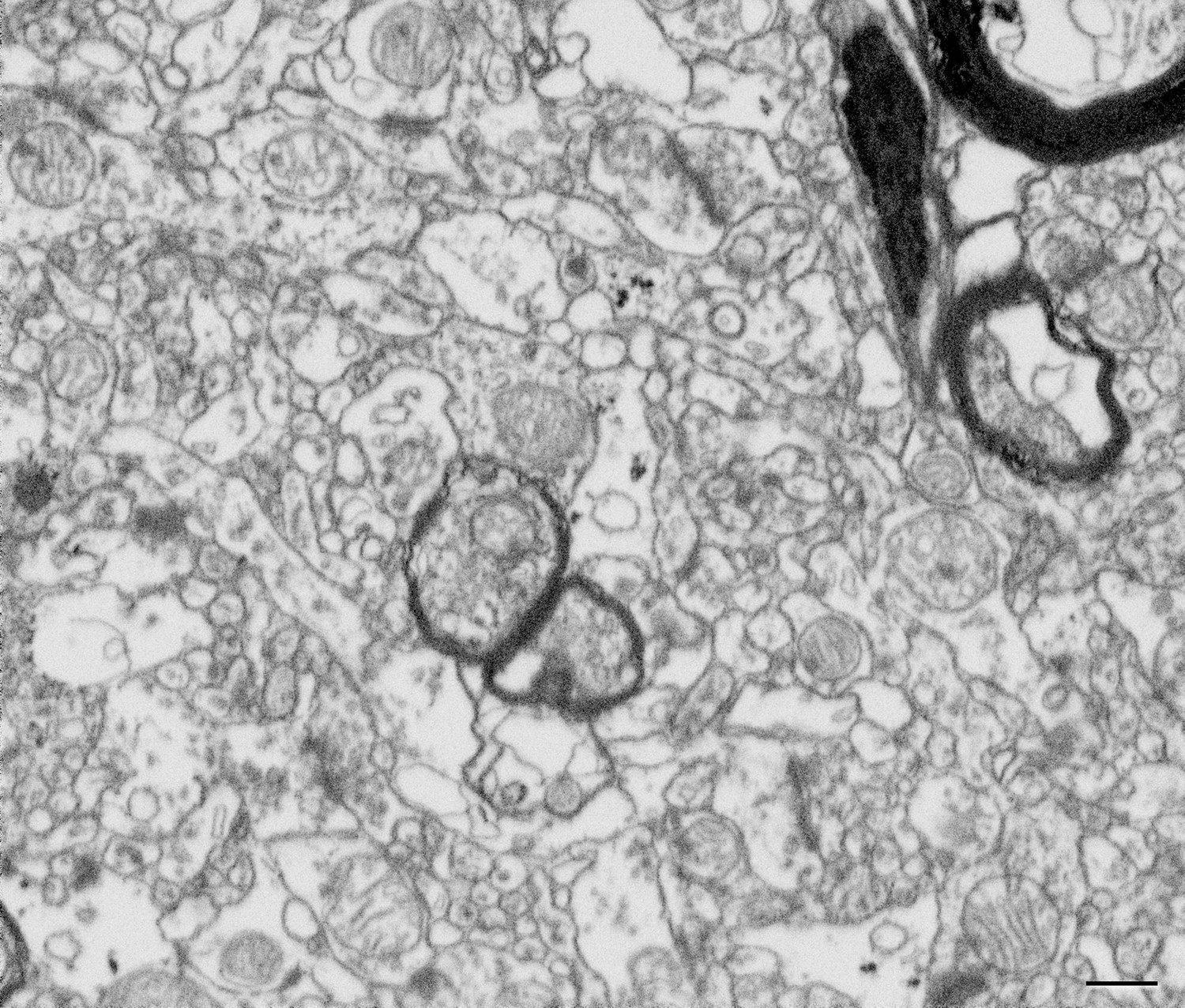
Ultrastructure of the neuropil in layer VI.
Focused ion beam FIB/SEM image resolution in the xy plane was 5 nm/pixel. Resolution in the z-axis (section thickness) was 20 nm. Scale bar indicates 575 nm.
Figure 11
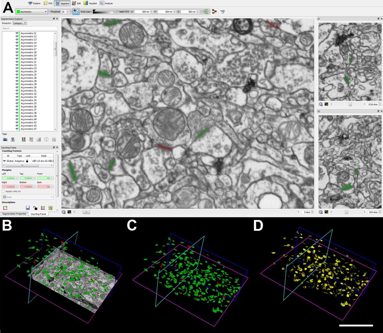
Screenshots of the EspINA software user interface.
(A) In the main window, sections are viewed through the xy plane, and the other two orthogonal planes, yz and xz, are shown in adjacent windows (right). (B–D) 3D views showing: the three orthogonal planes and the 3D reconstruction of asymmetric synapses (AS) (green) and symmetric synapses (SS) (red) segmented synapses (B); only the reconstructed synapses (C); and the synaptic apposition surface (SAS) for each reconstructed synapse (D, in yellow). Scale bar (in D): 11 µm for (B–D).
Figure 12

Extraction of the synaptic apposition surface (SAS).
(A–D) An example of focused ion beam FIB/SEM serial images showing an asymmetric synapses (AS) (in green). (E, F) 3D Reconstruction of the AS, indicated in (A–D), in different rotation planes. A central perforation can be observed. (G, H) Automatically generated SAS of the reconstructed synapse in the same rotation planes as in (E, F). The obtained SAS reproduces the profile and the irregular curvature of the 3D reconstructed synapse, in which the same central perforation can be observed. SAS includes both the active zone and the postsynaptic density (PSD) of the 3D segmented synapse. Scale bar (in H): 500 nm in (A–D); 165 nm in (E–H).
Figure 13 with 1 supplement
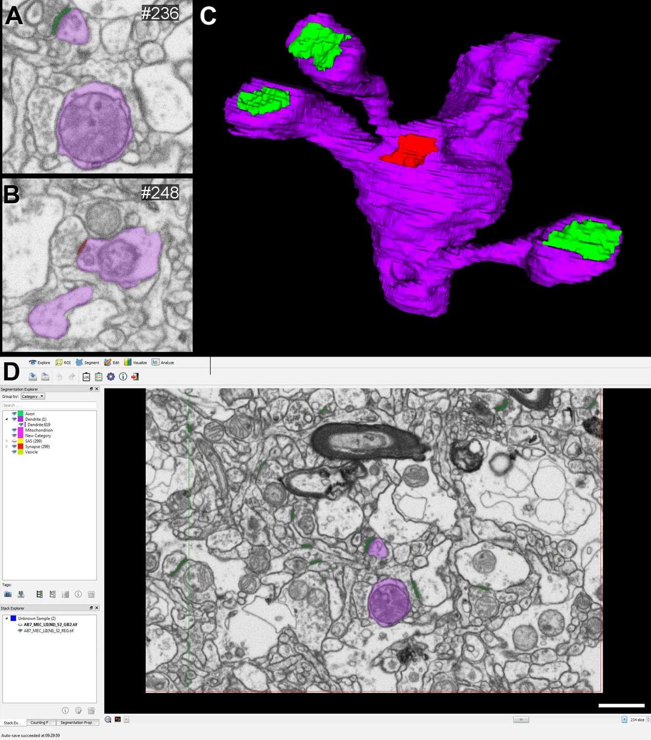
3D reconstruction of a dendritic segment from focused ion beam FIB/SEM serial images.
(A, B) Serial images showing a dendritic segment partially reconstructed (in purple). An asymmetric synapse (in A) on a dendritic spine head and a symmetric synapse (in B) on a shaft are indicated in green and red, respectively. (C) 3D reconstruction of the dendritic segment indicated in (A) and (B). Three dendritic spines receiving asymmetric synapses can be observed, along with a symmetric synapse formed on the dendritic shaft. (D) Snapshot of EspINA software interface displaying the reconstructed dendritic segment. Scale bar (in C): 500 nm in (A, B), 370 nm in (C) and 900 in (D).
Figure 13—video 1
Visualization of the reconstructed dendritic segment of Figure 13 using EspINA software.
Tables
Table 1
Accumulated data obtained from the ultrastructural analysis of neuropil from layers I, II-is, II-ni, III, Va/b, Vc, and VI of the MEC.
Data in parentheses are not corrected for shrinkage. AS, asymmetric synapses; CF, counting frame; SS, symmetric synapses; SAS, synaptic apposition surface.
| Layer | No. of AS | No. of SS | No. all synapses | % AS (mean) | % SS (mean) | CF volume (μm3) | No. AS/µm3 (mean ± SD) | No. SS/µm3 (mean ± SD) | No. all synapses/µm3 (mean ± SD) | Area of SAS AS (nm2; mean ± SE) | Area of SAS SS (nm2; mean ± SE) | Intersynaptic distance (nm; mean ± SD) |
|---|---|---|---|---|---|---|---|---|---|---|---|---|
| I | 1265 | 80 | 1345 | 94 | 6 | 2585 (3265) | 0.44 ± 0.06 (0.39 ± 0.05) | 0.03 ± 0.01 (0.03 ± 0.01) | 0.47 ± 0.06 (0.41 ± 0.05) | 105,906 ± 3583 (98,493 ± 3332) | 53,367 ± 2337 (49,631 ± 2173) | 850 ± 64 (824 ± 62) |
| II-is | 1255 | 100 | 1355 | 92.6 | 7.4 | 2949 (3142) | 0.38 ± 0.04 (0.40 ± 0.05) | 0.03 ± 0.01 (0.03 ± 0.01) | 0.42 ± 0.04 (0.43 ± 0.05) | 118,070 ± 6221 (109,805 ± 5786) | 67,492 ± 5135 (62,768 ± 4776) | 876 ± 68 (850 ± 66) |
| II-ni | 1290 | 97 | 1387 | 93.1 | 6.9 | 2820 (3018) | 0.41 ± 0.05 (0.43 ± 0.06) | 0.03 ± 0.01 (0.03 ± 0.01) | 0.44 ± 0.06 (0.46 ± 0.06) | 118,550 ± 5606 (110,251 ± 5214) | 73,141 ± 6195 (68,022 ± 5762) | 845 ± 52 (819 ± 51) |
| III | 1216 | 74 | 1290 | 94.1 | 5.9 | 2901 (3013) | 0.38 ± 0.07 (0.40 ± 0.08) | 0.02 ± 0.01 (0.02 ± 0.01) | 0.40 ± 0.08 (0.43 ± 0.07) | 130,268 ± 5734 (121,150 ± 5333) | 74,248 ± 9112 (69,051 ± 8474) | 882 ± 90 (856 ± 87) |
| Va/b | 1145 | 50 | 1195 | 95.8 | 4.2 | 3017 (3131) | 0.34 ± 0.05 (0.36 ± 0.06) | 0.01 ± 0.005 (0.01 ± 0.005) | 0.35 ± 0.05 (0.38 ± 0.06) | 136,111 ± 5571 (126,583 ± 5181) | 74,698 ± 7914 (69,469 ± 7360) | 899 ± 48 (871 ± 46) |
| Vc | 1257 | 87 | 1344 | 93.5 | 6.5 | 2983 (3118) | 0.38 ± 0.08 (0.40 ± 0.9) | 0.03 ± 0.01 (0.03 ± 0.01) | 0.41 ± 0.08 (0.43 ± 0.09) | 126,298 ± 5071 (117,457 ± 4716) | 87,377 ± 4716 (81,377 ± 4408) | 865 ± 66 (840 ± 64) |
| VI | 1177 | 53 | 1230 | 95.6 | 4.4 | 3112 (3239) | 0.34 ± 0.05 (0.37 ± 0.06) | 0.02 ± 0.01 (0.02 ± 0.01) | 0.36 ± 0.05 (0.38 ± 0.06) | 99,489 ± 6438 (92,525 ± 5987) | 69,365 ± 10,685 (64,509 ± 9937) | 851 ± 77 (826 ± 75) |
| I-VI | 8605 | 541 | 9146 | 94.1 | 5.9 | 20,367 (21,926) | 0.38 ± 0.03 (0.39 ± 0.02) | 0.02 ± 0.01 (0.02 ± 0.01) | 0.41 ± 0.04 (0.42 ± 0.03) | 119,242 ± 2512 (110,895 ± 2336) | 71,384 ± 2806 (66,387 ± 2610) | 867 ± 67 (841 ± 65) |
Table 2
Coefficient of variation (CV) of the analyzed synaptic parameters in each MEC layer between individuals.
CV was calculated by dividing the SD by the mean and multiplying by 100 for each of the synaptic parameters analyzed.
AS, asymmetric synapses; SAS, synaptic apposition surface.
| Layer | Synaptic density | Proportion of AS | AS SAS area | Proportion of macular AS | Proportion of AS on spines |
|---|---|---|---|---|---|
| I | 5.4 | 1.0 | 3.3 | 4.0 | 5.1 |
| II-is | 7.0 | 0.8 | 17.3 | 7.0 | 11.4 |
| II-ni | 1.3 | 3.3 | 10.7 | 6.5 | 10.3 |
| III | 4.3 | 0.4 | 5.4 | 3.9 | 1.1 |
| Va/b | 9.9 | 0.3 | 15.5 | 5.7 | 13.5 |
| Vc | 11.7 | 1.9 | 2.4 | 4.6 | 7.5 |
| VI | 11.7 | 1.7 | 19.6 | 3.8 | 5.0 |
Additional files
-
Supplementary file 1
Supplementary tables.
(a) Light microscopy data: volume fraction occupied by cortical elements in layers I, II-is, II-ni, III, Va/b, Vc, and VI of the MEC. Vc: volume fraction occupied by cells bodies; Vbv: volume fraction occupied by blood vessels; Vn: volume fraction occupied by neuropil. (b) Light microscopy data: volume fraction occupied by cortical elements in layers I, II-is, II-ni, III, Va/b, Vc, and VI of the MEC, for individual cases. Vc: volume fraction occupied by cells bodies; Vbv: volume fraction occupied by blood vessels; Vn: volume fraction occupied by neuropil. (c) Summary of the stack details obtained from the multiple sampling from all layers of MEC. Three stacks of images were acquired in each MEC layer, per case (nine stacks of images in total per layer). The last row shows the sum of all the MEC layers from all cases. (d) Accumulated data acquired from the ultrastructural analysis of neuropil from layers I, II-is, II-ni, III, Va/b, Vc, and VI of the MEC for individual cases. Data in parentheses are not corrected for shrinkage. AS: asymmetric synapses; CF: counting frame; SS: symmetric synapses. (e) Number of synaptic SAS analyzed (n), the location (µ), and scale (σ) of the best-fit log-normal distributions in the six cortical layers. AS: asymmetric synapses; SAS: synaptic apposition surface; SS: symmetric synapses. (f) Proportion of the different shapes of synaptic junctions in MEC layers. Data in parentheses refer to absolute numbers of synapses. (g) Proportion of the different shapes of synaptic junctions in MEC layers for individual cases. Data in parentheses refer to absolute numbers of synapses. (h) SAS area of asymmetric (AS) and symmetric (SS) synapses for each synaptic shape in each MEC layer. Data in parentheses are not corrected for shrinkage. Values (in nm2) are expressed as mean ± SE. (i) SAS area of asymmetric (AS) and symmetric (SS) synapses for each synaptic shape, in each MEC layer, per individual case. Data in parentheses are not corrected for shrinkage. Values (in nm2) are expressed as mean ± SE. (j) Proportion of the different postsynaptic targets in MEC layers. Synapses established on spine head include both complete and incomplete spines. Data in parentheses refer to the absolute number of synapses found in each layer. (k) Proportion of the postsynaptic targets of synaptic junctions in MEC layers, for individual cases. Total synapses on spine heads are calculated as the sum of ‘Complete Spine Heads’ and ‘Incomplete Spine Heads’ columns. Data in parentheses refer to the absolute numbers of synapses. (l) SAS area of asymmetric (AS) and symmetric (SS) synapses regarding the postsynaptic target in each MEC layer. Data in parentheses are not corrected for shrinkage. Values (in nm2) are expressed as mean ± SE. (m) SAS area of asymmetric (AS) and symmetric (SS) synapses according to the postsynaptic target in each MEC layer, per individual case. Data in parentheses are not corrected for shrinkage. Values (in nm2) are expressed as mean ± SE. (n) Coefficient of variation of the analyzed synaptic parameters in each MEC layer between the stack of images. AS: asymmetric synapses; CV: coefficient of variation; SAS: synaptic apposition surface. (o) Data on postsynaptic targets in different species, regions, and cortical layers. EC: entorhinal cortex; F: female; FIB/SEM: focused ion beam-SEM; M: male; MEC: medial entorhinal cortex; TCE: transentorhinal Cortex; TEM: transmission electron microscopy. Age refers to years, except otherwise indicated. *No classification of the type of synapses (AS:SS) were performed. **Only axospinous synapses (established on dendritic spine heads and necks) and axodendritic synapses (formed on dendritic shafts) are indicated. ***No distinction between spiny and aspiny shafts were made. (p) Clinical and neuropsychological information from the cases analyzed.
- https://cdn.elifesciences.org/articles/96144/elife-96144-supp1-v2.docx
-
Supplementary file 2
Spreadsheet containing the spatial extents of individual stacks of images, detailed per case, and layer.
Original dimensions (x, y, z), original volumes, counting frame (CF) dimensions, and CF volume are provided.
- https://cdn.elifesciences.org/articles/96144/elife-96144-supp2-v2.xlsx
-
Supplementary file 3
Spreadsheet containing Kruskal–Wallis and Dunn’s tests p-values of the interindividual variability analysis, organized in TABS as follows.
The criterion for statistical significance was considered to be met if p<0.05 (indicated in the spreadsheet as *) or p<0.01 (**).
- https://cdn.elifesciences.org/articles/96144/elife-96144-supp3-v2.xlsx
-
Supplementary file 4
Spreadsheet containing the complete raw dataset organized in TABS as follows: RAW DATA SYNAPSES: each row corresponds to each analyzed synapse and contains its characteristics, SAS area corrected for tissue shrinkage and SAS area provided by EspINA.
RAW DATA DENSITIES: each row corresponds to each analyzed stack of images and contains the number of synapses per type, the volume of the counting frame, the volume of the counting frame corrected for tissue shrinkage and artifacts, and the calculated synaptic density per type and total.
SIZE: mean SAS area, SE, and number of synapses calculated per stack of images, per synaptic type and layer. SHAPE: number of synapses, mean SAS area and SE per synaptic shape, calculated per stack of images, synaptic type, and layer.
POSTSYNAPTIC: number of synapses, mean SAS area and SE per postsynaptic target, calculated per stack of images, synaptic type, and layer.
- https://cdn.elifesciences.org/articles/96144/elife-96144-supp4-v2.xlsx
-
MDAR checklist
- https://cdn.elifesciences.org/articles/96144/elife-96144-mdarchecklist1-v2.docx
Download links
A two-part list of links to download the article, or parts of the article, in various formats.
Downloads (link to download the article as PDF)
Open citations (links to open the citations from this article in various online reference manager services)
Cite this article (links to download the citations from this article in formats compatible with various reference manager tools)
Volume electron microscopy reveals unique laminar synaptic characteristics in the human entorhinal cortex
eLife 14:e96144.
https://doi.org/10.7554/eLife.96144


