How competition governs whether moderate or aggressive treatment minimizes antibiotic resistance
- Imperial College London, United Kingdom
- Yale University, United States
Figures
Figure 1
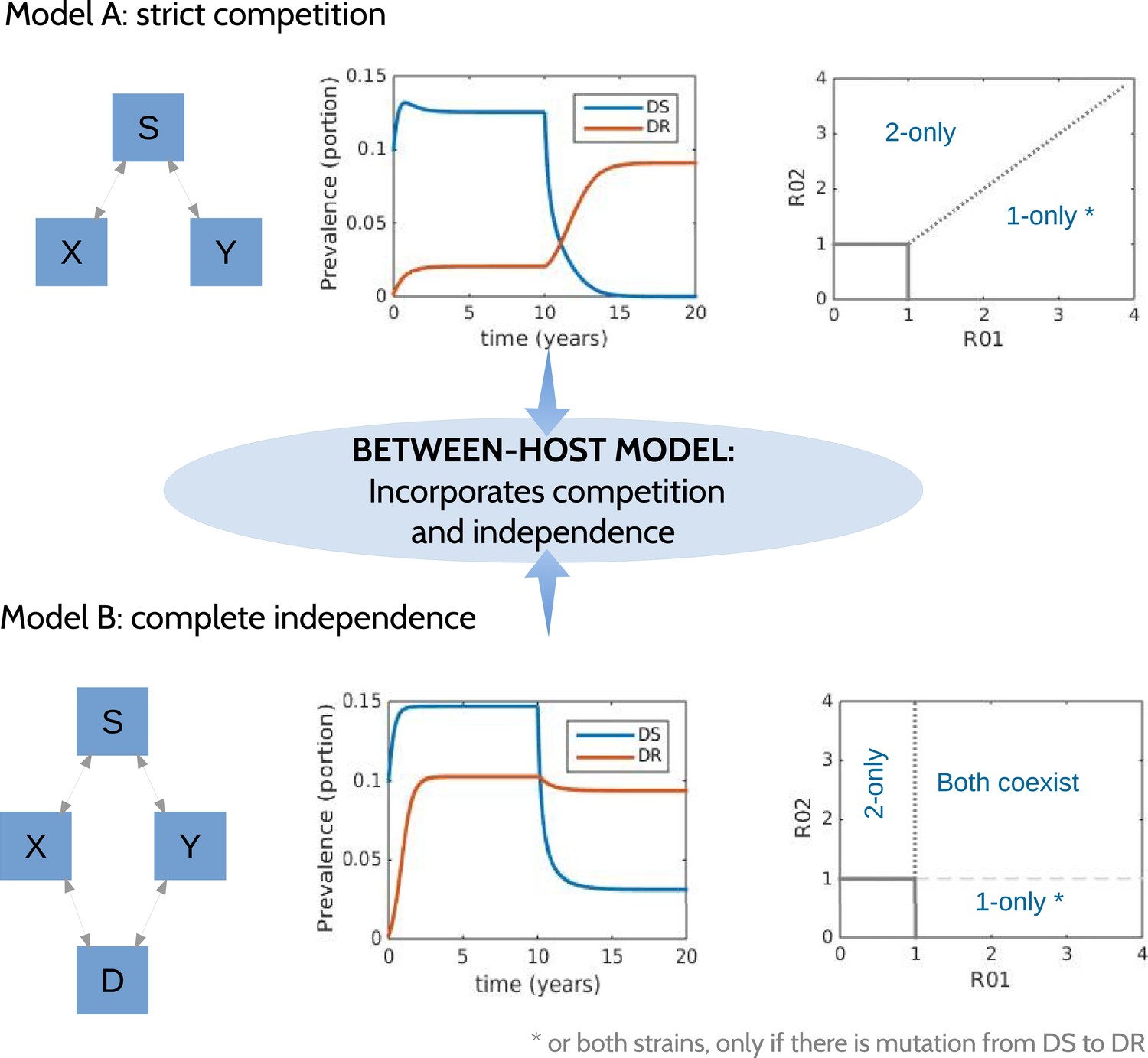
Models at the two ends of the competition independence spectrum (between hosts).
In the competing model (top row), decreasing the DS strain (X) paves the way for an increase in resistance (Y) by removing the DR strain's competitor, despite the fact that decreasing DS also removes a source of resistance. The bifurcation analysis illustrates competitive exclusion: whichever strain has the higher R0 excludes the other. In both cases, some resistance is present when the sensitive strain is present, due to acquisition of resistance, for example, through mutation. Consequently, the ‘1-only’ region of the plot has some strain 2 at very low prevalence. In contrast, if the strains are not competing (bottom row), including not competing for hosts, hosts must be able to harbor both infections (duals, D). In this case, reducing DS reduces DR by reducing a source of resistance. The bifurcation plot where strains are independent illustrates that strain 1 is present if R01 > 1, strain 2 is present if R02 > 1 and both are present if they are both >1. Our between-host model incorporates competition and independence, parameterized by a ‘similarity coefficient’ that smoothly moves from one to the other (see Appendix 1 for details).
Figure 2
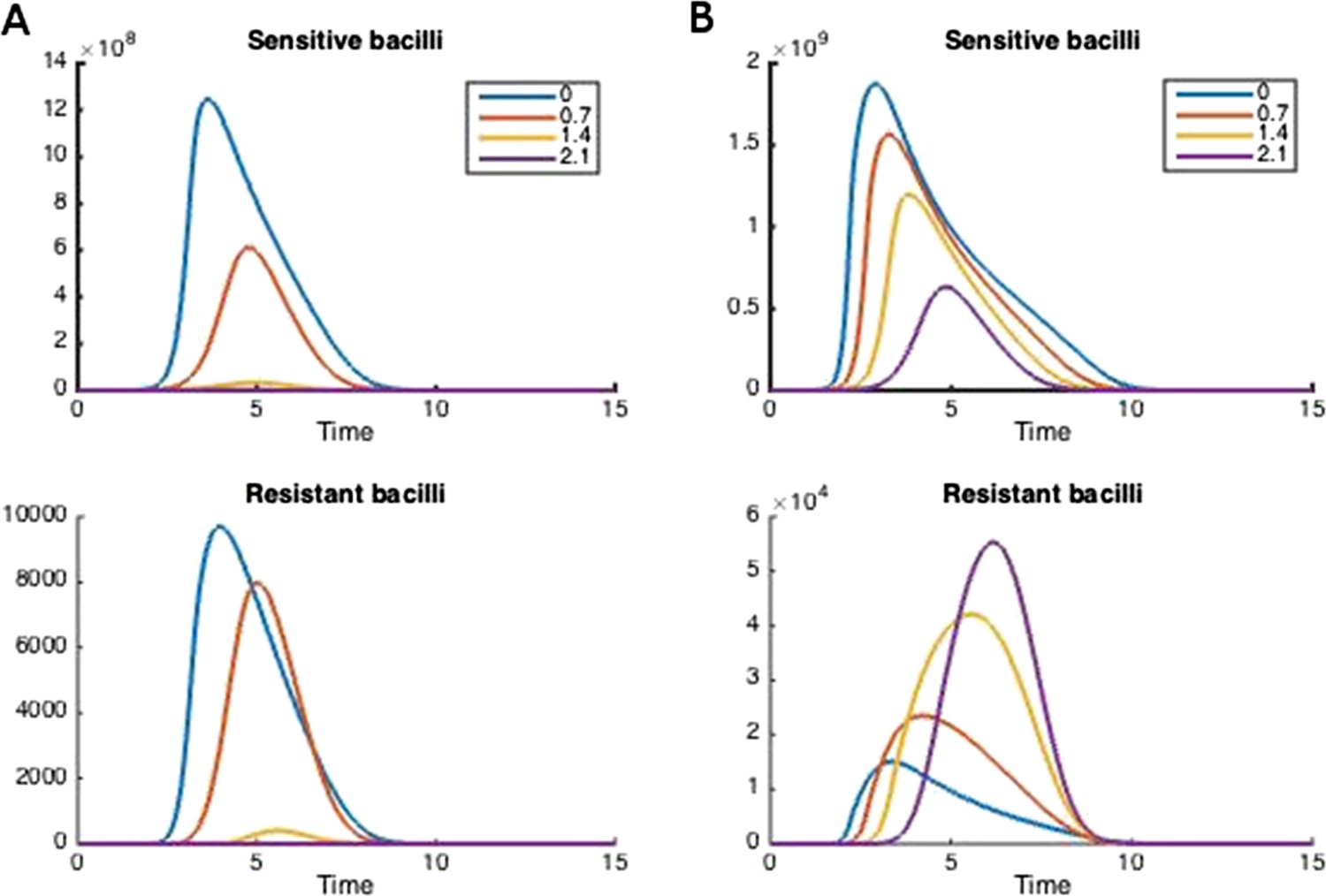
How treatment changes the trajectory of the in-host model.
Parameters are (A) Λs = 0.5, Λr = 0.45, mR = 2.8 and (B) Λs = 0.6, Λr = 0.53, mR = 3.4. Other parameters are k = 48, kp = 2.2e−6, ki = 7.2e−4, μ = 4e−7, α = 0.018, σi = 1000, σp = 10000, γp = 0.001, and the remainder are as in Table 1.
Figure 3
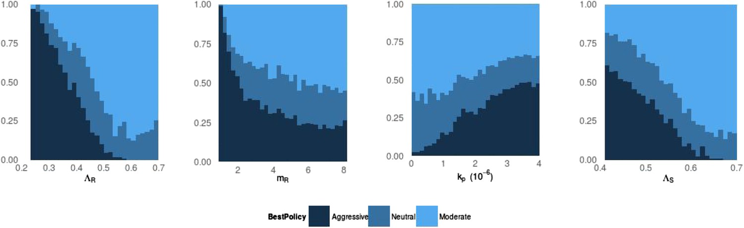
Frequency of best policies over key parameters.
An aggressive policy (dark blue) is deemed best if the Spearman correlation S between treatment and resistance is S < −0.7, moderate (light blue) is deemed best if S > 0.7 and the classification is neutral (medium blue) otherwise. When the DR strain has a lower growth rate (LamR), an aggressive policy is more likely best because more of the DR strain's population arises through resistance acquisition from the DS population. In this case, reducing the DS strain also reduces DR. Conversely, when ΛR (LamR) is high the DR strain is a more robust competitor and a moderate policy is more frequently best. Similarly, when the DR strain has a low MIC (mR), it is a less robust competitor. In this case, an aggressive policy is more frequently best than when mR is high (second panel). The third panel shows that when the immune system is strong (high kp), an aggressive policy is more frequently best, because again more of the DR population increases are driven by acquisition from DS, due to immune suppression of DR growth. A plot with η on the horizontal axis is very similar to this one. Finally, the right plot shows that when the DS growth rate (LamS) is low, an aggressive strategy is more often best to minimize resistance; this depends on the ability of therapy to prevent the emergence of resistance.
Figure 4
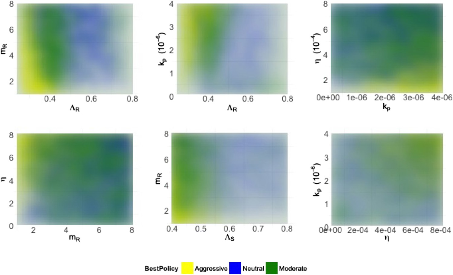
Heatmaps illustrating how best policies depend on key combinations of parameters.
Color indicates the policy that minimizes resistance. Yellow: aggressive; green: neutral; blue: moderate. When the growth rate ΛR (LamR) is high, a moderate policy is more frequently best, but a strong immune system (high kp) can compensate by reducing DR growth. When the DR strain is a strong competitor, a moderate policy is frequently best; this can be achieved by either a high ΛR or a high DR MIC (mR) (top left). Either a high kp or a high η can compensate (bottom right), reducing the growth potential of the DR strain and leading to either a neutral outcome or an aggressive policy being best.
Figure 5

Trajectories of the between-host model under varying treatment.
Treatment is introduced at 5 years. (Left) Parameters are βx = 1.5, βy = 1.04, c = 0.05, r = 0, μ = 0.001. (Middle) Parameters are βx = 2, βy = 1.1, c = 0.3, r = 0.05, μ = 0.0001. (Right) Invasion analysis (bifurcation) plot. The plot shows regions of stability of the disease-free equilibrium (both R0 values less than one), the DR-only equilibrium (top left region), and the equilibrium with both (primarily DS, with low-level DR due to acquisition). The diagonal lines show the boundary at which the DR-only equilibrium loses stability. Lines move to the right as the similarity coefficient increases from 0 (light blue vertical line) to 1 (pink). When it reaches 1, the line is R01 = R02.
Figure 6
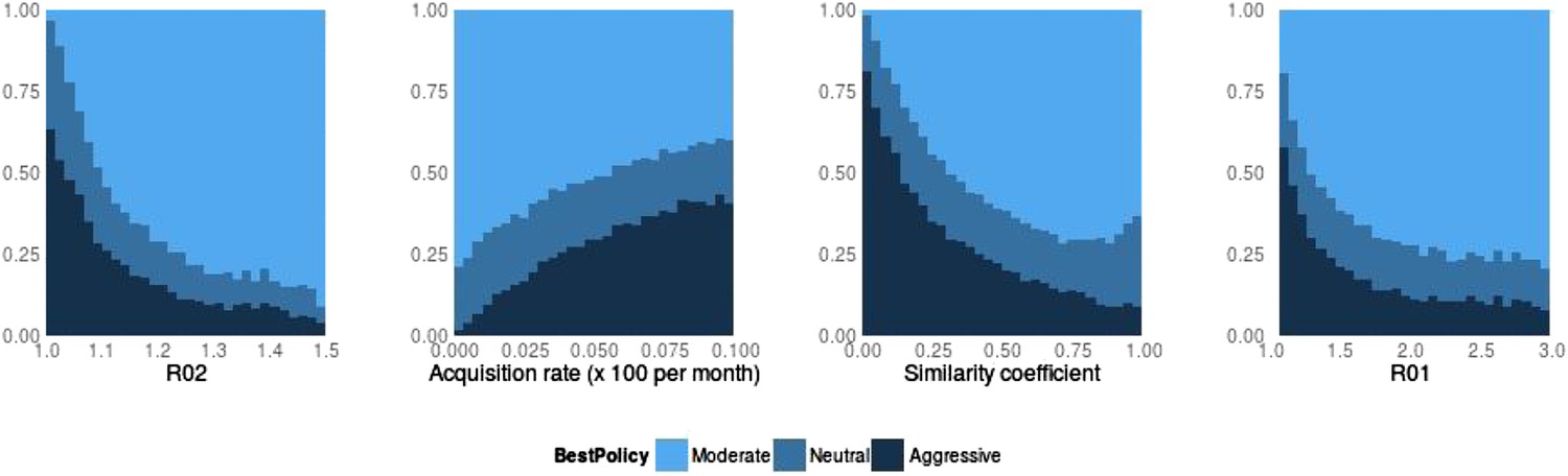
Best policy over parameters in the population-level model.
Light blue corresponds to Spearman correlation greater than 0.7, dark corresponds to less than −0.7 and mid-range blue corresponds to all values in between. An aggressive policy is best when the DR strain is relatively unfit (low R0 value; left panel). When the acquisition rate is high, treatment-driven reductions in DS decrease the DR prevalence (second panel). When the two strains are more independent (low similarity coefficient), competition is reduced, so that reductions in the DS strain do not much benefit the DR strain, leading to the aggressive policy being preferred (third panel). When R01 is high, a moderate outcome results, because inter-strain competition is more effective. Vertical axes (‘count’) are the fraction of simulations in each category.
Figure 7
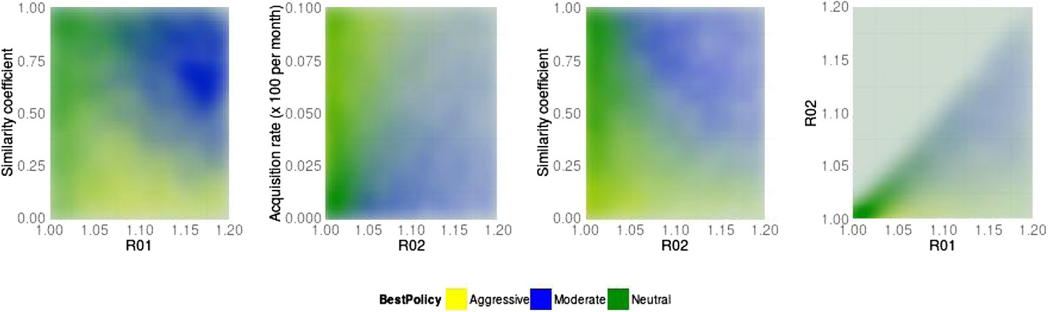
Best policy over parameter combinations in the population-level model.
A moderate-is-best (blue) outcome occurs when R01 and the similarity coefficient are high, because the strains are competing (left panel). When the DR strain is relatively unfit (low R02), an aggressive policy is likely best (second and third panels); we restricted R02 to be lower for the DR strain than the DS one. A high rate of acquisition can counter-balance a low R02 (second panel). When the strains are more independent (low similarity coefficient), an aggressive policy is more often best even over a much wider range of R02 (third panel).
Appendix figure 1

Heatmaps illustrating whether aggressive therapy (yellow), moderate therapy (blue) or neither, conclusively (neutral; green) minimize resistance.
(Top set of panels) Pre-existing resistance means that the ‘moderate is best’ conclusion is spread out more widely over the parameter space; the DR strain does not benefit as much from DS growth. (Bottom set of panels) Without pre-existing resistance, there is more clear separation between the parameter regimes. Overall, the results are the same as in the main text: a moderate outcome is driven by high effective competition between strains, meaning a higher ΛR, mR and lower values of immune parameters kp and η (eta).
Appendix figure 2
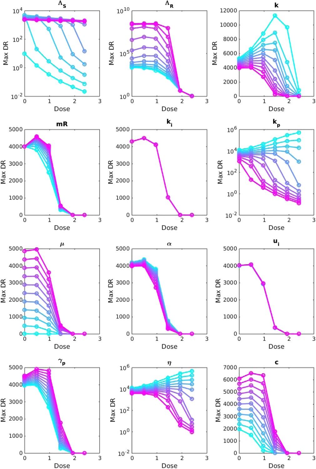
Sensitivity analysis, varying one parameter at a time.
For each value of each parameter, the dosage was increased from 0 to 2.5 μg/ml per day, and the maximum number of DR bacilli during the infection was recorded. The baseline values of the parameters (when they were not varied) are: Λs = 0.5, Λr = 0.45, mR = 2.8 and the remainder are as in Table 1.
Appendix figure 3
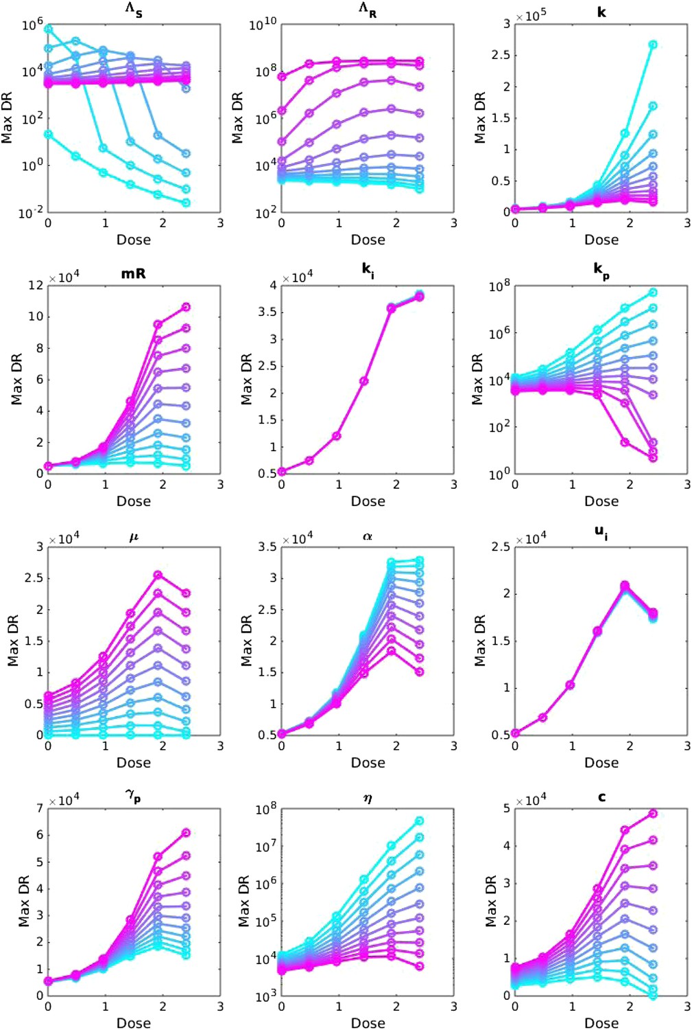
Sensitivity analysis, varying one parameter at a time.
For each value of each parameter, the dosage was increased from LOW to HIGH, and the maximum number of DR bacilli during the infection was recorded. The baseline values of the parameters (when they were not varied) are: Λs = 0.6, Λr = 0.53, mR = 3.4. Other parameters are k = 48, kp = 2.2e−6, ki = 7.2e−4, μ = 4e−7, α = 0.018, σi = 1000, σp = 10000, γp = 0.001 and the rest as in Table 1. The approach is the same as that in Appendix figure 2, except that the baseline set of parameters is different.
Appendix figure 4
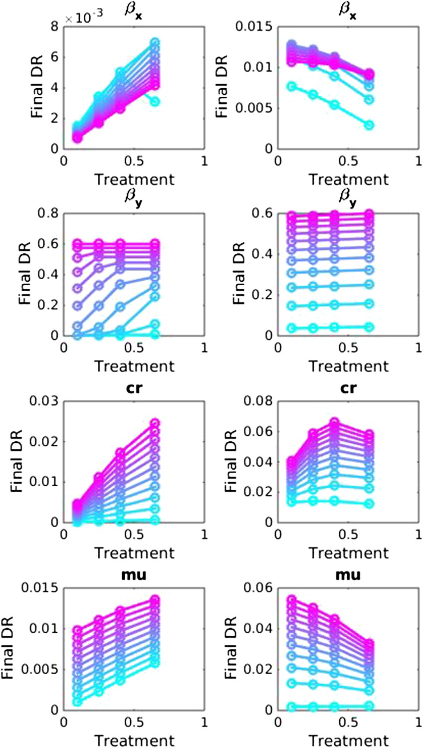
Sensitivity analysis, varying one parameter at a time in the between-host model over the ranges listed in Table 1.
Left side: baseline parameter values are βx = 1.5, βy = 1.04, c = 0.05, r = 0, μ = 0.001. Right side: baseline values are βx = 2, βy = 1.1, c = 0.3, r = 0.05, μ = 0.0001.
Appendix figure 5
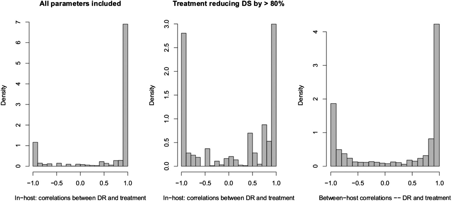
Spearman correlations between treatment level and maximum resistance in both models.
(Left) In-host model. Left panel shows all parameters. Right panel shows only those for which treatment succeeds. The difference is that where treatment does not succeed, it drives resistance. (Right) Population-level model.
Appendix figure 6
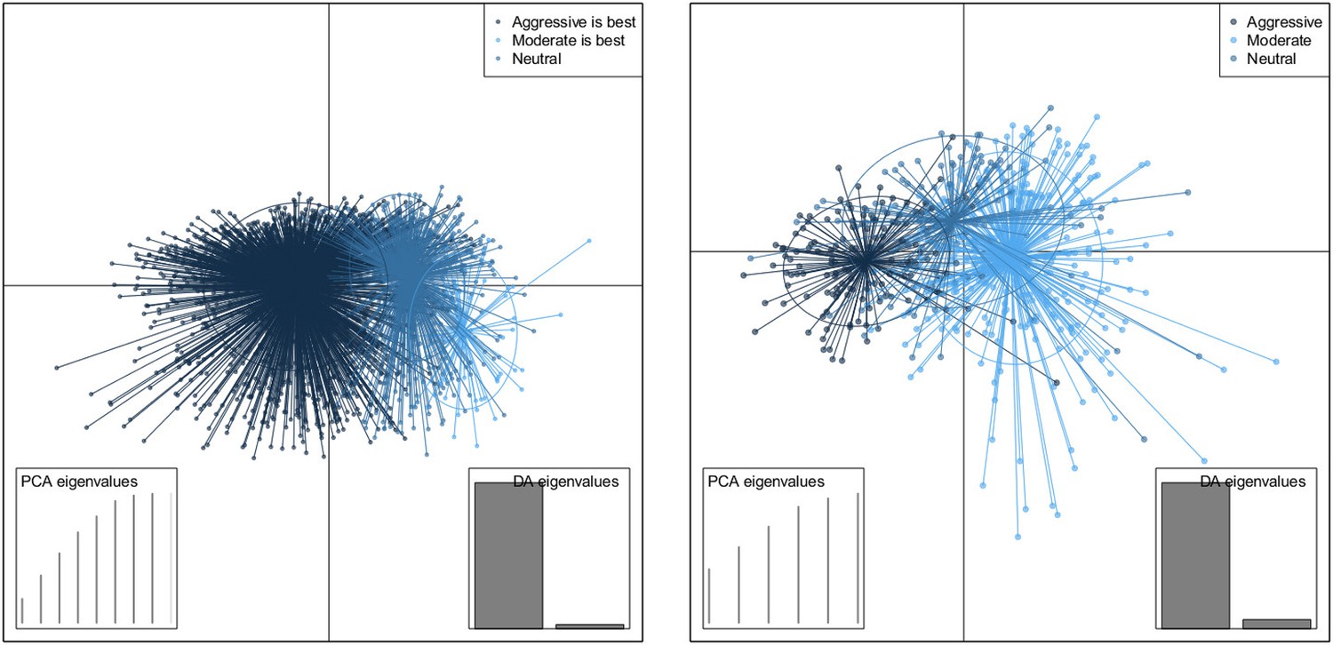
DAPC scatterplot for the within-host model.
The x-axis is a linear combination of parameters corresponding to the primary DAPC discriminant function, and the y-axis corresponds to the second. Accordingly, the groups are plotted by their positions on the first two DAPC axes. The relative portions of the variance that these axes capture is illustrated in the DACP eigenvalue plot (bottom right corner). Almost all of the difference between the groups is captured by the x-axis (high gray bar in the bottom left plot, compared to a low gray bar for the variation captured by the second axis). The PCA eigenvalues plot in the bottom right shows the portion of variance retained when keeping k PCA axes. In both models, the neutral group, in which treatment was not strongly correlated with the level of resistance in either direction, lies directly between the aggressive and moderate groups.
Appendix figure 7
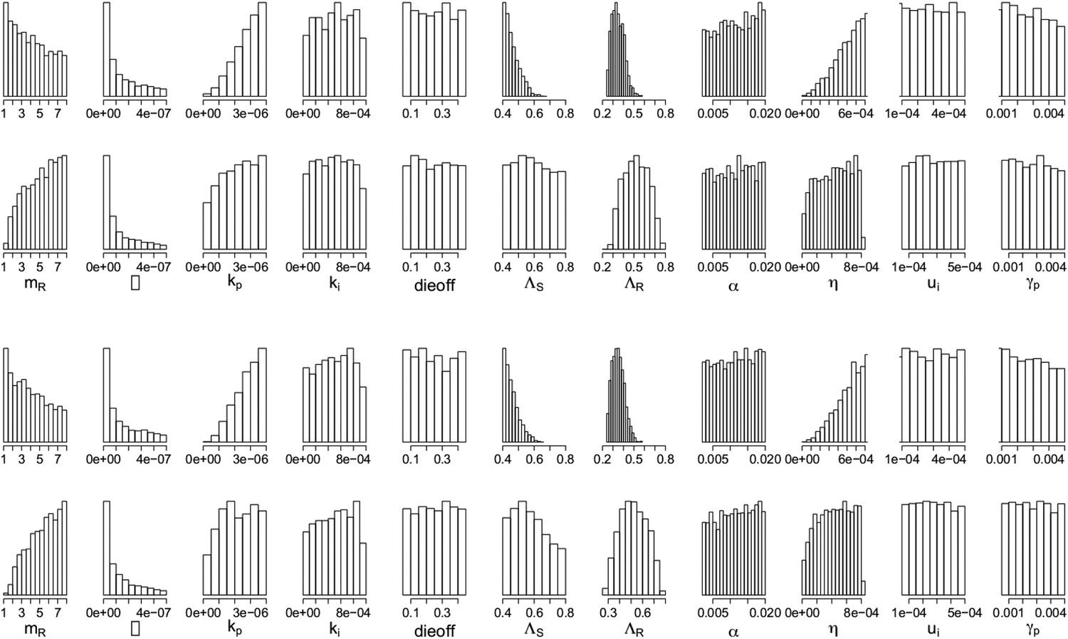
Parameters from the two regimes: (a) with the lysis term and (b) without it.
In each set, the top row shows the parameters under which resistance decreases with increasing dosage, and the bottom row shows those for which resistance increases with increasing dosage. The relationships between the two outcomes (treatment increasing or decreasing resistance) are unaffected by whether the lysis term is included. Removing the term is akin to including lysis in the equation for the resource usage, but with an e coefficient of 0; a more general model could include this with a coefficient el < e which would model the fact that resource consumption and release could happen with different efficiencies. Though we do not know what an appropriate choice for el would be, the results with el = 0 (bottom set of histograms) are the same as those with el = e (original model; top set of histograms).
Appendix figure 8
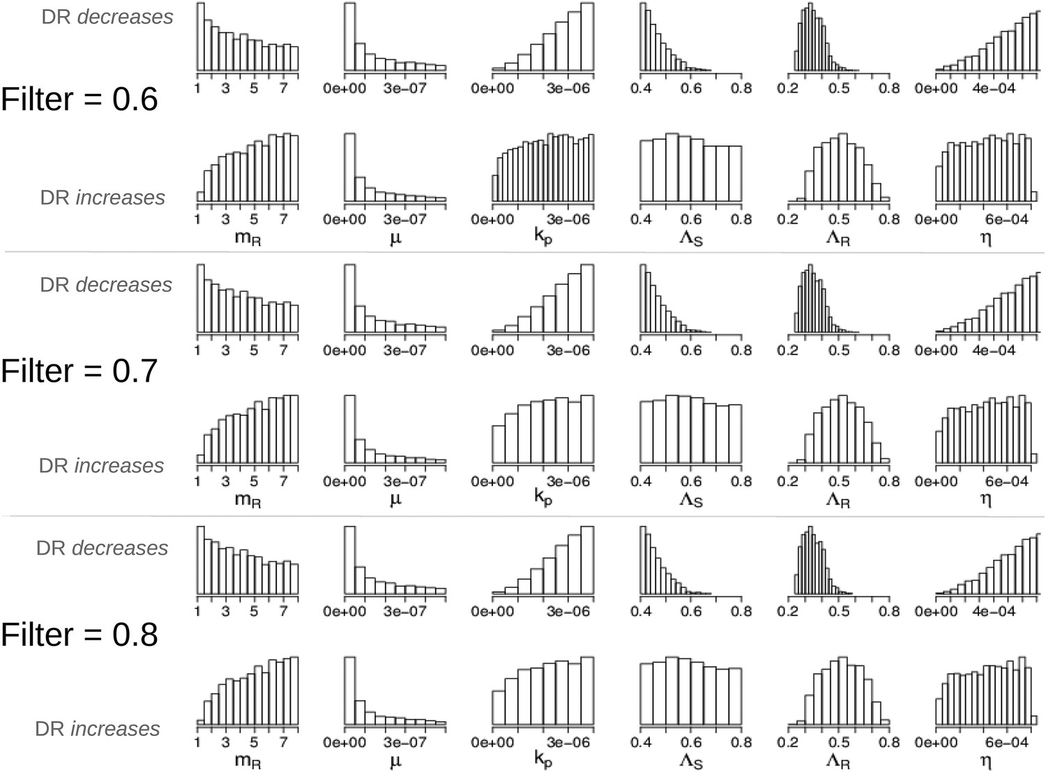
Parameters in the two modes showing that the filter defining ‘effective treatment’ does not change the relationships between parameters and whether treatment increases or decreases resistance.
We have shown only the parameters whose distributions are different in the two modes (compare to Appendix figure 7).
Appendix figure 9
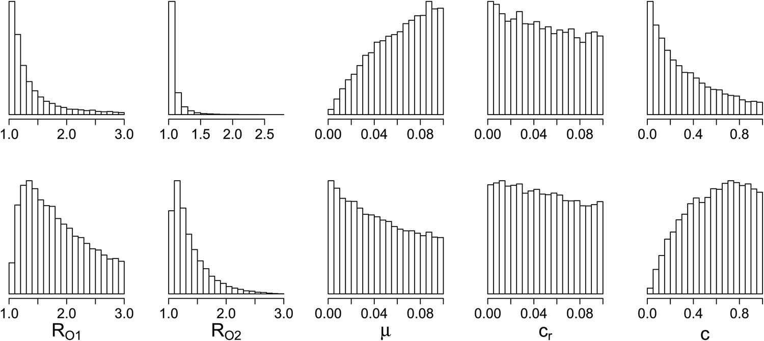
Parameters where the two contrasting policies work best in the population level model.
Top row: treatment decreases resistance. Bottom row: treatment increases resistance.
Appendix figure 10
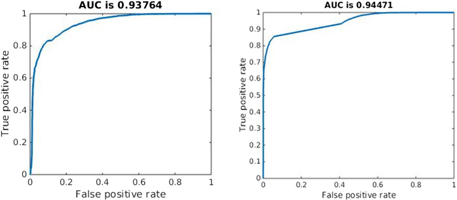
Quality of classification using the instantaneous measure of effective competition to classify a parameter set according to whether treatment will increase or decrease resistance.
A random classifier has an AUC of 0.5. We used the sign of the Spearman correlation between treatment and resistance as the ‘true’ classification (competing if treatment increases resistance), and the value of our effective competition quantity as the ‘scores’. Curves were created using the perfcurve function in matlab.
Tables
Table 1
Parameters and ranges
| Symbol | Description | Range | Unit |
|---|---|---|---|
| Within-host model | |||
| Λs | Max growth rate (DS) | 0.4–0.8 | hr−1 |
| Λr | Max growth rate (DR) | (0.6–1) × Λs | hr−1 |
| k | Hill coeffient in bacterial growth | 0.5–50.5 | μg/ml |
| us, ur | Death rates DS, DR | 0.2 | hr−1 |
| mS | MIC (DS) | 1 | μg/ml |
| mR | MIC (DR) | 1–8 | μg/ml |
| kp | Rate of innate immune clearance | 10−7 − 10−5 | hr−1 |
| ki | Rate of adaptive immune clearance | 10−5 − 10−3 | hr−1 |
| μ | Rate of DR mutation | 5 × 10⁻⁹ − 5 × 10⁻⁷ | #/division |
| α | Recruitment of adaptive immunity | 0.002–0.02 | hr−1 |
| σi, σp | Hill parameter in I, P dynamics | 1000, 10,000 | cells/ml |
| ui | Loss rate of I | 5 × 10⁻⁵ − 5 × 10⁻⁴ | hr−1 |
| γ | Loss rate of P | 5 × 10⁻⁴ − 5 × 10⁻³ | hr−1 |
| η | Recruitment of innate immunity | 10−5 − 9 × 10⁻⁴ | hr−1 |
| w | Washout rate | 0.2 | hr−1 |
| CR | Resource reservoir concentration | 300–700 | μg/ml |
| e | Use of resource per unit growth | 5 × 10⁻⁷ | μg/cell |
| Ain | Antibiotic treatment | 0–2.5 | μg/(ml × 24 hr) |
| d | Loss rate of antibiotic | 0.1 | hr−1 |
| Between-host model | |||
| βx | Transmission parameter (DS) | 1–4 | months−1 |
| βy | Transmission parameter (DR) | 1 − βx | months−1 |
| κ | Partial immunity coefficient | 1 | none |
| κt | Treatment protection from DS | 1 − 0.3T | none |
| c | Similarity coefficient | 0–1 | none |
| u | DS clearance without treatment | − | months−1 |
| uy | DR clearance | βy/R01 − βy | months−1 |
| T | Intensity of treatment | 0–1 | none |
| r | Release of DS through treatment | 0–0.1 | months−1 |
| umax | Max clearance DS under treatment | 1.05 βx | months−1 |
-
Ranges are indicated with a − separating lower and upper values. Where a single value is given the parameter was fixed. Within-host parameter ranges contain the values used in Ankomah and Levin (2014). The relative growth of the resistant and sensitive strains (without treatment) can be modified either through k or Λ. We have chosen to vary the Λ parameters as the effect on relative fitness is linear. In the between-host model the value of u was chosen such that the DS strain has a basic reproductive number in Bonhoeffer et al. (1997) and Ankomah and Levin (2014). Similarly, uy was chosen so that R02 ranges from 1 to R01, to ensure that the DR strain has a smaller maximum growth rate than the DS strain.
Download links
A two-part list of links to download the article, or parts of the article, in various formats.
Downloads (link to download the article as PDF)
Open citations (links to open the citations from this article in various online reference manager services)
Cite this article (links to download the citations from this article in formats compatible with various reference manager tools)
How competition governs whether moderate or aggressive treatment minimizes antibiotic resistance
eLife 4:e10559.
https://doi.org/10.7554/eLife.10559


