Figures and data in Self-blinding citizen science to explore psychedelic microdosing

Figures
Tables
Additional files

8 figures, 3 tables and 9 additional files

Figures

Figure 1

Download asset Open asset

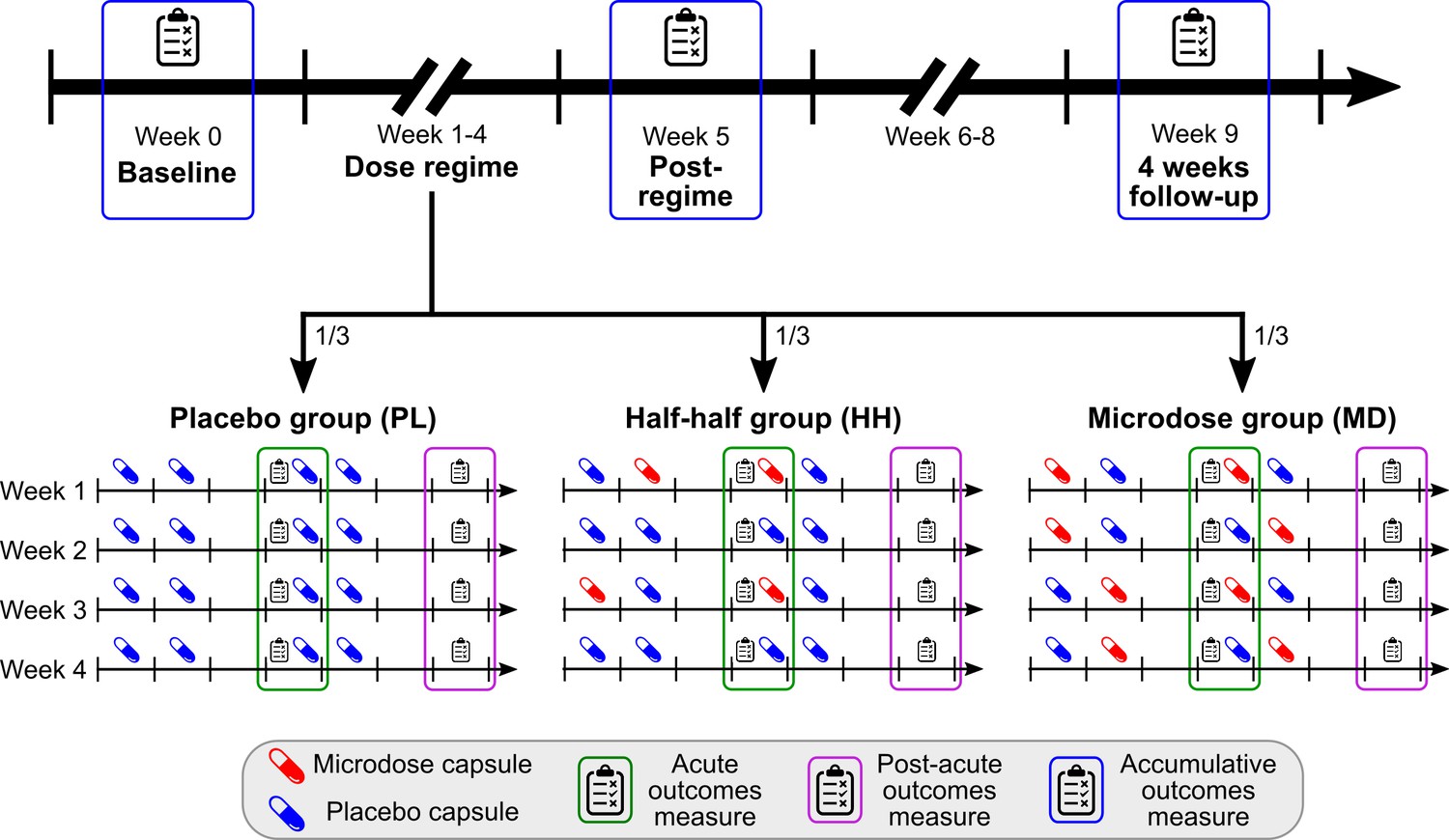
Timeline and outcomes.

Top horizontal arrow shows the experimental timeline and the three timepoints associated with accumulative outcomes (blue frame). 1/3 of the participants were randomly assigned to one of the three groups, where the groups differ in the number of placebo/microdose weeks during the dose-regime: 4/0 for PL, 2/2 for HH, and 0/4 for the MD group. Note that even for microdose weeks, placebo capsules are mixed into the schedule, for example, weeks 1 and 3 for the HH group are microdose weeks. Acute measures (green frames) were taken on Thursdays, while the potential microdose was still active. Post-acute measures (purple frame) were administered on Sundays, when no capsule was taken, these outcomes test the weekly effects of microdosing. For a list of measures administered at each timepoint, see Table 1.

Figure 2

Download asset Open asset

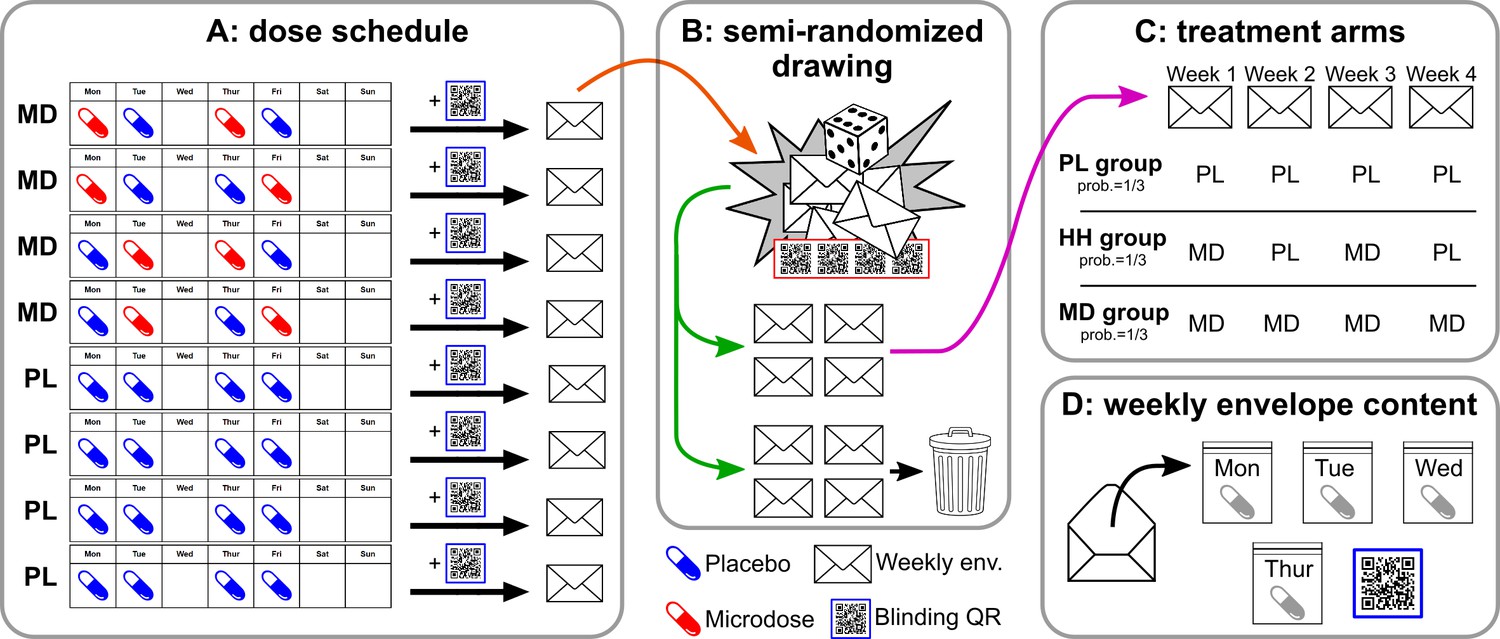
Overview of the self-blinding setup.

First, capsules are prepared: microdoses are put into opaque gel capsules, while empty capsules are used as placebos. Next, weekly sets of capsules are assembled according to the dose schedule (A; no capsules taken on Wed., Sat., and Sun.). Then, capsules are placed inside zip bags with a printed day label (Monday, Tuesday, etc.; zip bags and day labels not shown on figure). Next, each weekly set and a unique QR code are placed inside envelopes. Eight such weekly envelopes are prepared, four of which correspond to microdose weeks (MD) and four that corresponds to placebo weeks (PL). The eight envelopes are used in a semi-random drawing process (orange arrow, B), which involves another set of QR codes and random number generation, see Appendix 1—figure 1 for details. The drawing selects four envelopes, corresponding to the 4 weeks of the dose period, while the remaining four are discarded (green arrow). The drawing is constrained such that only the three combinations of PL/MD weeks are possible, as shown in C, each with a probability of 1/3. Panel D shows the content of each envelope. Participants open the corresponding envelope each week and take the matching capsule every day. Scanning the QR links to the study’s IT system and enables to decode which capsule was taken when.

Figure 3

Download asset Open asset

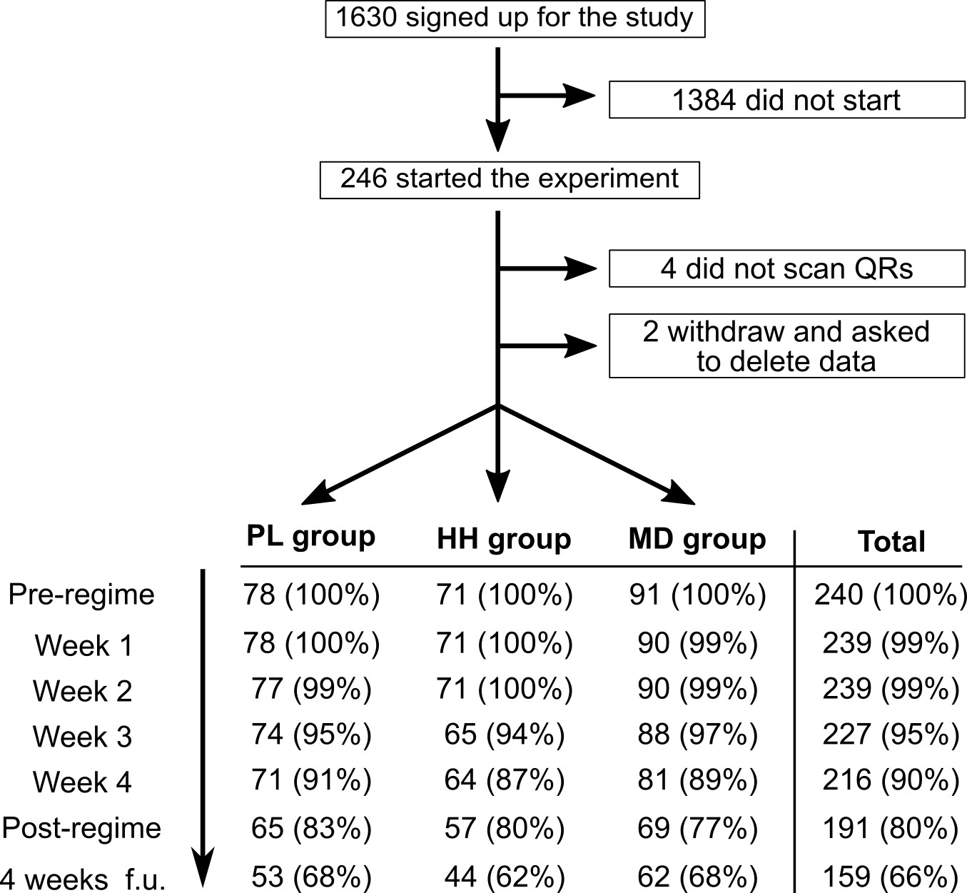
Flow diagram showing participation and completion rates through the study.

The completion of the 4 weeks follow-up timepoint was optional.

Figure 4

Download asset Open asset

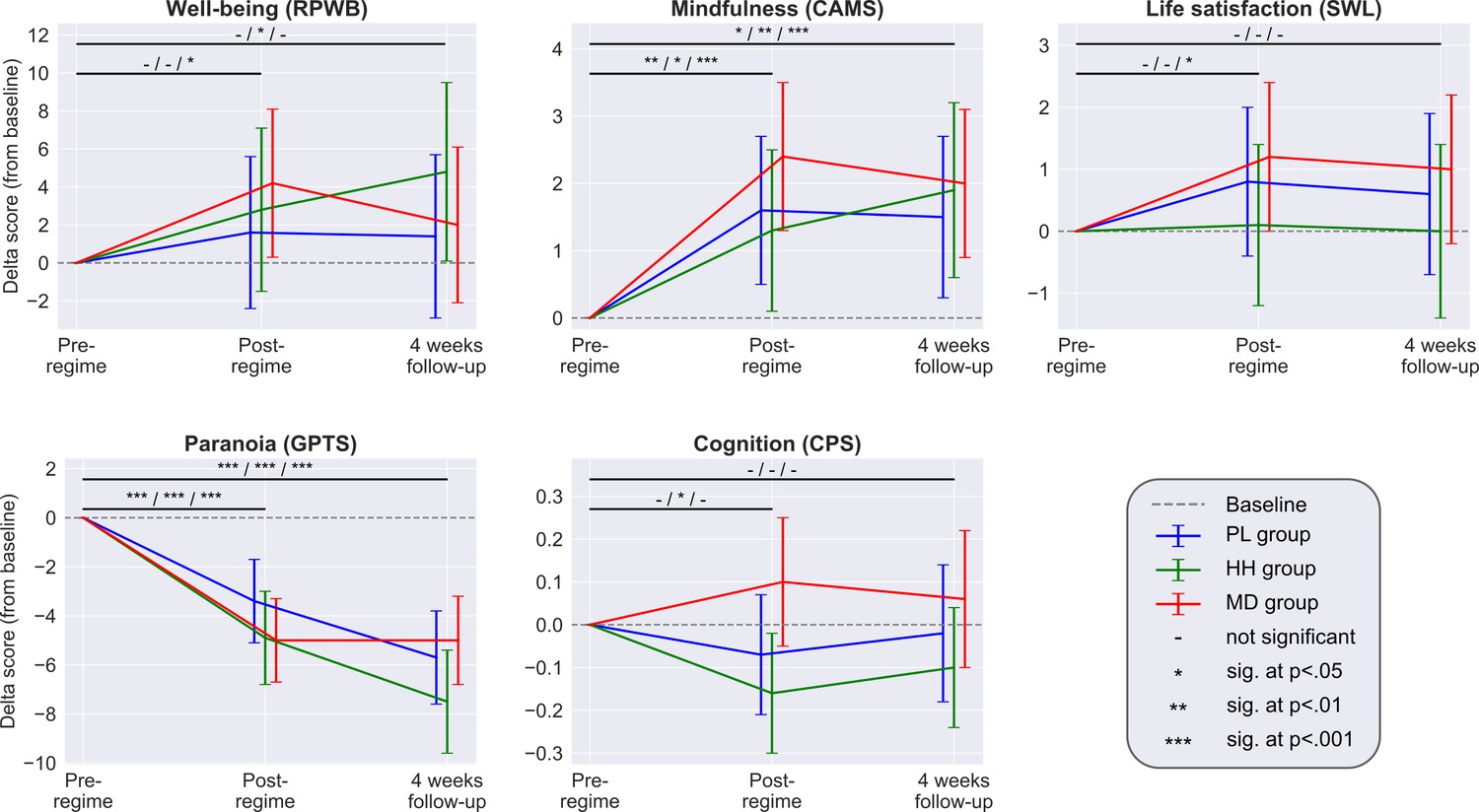
Each panel shows the adjusted mean estimate of the change from baseline and the 95% CI for the accumulative outcomes.

Top horizontal bars represent the over time comparisons for each group (from baseline to post-regime [week 5] and from baseline to follow-up). Symbols on top of bars show the significance for the PL/HH/MD groups, respectively (e.g. change from baseline to post-regime in well-being was significant for the MD group, but not significant for the other two groups, see legend). There was no significant between-groups difference at any timepoint for any scale. Sample size was 240/191/159 at the pre-, post-regime and 4 weeks follow-up timepoints, respectively. See Supplementary files 4, 5, and 6 for the unadjusted descriptive statistics, adjusted mean differences (and their significance) associated with both over time and between group comparisons and model parameters, respectively.

Figure 5

Download asset Open asset

Acute and post-acute outcomes stratified by guess and condition.

On each panel, the four bars represent the adjusted mean estimates and the associated 95% CI of the four strata corresponding to the four combinations of guess (PL/MD) and condition (PL/MD). For the psychological measures (all, but CPS) the sample size was 857 (participants contributed four scores corresponding to the four acute/post-acute assessment timepoints during the dose period), while for cognitive performance it was 684, see bottom of each panel for the condition, guess, and the proportion of scores in the given strata. Top horizontal lines represent comparisons between strata derived from the models. The two short lines on top are the comparisons between PL and MD conditions with fixed guess, while the two longer lines below are the comparisons between PL and MD guesses with fixed drug condition, see Supplementary file 8 for numerical results. Note that for all self-reported outcomes, change in guess is almost always significant, while a change in condition is never significant. In the case of cognitive performance, neither change in guess nor change in condition is significant.

Appendix 1—figure 1

Download asset Open asset

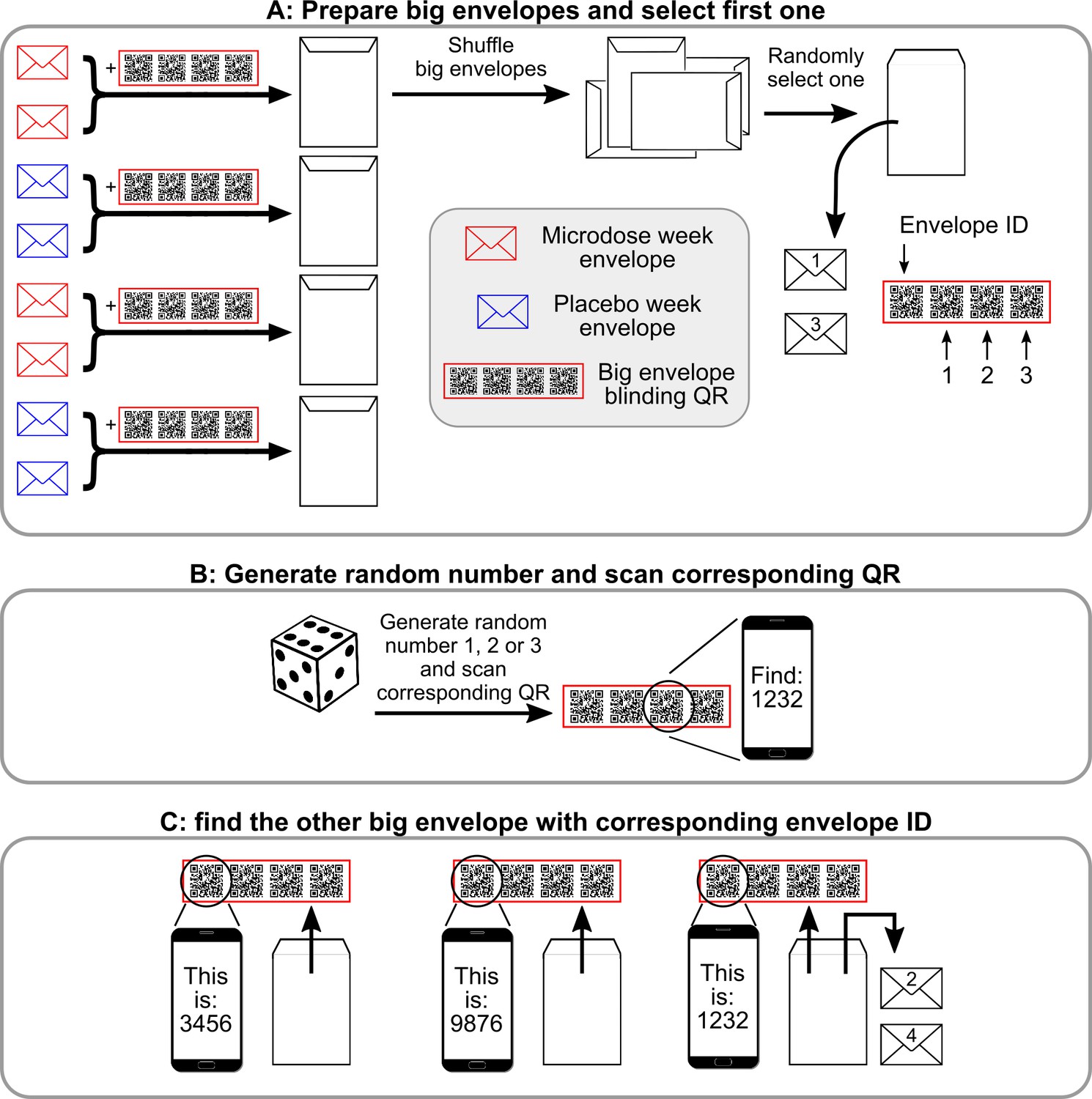
Semi-random drawing process during the self-blinding setup, which corresponds to panel B of Figure 2 in the main text.

After the eight envelopes are prepared, pairs of microdose and placebo envelopes are placed inside big envelopes together with the corresponding ‘big envelope QR’ (a set of four QRS in the red frame) and then sealed. Once each big envelope is assembled, they are shuffled, and one is randomly selected. ‘1’ and ‘3’ are written on the two small envelopes inside (that contain the capsules and the weekly QR code, see Figure 2 of the main text) to designate that these will be used for weeks 1 and 3 (Panel A). Next, the other big envelope needs to be selected with the help of the big envelope QRs. Each big envelope QR has four QR codes: *envelope id* and *1,2,3*. First, a random number is generated between 1 and 3 (dice roll) and the corresponding QR is scanned (Panel B). Scanning displays a message ‘You need to find big envelope with ID XXXX’. Then, a random big envelope is opened and the ‘Envelope ID’ field is scanned from the big envelope QR inside. Scanning displays ‘This big envelope’s ID is YYYY’. This process is continued until big envelope XXXX is found. ‘2’ and ‘4’ are written on the two small envelopes inside to designate that these will be used for weeks 2 and 4.

Appendix 1—figure 2

Download asset Open asset

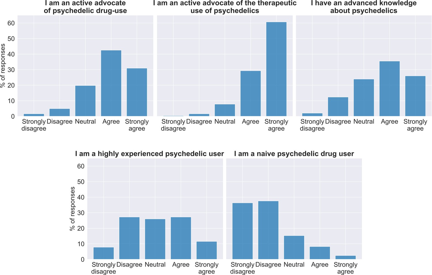
Attitude toward psychedelics in the sample at baseline.

At the top of each panel is the item answered and below the bar graphs show the percentage of participant responses (n = 240).

Appendix 1—figure 3

Download asset Open asset

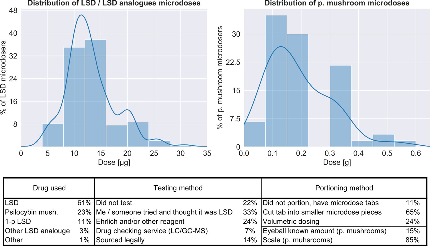
Characteristics of the microdoses used by participants.

Top panel shows the distribution of doses for both LSD/LSD analogues (n = 180, 12.8 ± 5.5 μg) and psilocybin containing mushrooms (n = 56, 0.19 ± 0.12 g), bottom table provides additional information on the microdose preparation.

Tables

Table 1

List of outcomes.

Outcomes have three types, depending on what is the timescale of the effect they aim to capture: accumulative are monthly, post-acute are the weekly and acute are the daily effects. A scale is administered at every timepoint of the associated outcome type if the checkmark is shown, for example, PANAS was administered at every acute timepoint, that is every Thursday during the dose period, see Figure 1 for a visual overview of the timepoints and see Appendix 1 for a description of each scale.

Test	Domain	Acronym	Baseline	Acute	Post-acute	Accumulative
Demographics	-	-	✔
Previous drug experiences and expectations	-	-	✔
Short suggestibility scale	Suggestibility	SSS	✔
Cognitive performance score	Cognition	CPS	✔	✔		✔
Daily effects of microdosing VASs	-	-		✔
Positive and negative affection scale	Emotional state	PANAS		✔
Warwick–Edinburgh mental well-being scale	Well-being	WEMWB			✔
Quick inventory of depressive symptomatology	Depression	QIDS			✔
Social connectedness scale	Connectedness	SCS			✔
Spielberger’s state-trait anxiety inventory	Anxiety	STAIT			✔
Ryff’s psychological well-being scales	Well-being	RPWB	✔			✔
Cognitive and affective mindfulness scale	Mindfulness	CAMS	✔			✔
Green paranoid thought scales	Paranoia	GPTS	✔			✔
Big five personality inventory	Personality	B5	✔			✔
Satisfaction with life	Life satisfaction	SWL	✔			✔

Table 2

Summary of acute and post-acute outcomes.

Acute outcomes were measured on dosing days (Thursdays), while the potential microdose was still active, comparison is made between scores obtained under the influence of microdose vs placebo capsules. Post-acute outcomes were measured at the end of the weeks (Sundays), when no capsule was taken, and comparison is made between scores obtained at the end of placebo weeks vs microdose weeks. For the psychological measures (all except CPS) the sample size was 857 (participants contributed four scores corresponding to the four acute/post-acute assessment timepoints during the dose period), while for cognitive performance it was 684. The first three columns show the unadjusted, observed scores and Cohen’s d between the two conditions (PL/MD). In the next column, results from the models without the guess component are shown, and last column shows model results with the guess component, each cell shows the adjusted mean difference ±95% CI of condition (PL vs. MD, where PL is used as baseline), see Materials and methods for details. Individual subscales/sub-tasks are shown when they exist (in the Test column, ‘X – y’ denotes that y is a subscale or sub-test of X).

	Observed scores			Model wo. guess	Model with guess
Test	PL (M ± 95% CI)	MD (M ± 95% CI)	Cohen's d	M ± 95% CI	M ± 95% CI
Acute outcomes
Acute mood (PANAS)	14.2 ± 0.9	16.2 ± 1.1	0.19	2.2 ± 1.4**	0.9 ± 1.4
PANAS – positive	29.9 ± 0.7	31.6 ± 0.8	0.22	2.0 ± 1.0***	0.8 ± 1.0
PANAS – negative	15.7 ± 0.5	15.4 ± 0.5	−0.06	−0.4 ± 0.7	−0.3 ± 0.8
Daily effects VAS – intensity	8.5 ± 1.6	21.4 ± 2.7	0.58	12.5 ± 3.0***	3.4 ± 2.0***
Daily effects VAS – energy	55.3 ± 1.8	60.7 ± 2.1	0.27	5.3 ± 2.7***	2.4 ± 2.8
Daily effects VAS – mood	60.5 ± 1.8	64.7 ± 2.2	0.20	4.6 ± 2.9***	1.5 ± 2.8
Daily effects VAS – creativity	53.5 ± 1.6	58.3 ± 2.0	0.25	4.7 ± 2.6***	1.8 ± 2.6
Daily effects VAS – focus	57.3 ± 1.7	58.7 ± 2.1	0.07	1.3 ± 2.8	−0.6 ± 2.8
Daily effects VAS – temper	36.5 ± 2.0	36.0 ± 2.5	−0.02	−1.3 ± 3.2	0.1 ± 3.2
Cognition (CPS)	−0.08 ± 0.05	−0.06 ± 0.07	0.05	0.05 ± 0.08	0.04 ± 0.07
CPS – rotations	−0.09 ± 0.09	−0.06 ± 0.11	0.03	0.11 ± 0.14	0.12 ± 0.14
CPS – odd one out	0.02 ± 0.11	0.14 ± 0.1	0.12	0.09 ± 0.16	0.08 ± 0.16
CPS – spatial planning	−0.11 ± 0.1	−0.1 ± 0.11	0.00	0.04 ± 0.14	0.03 ± 0.14
CPS – spatial span	−0.18 ± 0.09	−0.18 ± 0.11	0.00	0.01 ± 0.14	0.02 ± 0.14
CPS – feature match	−0.06 ± 0.09	−0.05 ± 0.13	0.00	−0.05 ± 0.15	−0.07 ± 0.16
CPS – paired associates	−0.1 ± 0.09	−0.11 ± 0.12	−0.02	0.05 ± 0.15	0.05 ± 0.15
Post-acute outcomes
Mental well-being (WEMWB)	49.7 ± 0.8	49.8 ± 0.7	0.02	0.9 ± 1.0	0.1 ± 1.0
Depression (QIDS)	5.6 ± 0.5	5.5 ± 0.4	−0.03	−0.3 ± 0.6	−0.1 ± 0.6
Anxiety trait (STAI-T)	38.5 ± 1.2	38.1 ± 1.0	−0.04	−1.5 ± 1.3*	−0.1 ± 0.6
Social conn. (SCS)	32.1 ± 0.7	32.1 ± 0.6	0.00	0.1 ± 0.8	−0.3 ± 0.8

*=p<0.05; **=p<0.01; ***=p<0.001.

Appendix 1—table 1

Comparison of guessing performance to a random guesser.

X/Y (in the header columns) denotes condition X and guess Y. Sensitivity is the ratio of true positives to all positives (i.e. MD guessed and taken/MD taken), specificity is the ratio of true negatives to all negatives (i.e. PL guessed and taken/PL taken), while F1 is the harmonic mean of these metrics, used as a single number summary of accuracy. Sensitivity is not defined for the PL group, as they never take a microdose.

	True positive rate (MD/MD)	False negative rate (MD/PL)	False positive rate (PL/MD)	True negative rate (PL/PL)	Sensitivity	Specificity	F1-score
PL group participants	0	0	0.21	0.79	-	0.79	0
HH group participants	0.14	0.12	0.12	0.62	0.54	0.84	0.54
MD group participants	0.21	0.3	0.08	0.41	0.41	0.84	0.53
All participants	0.12	0.15	0.13	0.59	0.45	0.82	0.46
Random guesser	0.06	0.19	0.19	0.56	0.25	0.75	0.25