Figures and data in Estimation and worldwide monitoring of the effective reproductive number of SARS-CoV-2

Figures
Tables
Additional files

24 figures, 6 tables and 3 additional files

Figures

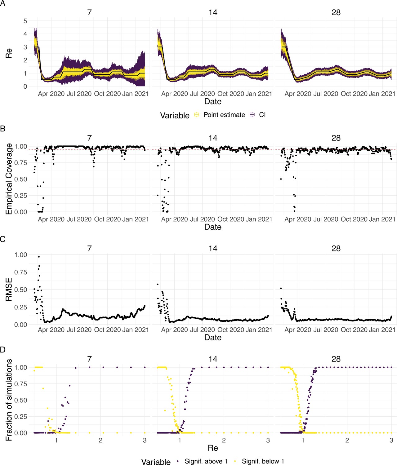
Figure 1

Download asset Open asset

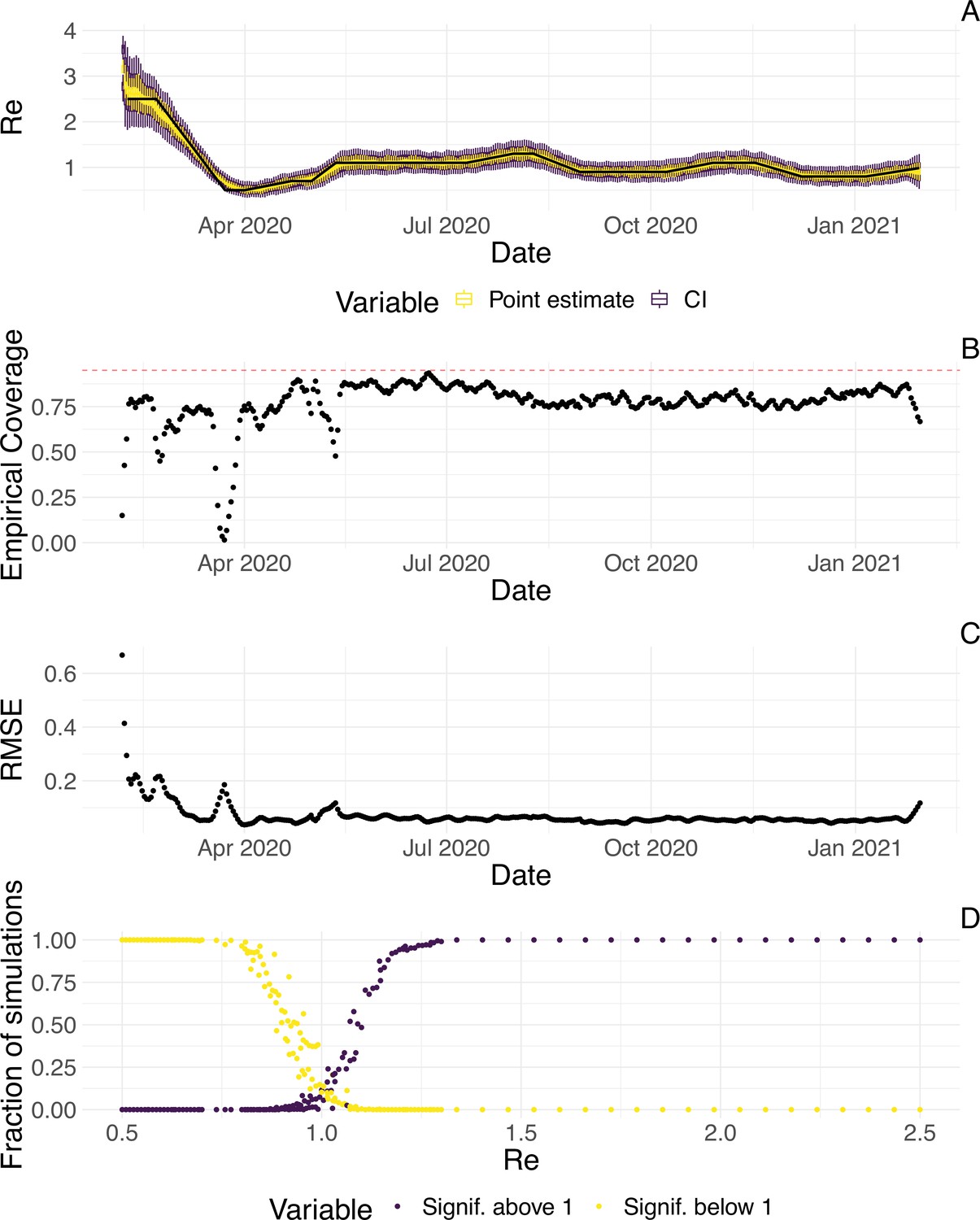
Evaluation of the pipeline on simulated data.

(A) The specified $R_{e}$ trajectory (black line) was used to stochastically simulate 100 trajectories of observed cases. From each trajectory, we estimated $R_{e}$ (yellow boxplots) and constructed a 95% confidence interval (purple boxplots of the lower/upper endpoint). (B) Fraction of simulations for which the true $R_{e}$ value was within the 95% confidence interval. The dashed red line indicates the nominal 95% coverage. (C) Root mean squared relative error for every time point. (D) Fraction of simulations for which $R_{e}$ is estimated to be significantly above or below one, depending on the true value of $R_{e}$ .

Figure 2

Download asset Open asset

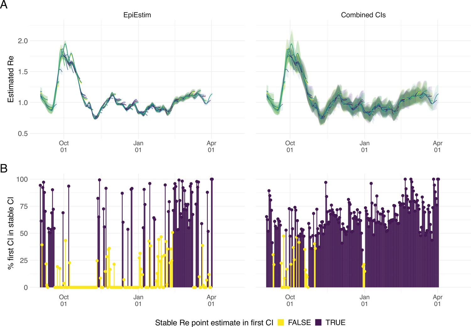
Stability of the Swiss $R_{e}$ estimates based on confirmed COVID-19 cases, upon adding additional days of observations.

(A) Line segments correspond to 3 weeks of estimates made with the same input data (e.g. data up to December 1st). The segments were assigned an arbitrary colour for ease of distinction. For each day, $R_{e}$ estimates and associated 95% confidence intervals (CIs) are overlaid, from the first possible estimate for that day up to estimates including 3 additional weeks of data. The latter, always the left end of a line segment, corresponds to the stable estimate. (B) Percentage of the first estimated CI that is contained in the stable CI based on data from 30 April 2021. This percentage was calculated as the width of the intersection of both CIs, divided by the width of the first CI. The colour indicates whether the stable $R_{e}$ estimate was contained in the first reported CI. In both rows, the left column shows uncertainty intervals from EpiEstim on the original data, and the right our improved 95% CIs. Both columns use the same pipeline, and differ only in the construction of the uncertainty intervals.

Figure 3

Download asset Open asset

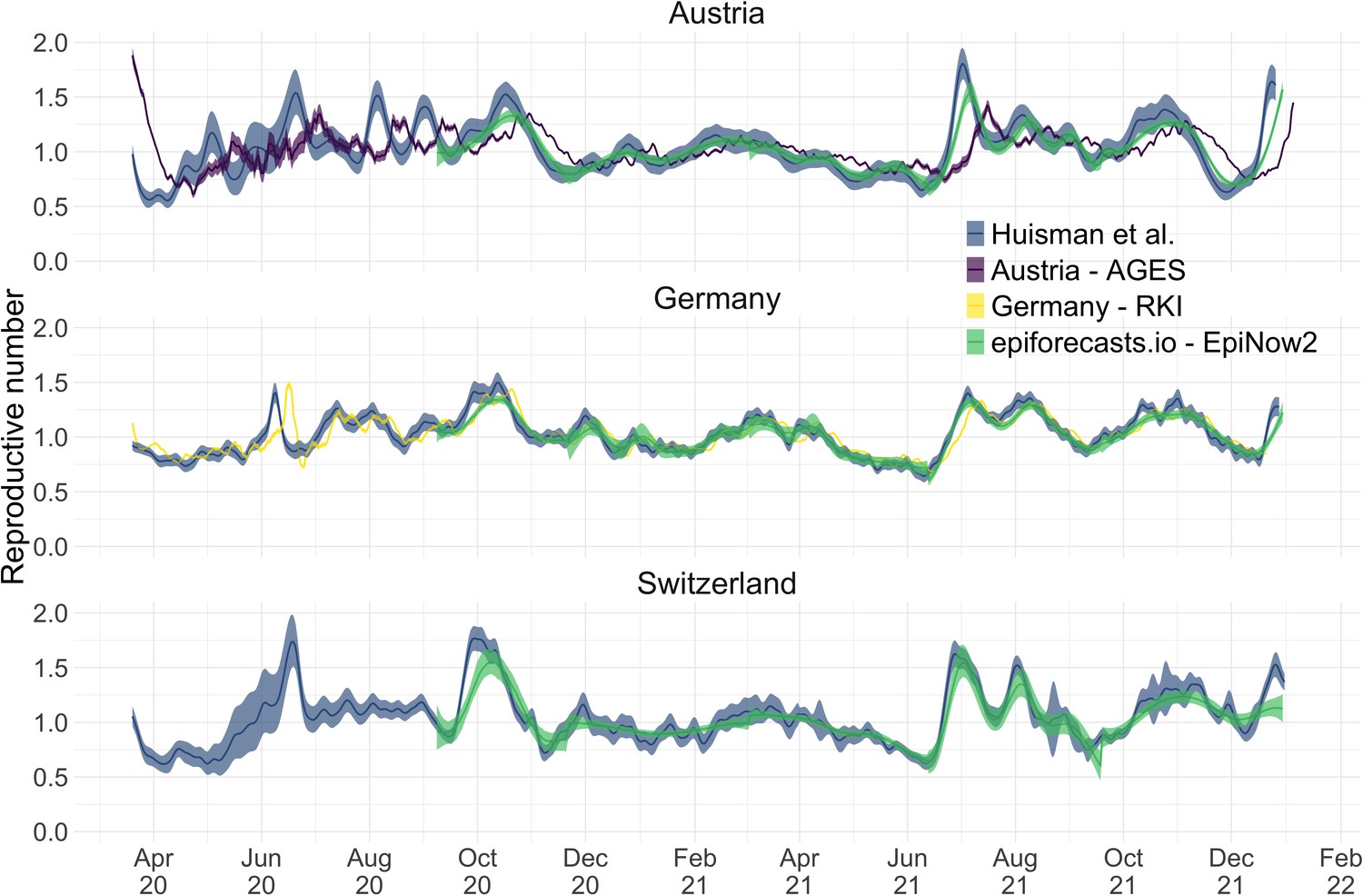
Comparison of published $R_{e}$ estimates for three countries.

Point estimates are presented with a solid line and 95% confidence intervals are presented as coloured ribbons.

Figure 4

Download asset Open asset

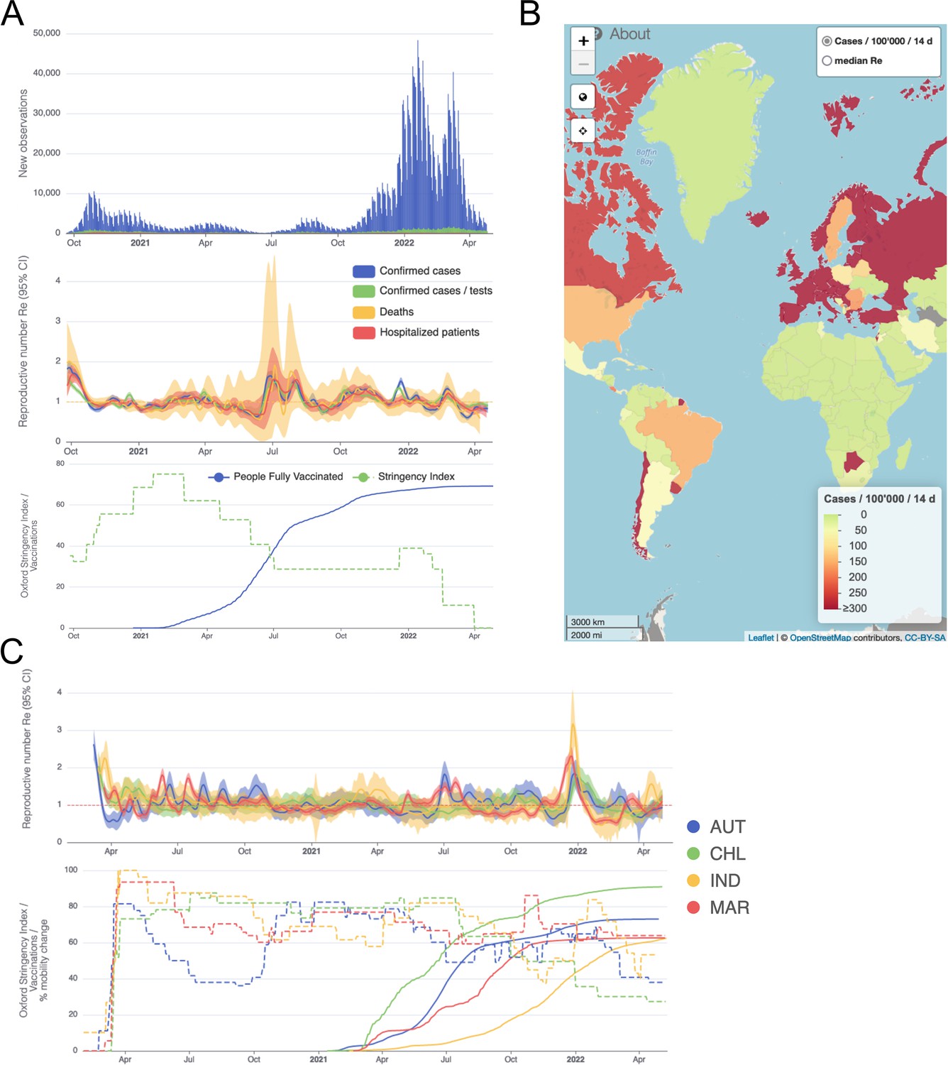
Example panels from the online dashboard.

(A) Swiss case incidence with evidence of weekly testing patterns (top row), $R_{e}$ estimates with associated 95% confidence intervals from four types of observation data (middle row), and timeline of stringency index and vaccination coverage (bottom row). (B) World map of incidence per 100’000 inhabitants over the last 14 days. One can also display the worldwide $R_{e}$ estimates instead. (C) Comparison of $R_{e}$ estimates across four countries (Austria, Chile, India and Morocco), with timelines of stringency indices and vaccination coverage. All panels were extracted on May 12, 2022. Dashboard url: https://ibz-shiny.ethz.ch/covid-19-re-international.

Figure 5

Download asset Open asset

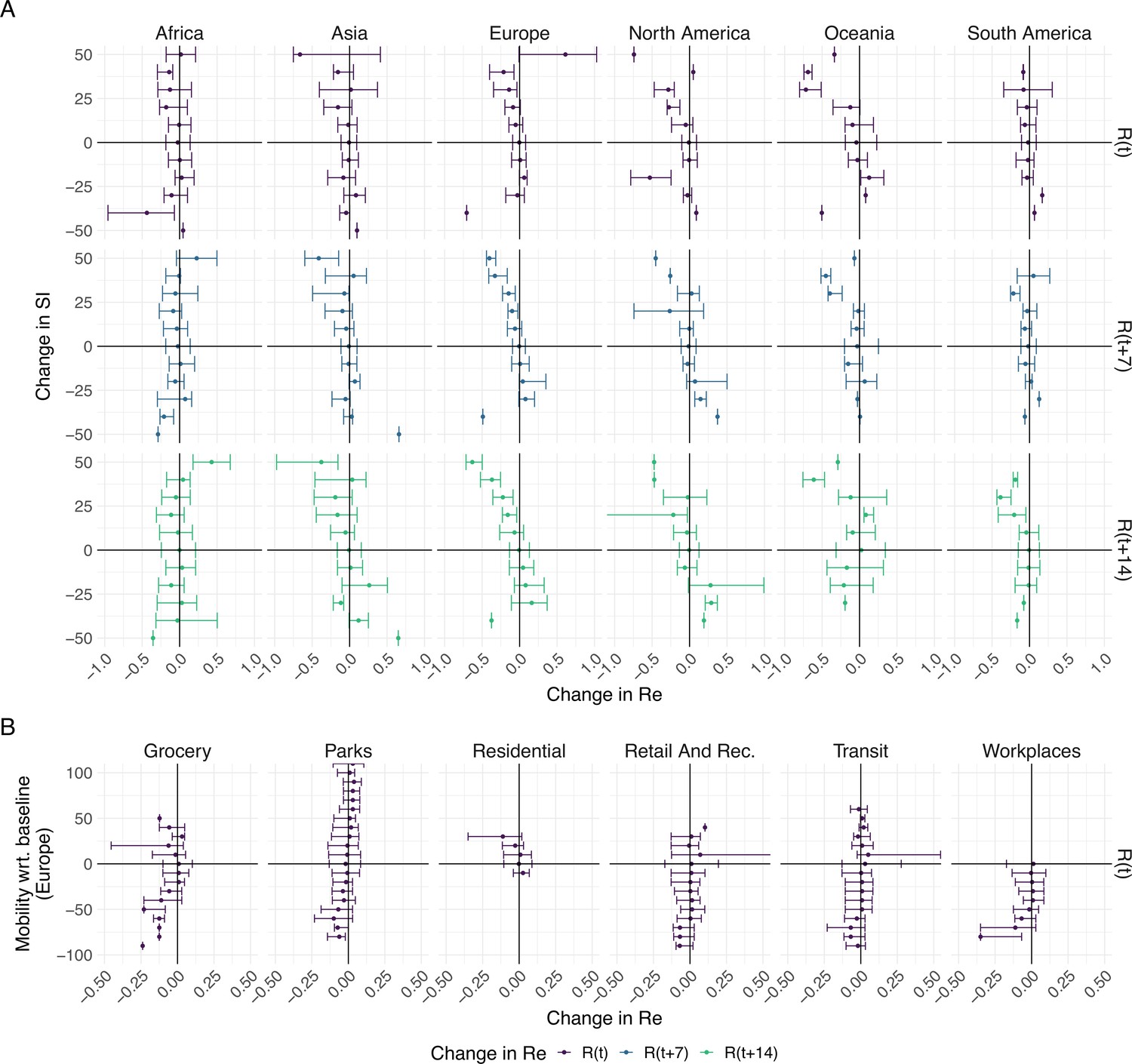
The association between the implementation or lifting of non-pharmaceutical interventions and changes in $R_{e}$ until May 2021.

(A) The change in the estimated $R_{e}$ at the same time as ( $R (t)$ ) or following ( $R (t + 7)$ and $R (t + 14)$ ) the implementation (above x-axis) or lifting (below x-axis) of NPIs in a given week. (B) The change in the estimated $R_{e}$ related to the change in mobility in the same week. The error bars indicate the Q1 and Q3 quartiles.

Appendix 2—figure 1

Download asset Open asset

Schematic of the effect of smoothing on the ability to estimate when $R_{e} = 1$ .

The true $R_{e}$ is indicated by the black solid line, the black dashed line shows a linear approximation of the smoothed $R_{e}$ . Instead of crossing 1 at $t_{0}$ , this line crosses 1 at $t_{0} + s$ .

Appendix 3—figure 1

Download asset Open asset

Performance of our method on simulated scenarios with differing slopes.

(A) The specified $R_{e}$ trajectory (black line; see Methods) was used to simulate a trajectory of reported cases (with Swiss case observation noise) 100 times. From each trajectory we estimated $R_{e}$ (yellow boxplots), and constructed a 95% confidence interval (purple boxplots of the lower/upper endpoint). We varied the time it took to change from one $R_{e}$ value to the next, $t \in {7, 14, 28}$ (columns). Larger values of $t$ correspond to less abrupt changes. (B) The fraction of simulations where the true $R_{e}$ value was within the 95% confidence interval. The dashed red line indicates the nominal 95% coverage. (C) The root mean squared relative error for every time point. (D) The fraction of simulations where we estimate $R_{e}$ is significantly above or below one, depending on the true value of $R_{e}$ . We see that the method closely tracks the true $R_{e}$ in all scenarios, although the error is greater for steeper slopes. In the case of steeper changes in $R_{e}$ the overall size of the epidemic is also smaller, which explains the larger confidence intervals.

Appendix 3—figure 2

Download asset Open asset

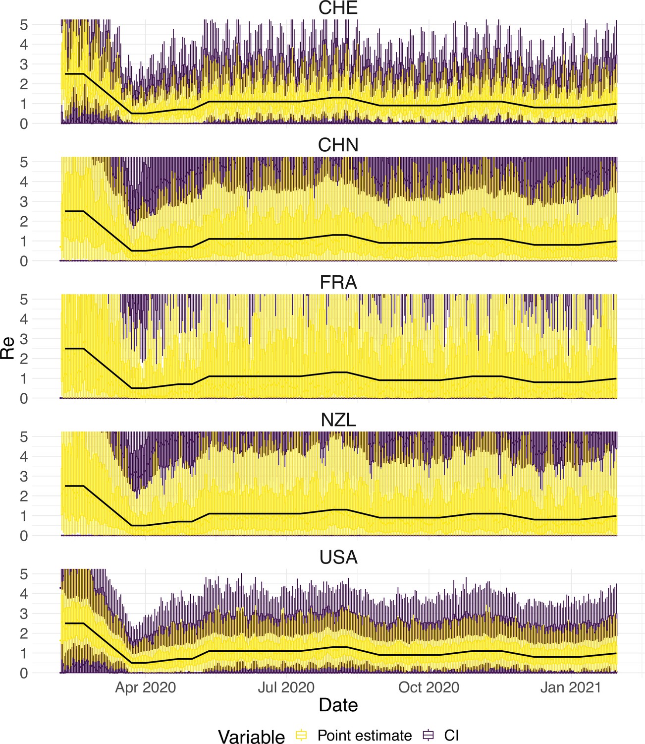
Performance of our method, modified to skip the smoothing step in the pipeline, on simulated scenarios with observation noise.

The specified $R_{e}$ trajectory (black line; see Methods) was used to simulate a trajectory of reported cases (with varying country-specific noise profiles; rows) 100 times. From each trajectory we estimated $R_{e}$ (yellow boxplots), and constructed a 95% confidence interval (purple boxplots of the lower/upper endpoint). Contrary to our normal pipeline, the observations were not smoothed prior to the deconvolution and $R_{e}$ estimation. We see that the estimates are highly variable.

Appendix 3—figure 3

Download asset Open asset

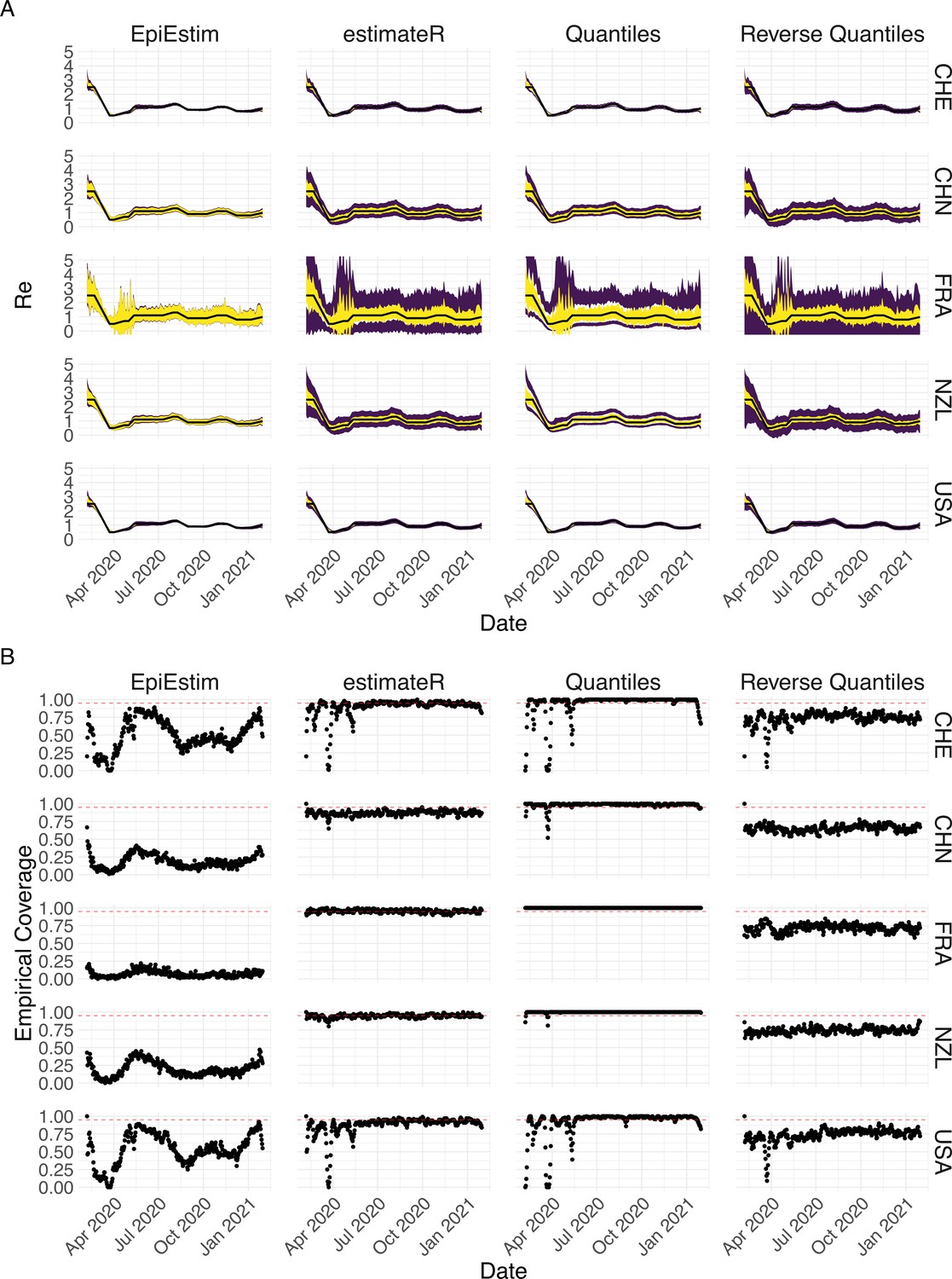
Performance of our method on simulated scenarios with observation noise.

The columns differ in the method used to construct confidence intervals: EpiEstim reports the 95% HPD of EpiEstim on the original data, estimateR refers to our method, Quantiles and Reverse Quantiles use the 5 and 95% quantiles of the estimated $R_{e}$ to construct the CIs. (A) The specified $R_{e}$ trajectory (black line; see Methods) was used to simulate a trajectory of reported cases (with varying country-specific noise profiles; rows) 100 times. From each trajectory we estimated $R_{e}$ (yellow ribbons represent the estimated mean ± sd across 100 simulations), and constructed a 95% confidence interval (purple ribbons represent the mean ± sd of the estimated lower/upper endpoint). (B) The fraction of simulations where the true $R_{e}$ value was within the 95% confidence interval. The dashed red line indicates the nominal 95% coverage.

Appendix 3—figure 4

Download asset Open asset

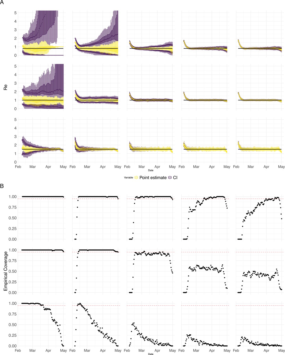
Performance of our method on simulated scenarios with varying population size, using confidence intervals from EpiEstim.

(A) We specified a constant $R_{e} \in {0.8, 1, 1.5}$ value (black line; rows) to simulate a trajectory of reported cases (with Swiss case observation noise) 100 times. From each trajectory we estimated $R_{e}$ (yellow boxplots), and constructed a 95% confidence interval (purple boxplots of the lower/upper endpoint). The simulated scenarios had differing initial incidence of $I_{0} \in {10, 100, 1000, 5000, 10000}$ infections per day (columns). In the top row, $R_{e} < 1$ so the epidemic is decreasing. In the middle row, $R_{e} = 1$ , the epidemic is constant, and in the bottom row, $R_{e} > 1$ , the epidemic is increasing. The bias at the start is due to the initialisation of the simulation. (B) The fraction of simulations where the true $R_{e}$ value was within the 95% confidence interval. The dashed red line indicates the nominal 95% coverage. We see that the EpiEstim coverage strongly declines with increased epidemic size.

Appendix 3—figure 5

Download asset Open asset

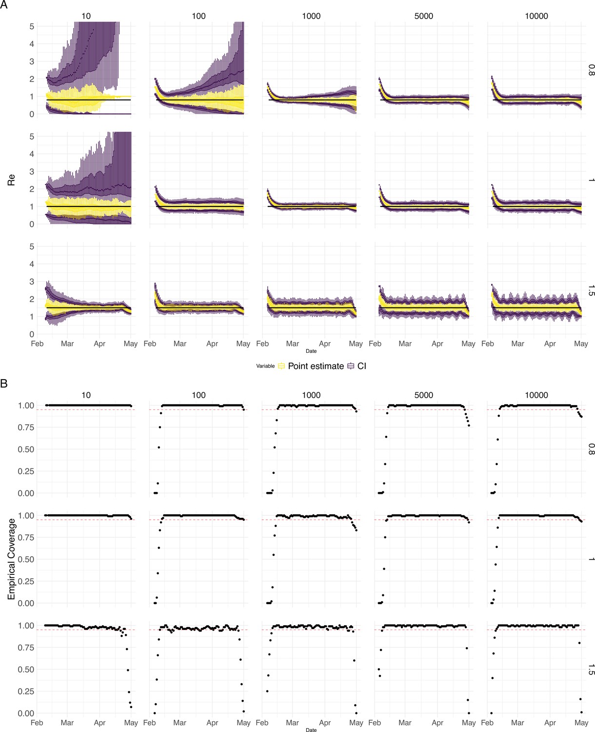
Performance of our method on simulated scenarios with varying population size, using the Union of EpiEstim and Block bootstrap 95% confidence intervals.

(A) We specified a constant $R_{e} \in {0.8, 1, 1.5}$ value (black line; rows) to simulate a trajectory of reported cases (with Swiss case observation noise) 100 times. From each trajectory we estimated $R_{e}$ (yellow boxplots), and constructed a 95% confidence interval (purple boxplots of the lower/upper endpoint). The simulated scenarios had differing initial incidence of $I_{0} \in {10, 100, 1000, 5000, 10000}$ infections per day (columns). In the top row, $R_{e} < 1$ so the epidemic is decreasing. In the middle row, $R_{e} = 1$ , the epidemic is constant, and in the bottom row, $R_{e} > 1$ , the epidemic is increasing. The bias at the start is due to the initialisation of the simulation. (B) The fraction of simulations where the true $R_{e}$ value was within the 95% confidence interval. The dashed red line indicates the nominal 95% coverage. We see that for a wide range of infection incidences, our 95% confidence interval is informative and covers the true value of $R_{e}$ .

Appendix 3—figure 6

Download asset Open asset

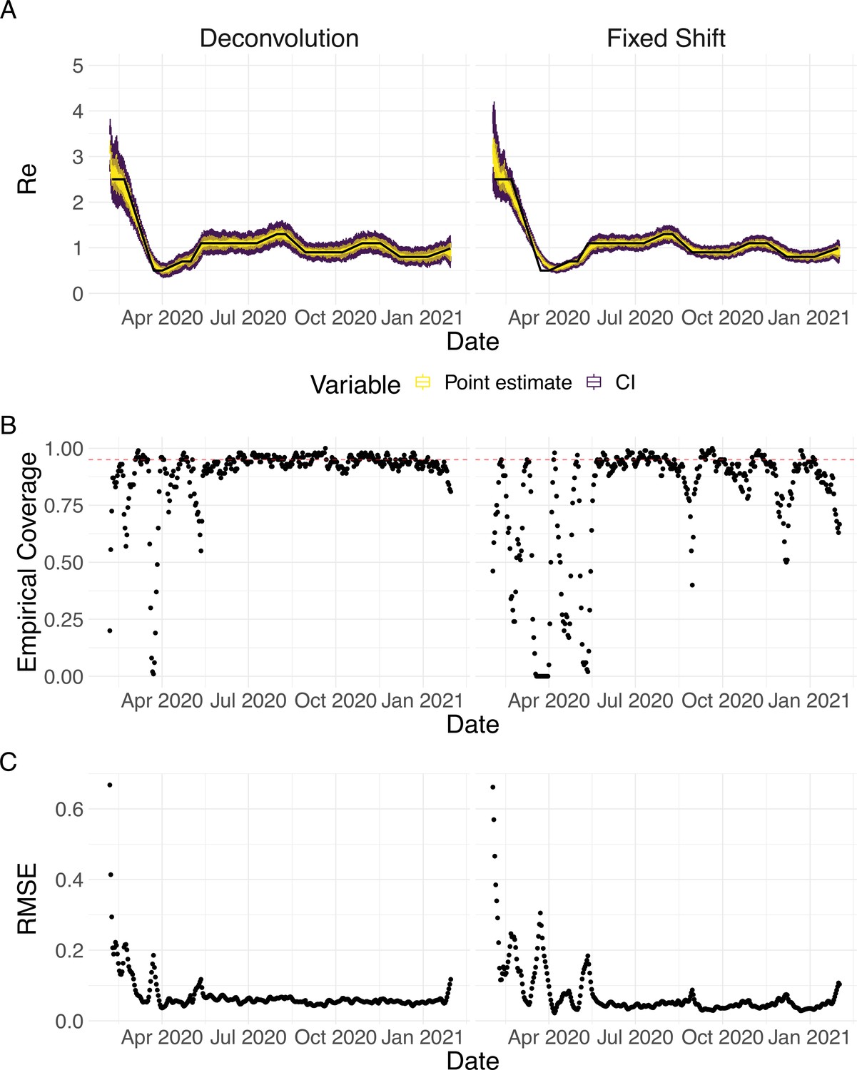
Performance of our method on simulated scenarios using a fixed shift versus the deconvolution to infer infection incidence.

The fixed shift method shifts the observations back by the mean of the delay distribution (here assumed to correspond to confirmed cases). (A) The specified $R_{e}$ trajectory (black line; see Methods) was used to simulate a trajectory of reported cases (with Swiss case observation noise) 100 times. From each trajectory we estimated $R_{e}$ (yellow boxplots), and constructed a 95% confidence interval (purple boxplots of the lower/upper endpoint). (B) The fraction of simulations where the true $R_{e}$ value was within the 95% confidence interval. The dashed red line indicates the nominal 95% coverage. The average coverage in this scenario was 0.90 with deconvolution and 0.78 with the fixed shift. (C) The root mean squared relative error for every time point. The average (cumulative) RMSE in this scenario was 0.0706 (25.4) with deconvolution and 0.0726 (26.6) with the fixed shift.

Appendix 3—figure 7

Download asset Open asset

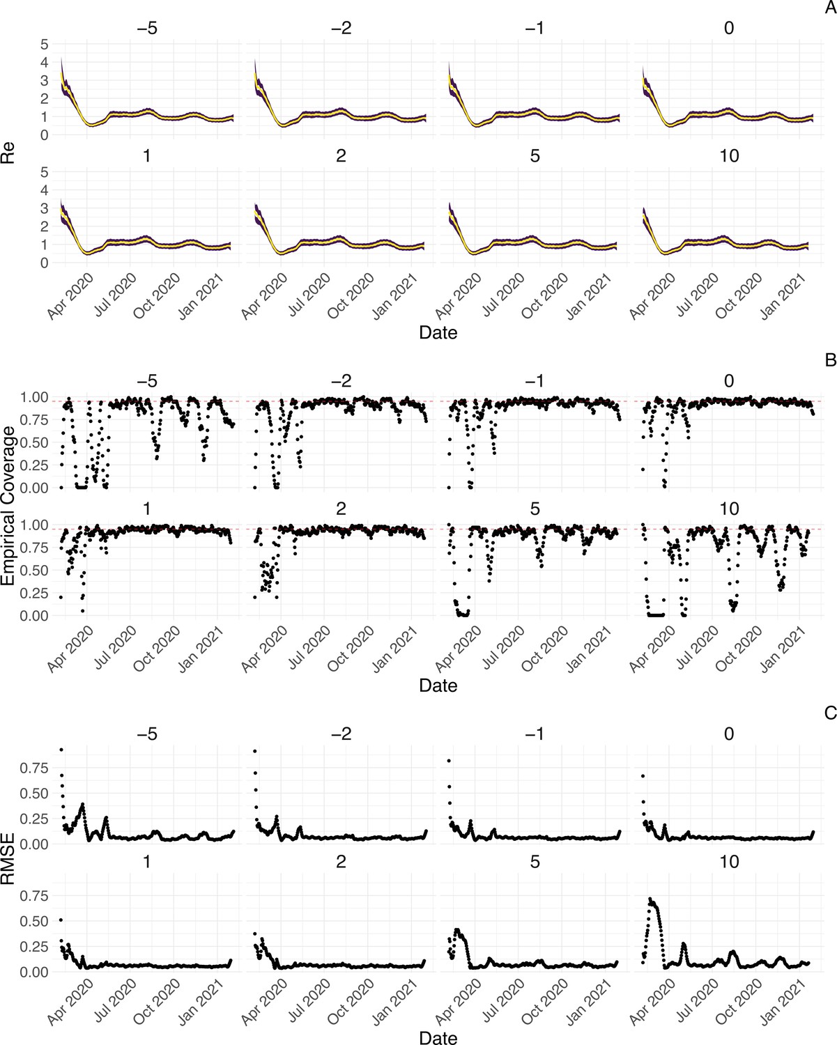
Performance of our method on simulated scenarios with misspecified delay distributions.

When estimating $R_{e}$ , we misspecified the mean of the delay distribution (5.5 for symptom-onset to case confirmation) by the numbers above the columns. (A) The specified $R_{e}$ trajectory (black line; see Methods) was used to simulate a trajectory of reported cases (with Swiss case observation noise) 100 times. From each trajectory we estimated $R_{e}$ (yellow boxplots), and a 95% confidence interval (purple boxplots of the lower/upper endpoint). (B) The fraction of simulations where the true $R_{e}$ value was within the 95% confidence interval. The dashed red line indicates the nominal 95% coverage. The average coverage in this scenario was 0.72, 0.85, 0.88, 0.90, 0.90, 0.89, 0.82, 0.69 from –5 to 10. (C) The root mean squared relative error for every time point. The average (cumulative) RMSE in this scenario was 0.0989 (36.0), 0.0807 (29.2), 0.0746 (26.9), 0.0706 (25.4), 0.0701 (25.2), 0.0726 (26.0), 0.0909 (32.3), 0.134 (47.0) from –5 to 10.

Appendix 3—figure 8

Download asset Open asset

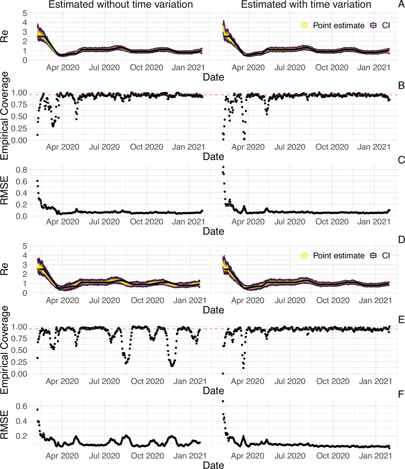
Performance of our method on simulated scenarios with time-varying delay distributions.

The observations were simulated with a time-varying delay distribution for (**A,B,C**) confirmed cases, or (**D,E,F**) deaths (see Methods), and then estimated with (right column) or without (left column) taking the time-varying distributions into account. (**A, D**) The specified $R_{e}$ trajectory (black line; see Methods) was used to simulate a trajectory of reported cases or deaths (with Swiss case observation noise) 100 times. From each trajectory we estimated $R_{e}$ (yellow boxplots), and a 95% confidence interval (purple boxplots of the lower/upper endpoint). (**B, E**) The fraction of simulations where the true $R_{e}$ value was within the 95% confidence interval. The dashed red line indicates the nominal 95% coverage. For the cumulative cases, the average coverage in this scenario was 0.89 without and 0.89 with time variation. For the deaths, the average coverage was 0.83 without and 0.92 with time variation. (**C, F**) The root mean squared relative error for every time point. For the cumulative cases, the average (cumulative) RMSE was 0.0728 (26.2) without and 0.0783 (28.5) with time variation. For the deaths, the average (cumulative) RMSE was 0.113 (39.5) without and 0.0861 (30.8) with time variation.

Appendix 4—figure 1

Download asset Open asset

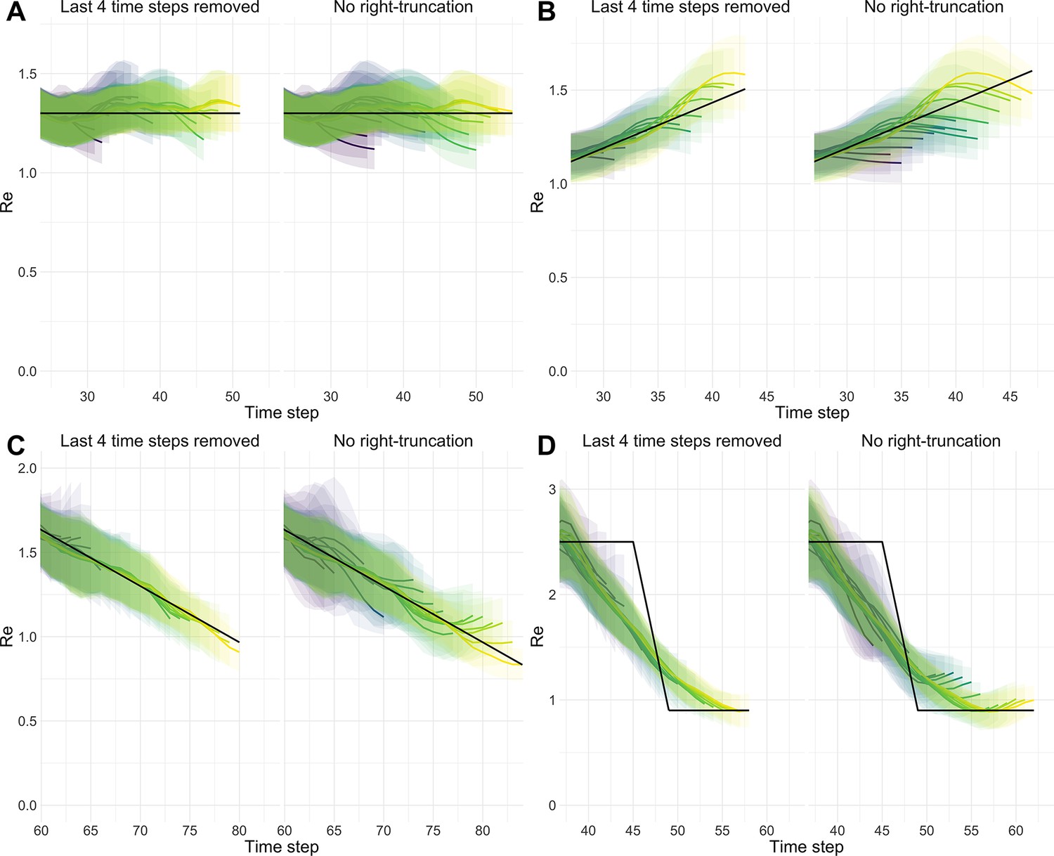
Stability of $R_{e}$ estimates at present.

We estimated $R_{e}$ through time repeatedly on 4 scenarios. With each new iteration, we added one new data point at present. Each $R_{e}$ trajectory is presented with its own colour. Purple trajectories are iterations for which the last known case data point was furthest in the past, yellow trajectories are trajectories for which the last known case data point was closest to the present. In each panel and for each $R_{e}$ trajectory, 100 simulation replicates were aggregated. The median of mean estimates are presented with lines and medians of upper and lower bounds of 95% confidence intervals are shown with translucent ribbons. For each scenario, two panels are presented. Each time the right panel correspond to raw estimates and the left panel corresponds to the same estimates with the last 4 $R_{e}$ values removed from each $R_{e}$ trajectory. (A) Stable $R_{e}$ . (B) Gradual increase in $R_{e}$ . (C) Gradual decrease in $R_{e}$ . (D) Abrupt decrease in $R_{e}$ .

Appendix 4—figure 2

Download asset Open asset

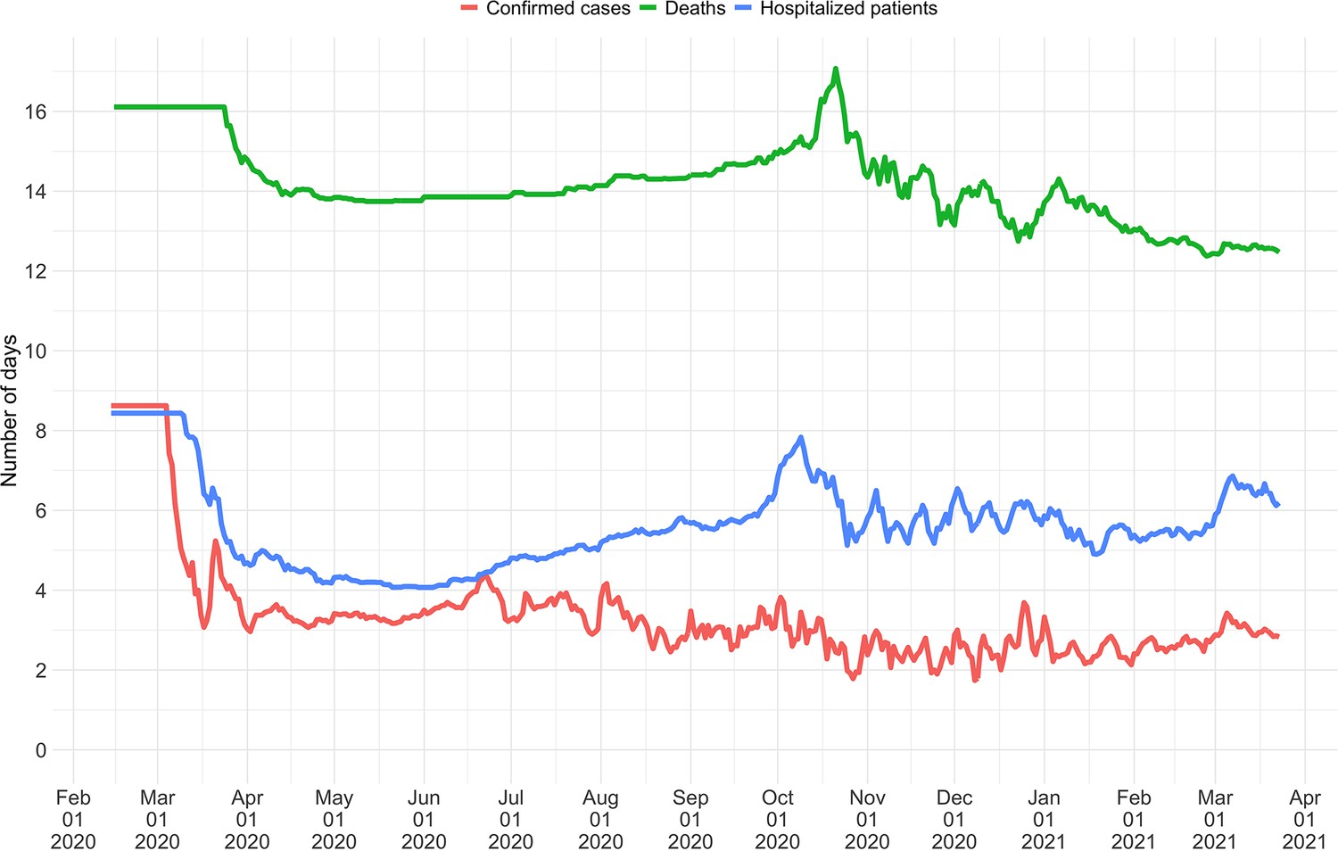
Mean delay in Switzerland between onset of symptoms and reporting.

For each date, the mean is taken over the last 300 reports with known symptom onset date, based on line list data from the FOPH. For early dates, before 300 reports are available, the mean is taken over the first 300 reports.

Appendix 4—figure 3

Download asset Open asset

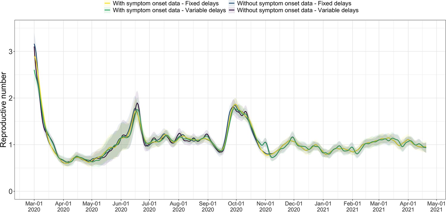
Comparison of the $R_{e}$ estimates with or without accounting for known symptom onset dates and for time-variability on reporting delays.

The comparison is based on time series of confirmed cases in Switzerland, from line list data provided by the FOPH. Both the inclusion of known symptom onset dates and of the time-variability of reporting delay distributions have an effect on the Re estimates, in particular for early estimates in this case. The fraction of cases with known symptom onset date has drastically reduced since November 2020, hence the overlap in curves with and without symptom onset data for later dates. For each trajectory the point estimate is shown with a line, and the translucent ribbon indicates the 95% confidence interval.

Appendix 4—figure 4

Download asset Open asset

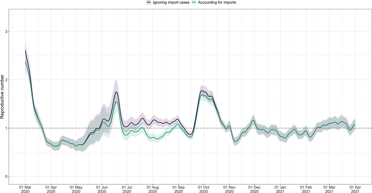
Effective reproductive number estimates with or without accounting for known imports.

The comparison is based on time series of confirmed cases in Switzerland, from line list data provided by the FOPH. The analysis ignoring imports is unbiased if the number of imports equals the number of exports. Since the analysis accounting for imports is not accounting for exports, the results are a lower limit for the effective reproductive number. Very few imported cases were reported since November 2020, hence the complete overlap in the curves after that date. For each trajectory the point estimate is shown with a line, and the translucent ribbon indicates the 95% confidence interval.

Appendix 5—figure 1

Download asset Open asset

Square root and log transformations to stabilise the variance of residuals.

Each row corresponds to the results of observations from Switzerland (CHE), China (CHN), France (FRA), New Zealand (NZL) and the United States (USA), respectively. The first and last two plots correspond to the result of square root transformation and log transformation, respectively.

Appendix 5—figure 2

Download asset Open asset

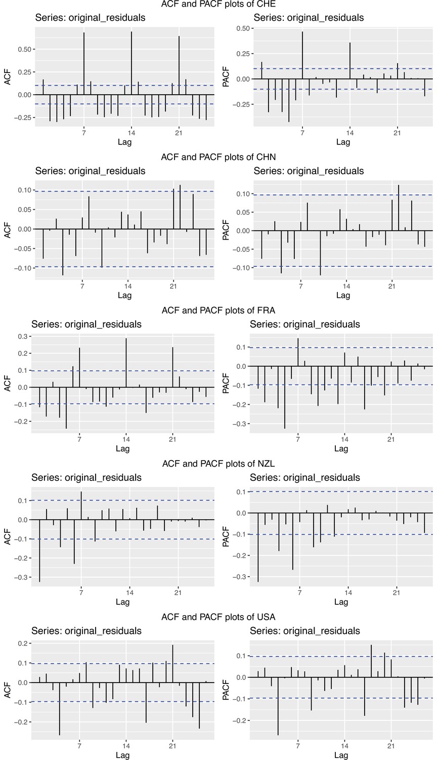
Autocorrelation function (ACF) and partial autocorrelation function (PACF) plots of the observations from five different countries.

In each row, the two plots are the ACF and PACF plots of the observations from Switzerland (CHE), China (CHN), France (FRA), New Zealand (NZL) and the United States (USA), respectively.

Appendix 5—figure 3

Download asset Open asset

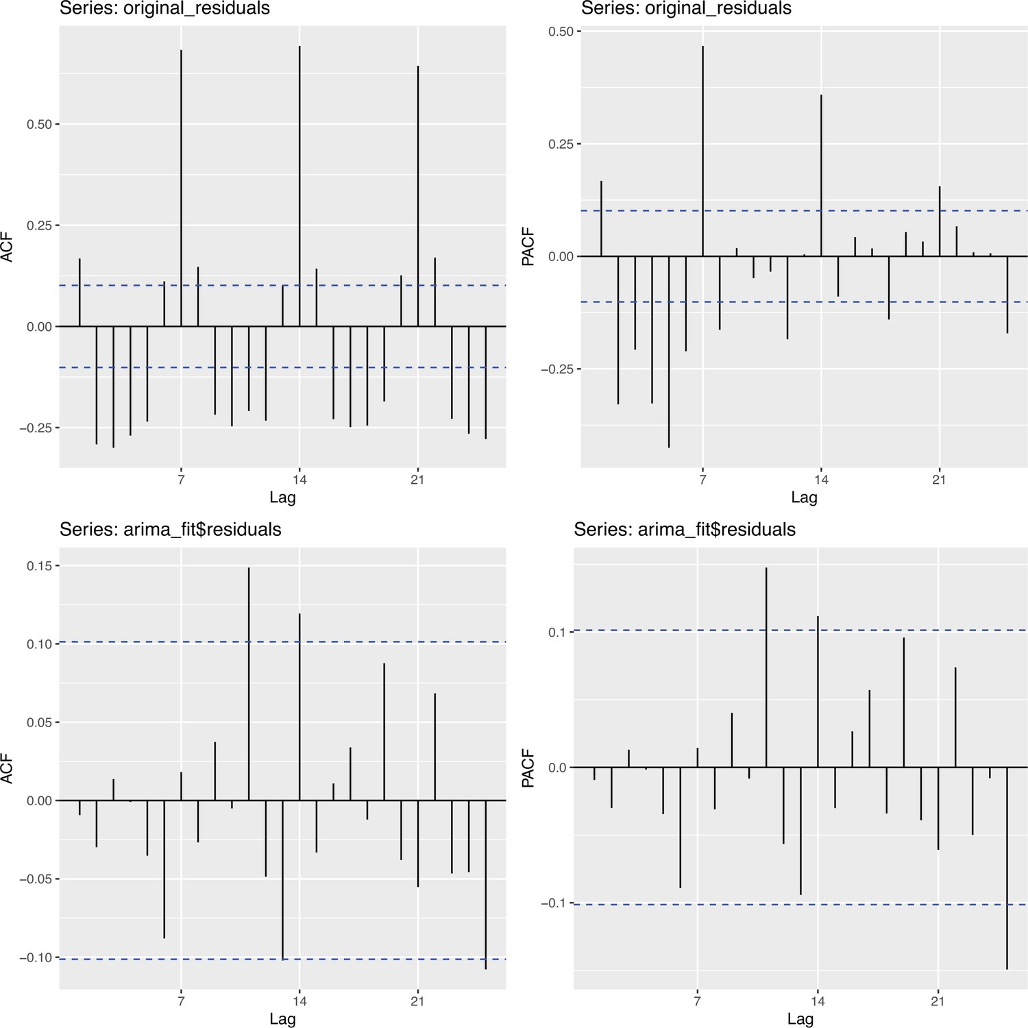
Autocorrelation function (ACF) and partial autocorrelation function (PACF) plots of observations from Switzerland and the fitted ARIMA model.

The two plots on the upper row are the ACF and PACF plots of the observations from Switzerland. The two plots on the lower row are the ACF and PACF plots of the residuals of the fitted ARIMA model.

Appendix 5—figure 4

Download asset Open asset

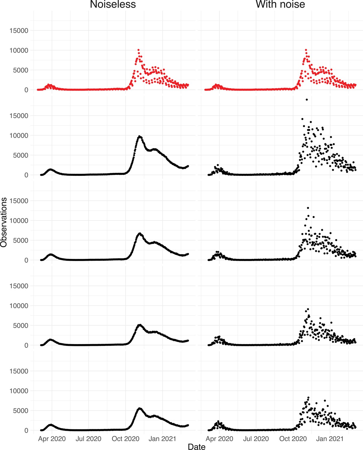
Simulated observations with and without noise.

The upper row shows the real observations from Switzerland (twice the same). The other four rows show simulated observations, the left column shows simulations without the noise term ( ${\tilde{D}}_{t}$ in Section 4.7), and the right the simulated observations with the noise term ( $D_{t}$ in Section 4.7).

Appendix 5—figure 5

Download asset Open asset

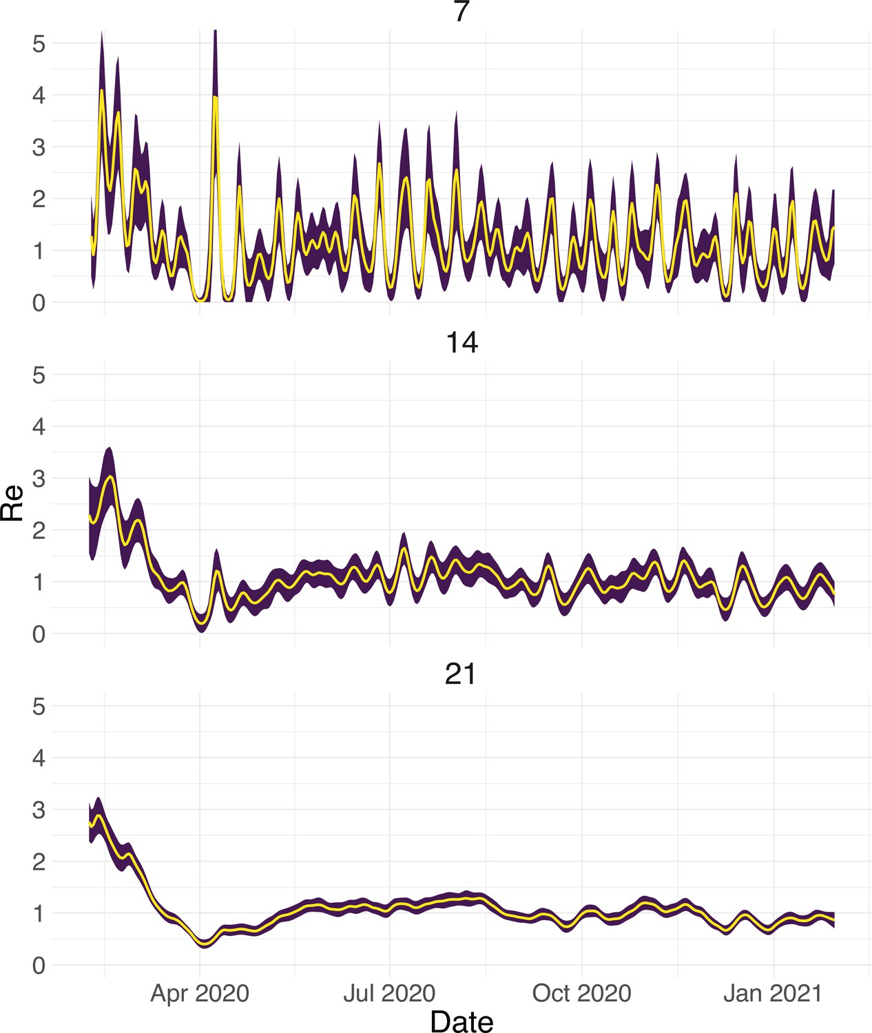
Estimated $R_{e}$ with different smoothing windows.

For each trajectory the point estimate is shown with a yellow line, and the purple ribbon indicates the 95% confidence interval.

Appendix 5—figure 6

Download asset Open asset

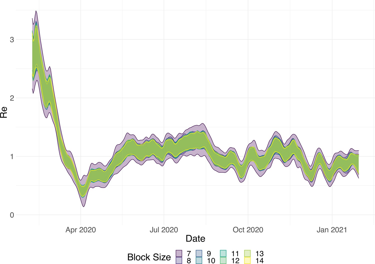
Estimated $R_{e}$ with different block sizes.

The ribbons indicate the 95% confidence interval.

Tables

Table 1

Investigating the relation between the date of ‘lockdown’ and the date when the estimated $R_{e}$ based on case reports dropped below 1.

Based on news reports, we report when a country implemented stay-at-home orders (a ‘lockdown’). The column ‘ ${\hat{R}}_{e} < 1$ ’ indicates when the $R_{e}$ point estimate first dropped below 1. The column ‘CI includes 1’ details the corresponding time interval where the 95% confidence interval included 1. Of the investigated countries that implemented a nationwide lockdown, four (Denmark, Germany, the Netherlands, Slovenia) had 95% confidence intervals that included 1 or were below before a nationwide lockdown was implemented. The column ‘Time until ${\hat{R}}_{e} < 1$ ’ indicates the number of days between the lockdown and the date that the $R_{e}$ point estimate dropped below 1.

Country	Lockdown	Re <1	CI includes 1	Time until Re <1
Austria	16–30	20–30	[20-03, 20-03]	4 days
Belgium	18–30	30–30	[25-03, 03-04]	12 days
Denmark	18–30	≤10–03	[≤10–03, 20–06]	–8 days
Finland	16–30	01-Feb	[29-03, 30-04]	17 days
France	17–30	27–30	[23-03, 07-04]	10 days
Germany	22–30	18–30	[17-03, 19-03]	–4 days
Ireland	27–30	01–100	[04–04, 15–04]	12 days
Italy	01–300	18–30	[17-03, 19-03]	8 days
Netherlands	23–30	01-Jan	[22-03, 10-04]	13 days
Norway	14–30	21–30	[17-03, 19-03]	7 days
Poland	25–30	01-Jan	[31-03, 17-04]	8 days
Portugal	16–30	28–30	[23-03, 15-04]	12 days
Romania	24–30	01-Jun	[31-03, 29-04]	13 days
Russian Federation	30–30	01-Apr	[01–05, 08–05]	35 days
Slovenia	20–30	23–30	[≤13–03, 26–03]	3 days
Spain	14–30	26–30	[25-03, 26-03]	12 days
Sweden		01-Jan	[06–03,≥03-05-2021]
Switzerland	17–30	22–30	[20-03, 22-03]	5 days
Turkey	21–30	01-Aug	[01–04, 13–04]	18 days
United Kingdom	24–30	30–30	[28-03, 20-04]	6 days

Table 2

Gamma distributions used in the pipeline: serial interval, incubation period, and the delay distributions assumed for each observation type.

Distribution	Mean (days)	SD (days)	Reference
Serial interval	4.8	2.3	Nishiura et al., 2020
Infection to onset of symptoms	5.3	3.2	Linton et al., 2020
Onset of symptoms to case confirmation	5.5	3.8	Bi et al., 2020
Onset of symptoms to hospital admission	5.1	4.2	Pellis et al., 2021
Onset of symptoms to death	15.0	6.9	Linton et al., 2020

Appendix 2—table 1

The effect of smoothing on the ability to estimate when $R_{e} = 1$ .

These values were calculated using Equation 11.

R₀	R₁	$R_{t p}$	$a_{t p}$ (per day)	Delays (days)
6.0	0.0	3.0	–0.30	6.7
3.0	0.0	1.5	–0.15	3.3
3.5	0.5	2.0	–0.15	6.7
2.5	0.5	1.5	–0.10	5.0
3.3	0.9	2.1	–0.12	9.2
1.8	0.8	1.3	–0.05	6.0

Appendix 2—table 2

Residuals and their corresponding days of the week.

Day of the week	Mon	Tue	Wed	Thu	Fri	Sat	Sun
Residuals		e₁	e₂	e₃	e₄	e₅	e₆
	e₇	e₈	e₉	e₁₀	e₁₁	e₁₂	e₁₃
	e₁₄	e₁₅	e₁₆	e₁₇	e₁₈	e₁₉	e₂₀
	e₂₁	e₂₂	e₂₃	e₂₄	e₂₅	e₂₆	e₂₇
	e₂₈	e₂₉	e₃₀

Appendix 6—table 1

Investigating the relation between the date of ‘lockdown’ and the date that the estimated $R_{e}$ dropped below 1.

The first three columns contain the same information as the first four columns of the main text Table 1. The last two columns are analogous to the third (‘ ${\hat{R}}_{e} < 1$ based on confirmed cases’) but are based on $R_{e}$ estimates for hospitalisations and deaths respectively. For each of these observation types, we used our method to determine when the $R_{e}$ estimate first dropped below 1, and for which dates the corresponding 95% confidence interval contained 1. Further, we used news reports to determine when a country implemented stay-at-home orders (a ‘lockdown’). Based on our $R_{e}$ estimates for confirmed cases, Denmark, Germany, the Netherlands, and Slovenia had 95% confidence intervals that included or were below one before a nationwide lockdown was implemented. For $R_{e}$ estimates based on COVID-19 deaths, there are also four: Denmark, the Netherlands, Poland, and the United Kingdom. See Appendix 2 for smoothing related caveats.

Country	Lockdown	${\hat{R}}_{e} < 1$ based on Confirmed cases	${\hat{R}}_{e} < 1$ based on Deaths	${\hat{R}}_{e} < 1$ based on Hospitalisations
Austria	16–03	20–03 [20-03, 20-03]
Belgium	18–03	30–03 [25-03, 03-04]	26–03 [24-03, 26-03]	25–03 [24-03, 25-03]
Denmark	18–03	10–03 [10-03, 20-06]	22–03 [18-03, 07-01]
Finland	16–03	02–04 [29-03, 30-04]	07–04 [25-03, 11-04]
France	17–03	27–03 [23-03, 07-04]	24–03 [22-03, 26-03]	27–03 [25-03, 26-03]
Germany	22–03	18–03 [17-03, 19-03]	31–03 [23-03, 04-04]
Ireland	27–03	08–04 [04–04, 15–04]	05–04 [31-03, 09-04]	06–04 [06–04, 26–04]
Italy	10–03	18–03 [17-03, 19-03]	14–03 [01–03, 29–05]
Netherlands	23–03	05–04 [22-03, 10-04]	22–03 [19-03, 02-04]	26–03 [24-03, 26-03]
Norway	14–03	21–03 [17-03, 24-03]	25–03 [18-03, 08-04]
Poland	25–03	02–04 [31-03, 17-04]	09–04 [24-03, 01-12]
Portugal	16–03	28–03 [23-03, 15-04]	28–03 [21-03, 12-04]
Romania	24–03	06–04 [31-03, 29-04]	17–04 [25-03, 28-04]
Russian Federation	30–03	04–05 [01–05, 08–05]	18–05 [14-05, 12-12]
Slovenia	20–03	23–03 [13-03, 26-03]	26–03 [20–03, ≥03-05-2021]
Spain	14–03	26–03 [25-03, 26-03]
Sweden		01–04 [06–03,≥03-05-2021]	05–04 [13–03,≥03-05-2021]
Switzerland	17–03	22–03 [20-03, 22-03]	21–03 [18-03, 23-03]	18–03 [16-03, 18-03]
Turkey	21–03	08–04 [01–04, 13–04]	04–04 [31-03, 06-04]
United Kingdom	24–03	30–03 [28-03, 20-04]	25–03 [24-03, 25-03]	29–03 [27-03, 29-03]

Appendix 6—table 2

News and public resources used to determine when a country implemented the first non-pharmaceutical interventions, and a nationwide lockdown.

Country	First Measure	Lockdown	URL
Austria	10–03	16–03	https://mrc-ide.github.io/covid19estimates/#/interventions
Belgium	10–03	18–03	https://mrc-ide.github.io/covid19estimates/#/interventions
Denmark	12–03	18–03	https://mrc-ide.github.io/covid19estimates/#/interventions
Finland	16–03	16–03	https://en.wikipedia.org/wiki/COVID-19_pandemic_in_Finland#Response_by_sector
France	29–02	17–03	https://www.politico.eu/article/europes-coronavirus-lockdown-measures-compared/
Germany	06–03	22–03	https://www.bundesregierung.de/breg-de/themen/coronavirus/besprechung-der-bundeskanzlerin-mit-den-regierungschefinnen-und-regierungschefs-der-laender-1733248
Ireland	12–03	27–03	https://en.wikipedia.org/wiki/COVID-19_pandemic_in_the_Republic_of_Ireland#Containment_phase
Italy	22–02	10–03	https://www.politico.eu/article/europes-coronavirus-lockdown-measures-compared/
Netherlands	10–03	23–03	https://www.volkskrant.nl/nieuws-achtergrond/bijeenkomsten-tot-1-juni-verboden-burgemeesters-mogen-handhaven-met-forse-boetes~b41b8508/
Norway	12–03	14–03	https://www.euractiv.com/section/coronavirus/short_news/norway-update-covid-19/
Poland	09–03	25–03	https://www.politico.eu/article/europes-coronavirus-lockdown-measures-compared/
Portugal	11–03	16–03	https://www.politico.eu/article/europes-coronavirus-lockdown-measures-compared/
Romania	21–02	24–03	https://en.wikipedia.org/wiki/COVID-19_pandemic_in_Romania
Russian Federation	25–03	30–03	https://en.wikipedia.org/wiki/COVID-19_pandemic_in_Russia
Slovenia	09–03	20–03	https://en.wikipedia.org/wiki/COVID-19_pandemic_in_Slovenia
Spain	10–03	14–03	https://www.elmundo.es/espana/2020/03/13/5e6b844e21efa0dd258b45a5.html
Sweden	11–03
Switzerland	28–02	17–03	‘Verordnung 2 über Massnahmen zur Bekämpfung des Coronavirus (COVID-19)’
Turkey	12–03	21–03	https://en.wikipedia.org/wiki/COVID-19_pandemic_in_Turkey#Government_response
United Kingdom	12–03	24–03	https://www.bbc.com/news/uk-52012432

Additional files

Supplementary file 1 A table summarising the sources of incidence data.: https://cdn.elifesciences.org/articles/71345/elife-71345-supp1-v2.xlsx
Download elife-71345-supp1-v2.xlsx
Supplementary file 2 A table comparing the structure and features of different methods to estimate Re.: https://cdn.elifesciences.org/articles/71345/elife-71345-supp2-v2.xlsx
Download elife-71345-supp2-v2.xlsx
Transparent reporting form: https://cdn.elifesciences.org/articles/71345/elife-71345-transrepform1-v2.pdf
Download elife-71345-transrepform1-v2.pdf

Download links

A two-part list of links to download the article, or parts of the article, in various formats.

Downloads (link to download the article as PDF)

Article PDF

Open citations (links to open the citations from this article in various online reference manager services)

Mendeley

Cite this article (links to download the citations from this article in formats compatible with various reference manager tools)

Jana S Huisman
Jérémie Scire
Daniel C Angst
Jinzhou Li
Richard A Neher
Marloes H Maathuis
Sebastian Bonhoeffer
Tanja Stadler

(2022)

Estimation and worldwide monitoring of the effective reproductive number of SARS-CoV-2

eLife 11:e71345.

https://doi.org/10.7554/eLife.71345

Share this article

Cite this article

Evaluation of the pipeline on simulated data.

Stability of the Swiss Re estimates based on confirmed COVID-19 cases, upon adding additional days of observations.

Comparison of published Re estimates for three countries.

Example panels from the online dashboard.

The association between the implementation or lifting of non-pharmaceutical interventions and changes in Re until May 2021.

Schematic of the effect of smoothing on the ability to estimate when Re=1.

Performance of our method on simulated scenarios with differing slopes.

Performance of our method, modified to skip the smoothing step in the pipeline, on simulated scenarios with observation noise.

Performance of our method on simulated scenarios with observation noise.

Performance of our method on simulated scenarios with varying population size, using confidence intervals from EpiEstim.

Performance of our method on simulated scenarios with varying population size, using the Union of EpiEstim and Block bootstrap 95% confidence intervals.

Performance of our method on simulated scenarios using a fixed shift versus the deconvolution to infer infection incidence.

Performance of our method on simulated scenarios with misspecified delay distributions.

Performance of our method on simulated scenarios with time-varying delay distributions.

Stability of Re estimates at present.

Mean delay in Switzerland between onset of symptoms and reporting.

Comparison of the Re estimates with or without accounting for known symptom onset dates and for time-variability on reporting delays.

Effective reproductive number estimates with or without accounting for known imports.

Square root and log transformations to stabilise the variance of residuals.

Autocorrelation function (ACF) and partial autocorrelation function (PACF) plots of the observations from five different countries.

Autocorrelation function (ACF) and partial autocorrelation function (PACF) plots of observations from Switzerland and the fitted ARIMA model.

Simulated observations with and without noise.

Estimated Re with different smoothing windows.

Estimated Re with different block sizes.

Investigating the relation between the date of ‘lockdown’ and the date when the estimated Re based on case reports dropped below 1.

Gamma distributions used in the pipeline: serial interval, incubation period, and the delay distributions assumed for each observation type.

The effect of smoothing on the ability to estimate when Re=1.

Residuals and their corresponding days of the week.

Investigating the relation between the date of ‘lockdown’ and the date that the estimated Re dropped below 1.

News and public resources used to determine when a country implemented the first non-pharmaceutical interventions, and a nationwide lockdown.

Supplementary file 1

Supplementary file 2

Transparent reporting form

Downloads (link to download the article as PDF)

Open citations (links to open the citations from this article in various online reference manager services)

Cite this article (links to download the citations from this article in formats compatible with various reference manager tools)

Stability of the Swiss $R_{e}$ estimates based on confirmed COVID-19 cases, upon adding additional days of observations.

Comparison of published $R_{e}$ estimates for three countries.

The association between the implementation or lifting of non-pharmaceutical interventions and changes in $R_{e}$ until May 2021.

Schematic of the effect of smoothing on the ability to estimate when $R_{e} = 1$ .

Stability of $R_{e}$ estimates at present.

Comparison of the $R_{e}$ estimates with or without accounting for known symptom onset dates and for time-variability on reporting delays.

Estimated $R_{e}$ with different smoothing windows.

Estimated $R_{e}$ with different block sizes.

Investigating the relation between the date of ‘lockdown’ and the date when the estimated $R_{e}$ based on case reports dropped below 1.

The effect of smoothing on the ability to estimate when $R_{e} = 1$ .

Investigating the relation between the date of ‘lockdown’ and the date that the estimated $R_{e}$ dropped below 1.