Empirical single-cell tracking and cell-fate simulation reveal dual roles of p53 in tumor suppression
Figures
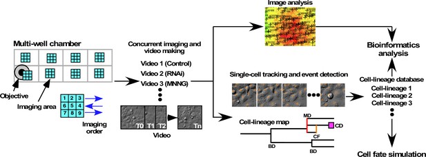
System for investigating the functional role of maintaining low cell levels of p53.
A549 cells were cultured on multi-well chamber slides and the areas of interest were scanned. Cells were treated with scrambled siRNA or p53 siRNA in the presence or absence of various doses of MNNG, and the cell responses were monitored to generate live-cell imaging videos. The videos were used for imaging and single-cell tracking, starting immediately after MNNG treatment. Progenitors were selected from the image designated as tracking time 0 min (T0), and the progenitors and their progeny were tracked empirically. Cell-lineage database comprised tracking results for one progenitor and their progeny, and any events that occurred in the cells. A cell-lineage map was generated from the database to represent the proliferation profile of a progenitor and its progeny through bipolar cell division (BD), multipolar cell division (MD), cell fusion (CF), and cell death (CD). If any progeny moved out from the areas of interest, data related to the lineage of that was not included in the cell-lineage database. Quantitative bioinformatics analysis was performed using the database, which was also used to develop a cell-fate simulation algorithm.
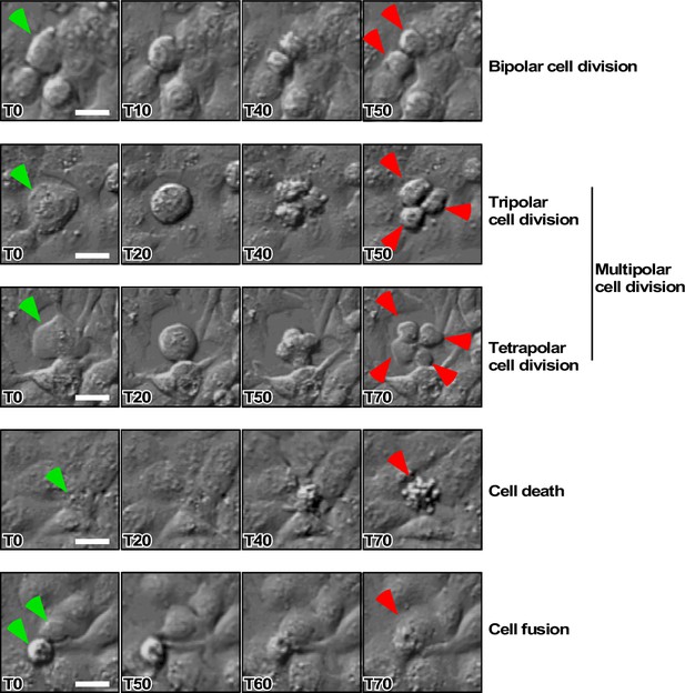
Events occurring in the cells.
Cellular events that occurred in A459 cells were categorized as follows: bipolar cell division, tripolar cell division, tetrapolar cell division, cell death, and cell fusion. In this study, tripolar and tetrapolar cell divisions were defined as multipolar cell division. Green arrowheads indicate cells that underwent an event. Red arrowheads indicate daughter cells, a dead cell, and a fused cell. Timestamps (min) relative to the first frame and a scale bar (20 μm) are shown. Corresponding videos are deposited in Dryad.
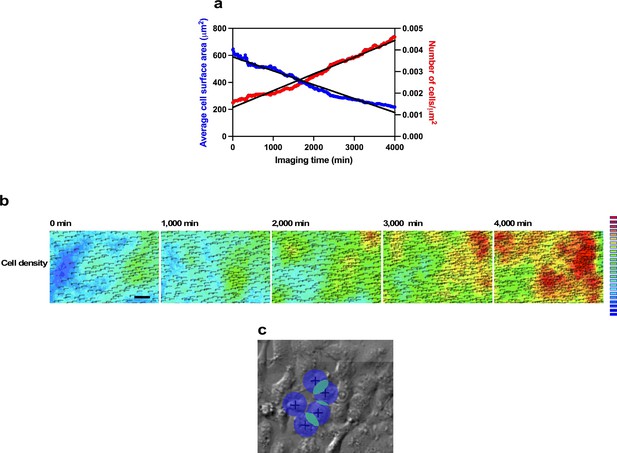
Quantitation of cell numbers, areas, and densities.
(a) Cell density and average cell size were plotted every 10 min. (b) Cell density maps were created using a heat map scale. Still images were taken from Figure 1—video 1. Timestamps (min) and a scale bar (80 μm) are shown. (c) The cell positions that were determined using single-cell tracking and recorded in the cell-lineage database were used. Cell density map created by assigning value 1 to a pixel within the 20-pixel diameter area from the position of a cell (blue); if an area overlapped with other areas, the pixel was assigned the sum of the number of overlapped areas (light green). At the high cell density area, values were increased according to the number of overlaps, allowing to generate a heat map. These values were used to generate heat maps.
-
Figure 1—figure supplement 2—source data 1
Quantitation of cell numbers, areas, and densities.
Data used in Figure 1—figure supplement 2.
- https://cdn.elifesciences.org/articles/72498/elife-72498-fig1-figsupp2-data1-v3.xlsx
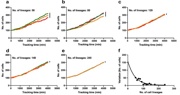
Determination of minimum number of cell-lineages required to build a cell-lineage database.
A cell-lineage database containing 50–240 cell lineages was used to determine cell population expansion curves. Cell-lineage database was created by tracking of 485 progenitors of Control cells. (a–e) Cell population expansion curves determined by randomly selecting 50 (a), 80 (b), 120 (c), 140 (d), and 240 (e) cell lineages from the cell-lineage database. The number of cells every 10 min was calculated and plotted. The random selection was repeated three times (green, orange, and red lines) to show variations at a tracking time of 4000 min (black bars). Each repeated selection was performed in a way that the same lineage was not selected, except for the selection of 240 lineages. The initial number of cell lineages was normalized to 100. (f) Variations of 4000 min are plotted.
-
Figure 1—figure supplement 3—source data 1
Determination of minimum number of cell lineages required to build a cell-lineage database.
Data used in Figure 1—figure supplement 3.
- https://cdn.elifesciences.org/articles/72498/elife-72498-fig1-figsupp3-data1-v3.xlsx
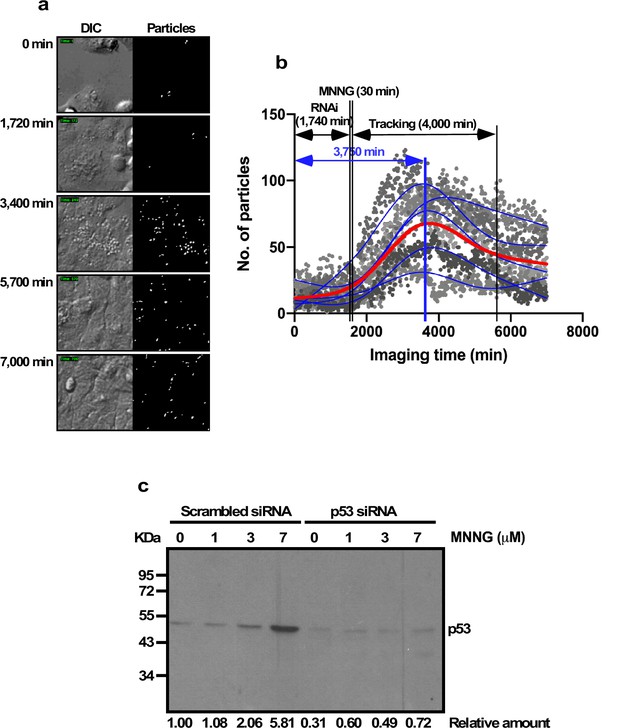
Accumulation of particles following siRNA transfection and analysis of p53 expression following transfection and/or MNNG exposure.
(a) Particles formed following siRNA transfection are shown. DIC and objects with pixel value 150–254 and size 5–30 pixels were extracted from the DIC image (Particles). (b) The numbers of particles at five different locations in the image are plotted. Blue lines represent the average number of particles at each time point per location, and the red line shows the overall average. MNNG treatment was performed after approximately 1740 min of siRNA transfection and continued for 30 min. The number of particles peaked at 3750 min after transfection. Single-cell tracking was started immediately after MNNG treatment and continued for 4000 min. (c) Western blotting with anti-p53 antibody was performed 48 hr after siRNA treatment. Amounts of p53 relative to Control are shown.
-
Figure 1—figure supplement 4—source data 1
Accumulation of particles following siRNA transfection and analysis of p53 expression following transfection and/or MNNG exposure.
Data used in Figure 1—figure supplement 4.
- https://cdn.elifesciences.org/articles/72498/elife-72498-fig1-figsupp4-data1-v3.xlsx
Visualization of cell density.
Density of cultured cells visualized using a heat map color scale. Timestamps (min) and a scale bar (80 μm) are shown.
Visualization of progress of transfection.
DIC and particles with 150–255 grayscale and size of 5–30 pixels are shown. Timestamps (min) and a scale bar (20 μm) are shown.
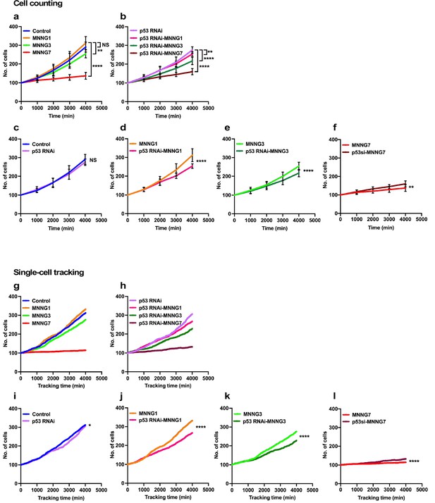
Cell population expansion rates determined by cell-counting and single-cell-tracking analysis.
Control (a) and p53 RNAi (b) cells were exposed to 1, 3, and 7 µM MNNG (Control and p53 RNAi cells exposed to those doses of MNNG are referred to as MNNG1, MNNG3, MNNG7, p53 RNAi-MNNG1, p53 RNAi-MNNG3, and p53 RNAi-MNNG7, respectively). (a–f) Images were divided into a 5 × 5 squares and cell population expansion curves were determined by counting the number of cells in a square (~512 × 512 pixels) at 1000 min intervals (see Figure 2—figure supplement 1). Fifteen squares were selected from three independently generated videos. Expansion curves were compared as follows: Control vs. p53 RNAi (c), MNNG1 vs. p53 RNAi-MNNG1 (d), MNNG3 vs. p53 RNAi-MNNG3 (e), and MNNG7 vs. p53 RNAi-MNNG7 (f) cells. Student’s t-test (c–f) and ordinary one-way ANOVA (Tukey’s) (a, b) were performed (n = 15), and standard errors are shown. Cell population expansion curves of Control (g) and p53 RNAi (h) cells were determined using a cell-lineage database. Single-cell tracking was performed for 4000 min with videos acquired at 10 min intervals (n = 399). The number of cells every 10 min was extracted and plotted. Cell population expansion curves were compared as follows: Control vs. p53 RNAi (i), MNNG1 vs. p53 RNAi-MNNG1 (j), MNNG3 vs. p53 RNAi-MNNG3 (k), and MNNG7 vs. p53 RNAi-MNNG7 (l) cells. (i–l) The data were analyzed by Student’s t-tests in the following approach. The difference in cell numbers between n and n + 10 min was calculated (e.g., if the numbers of cells at 10 and 20 min were 100 and 103, the difference was 3). Because the total number of imaging points was 400, the 399 differences in time points can be calculated. Those differences for Control and p53 RNAi cells and those exposed to MNNG were used for the statistical analyses. (a–f, i–l) NS, nonsignificant, *p<0.05, **p<0.01, ***p<0.001, ****p<0.0001.
-
Figure 2—source data 1
Cell population expansion rates determined by cell-counting and single-cell-tracking analysis.
Data used in Figure 2.
- https://cdn.elifesciences.org/articles/72498/elife-72498-fig2-data1-v3.xlsx
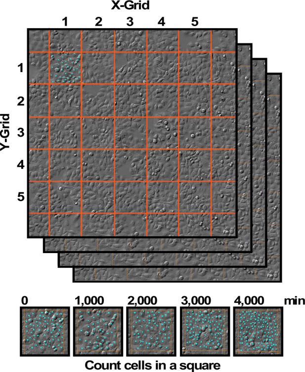
Determination of cell population expansion rate using video images.
A video image (typically 2560 pixels × 2560 pixels) was divided into 5 × 5 squares and the numbers of cells in selected squares were counted. Counting was performed every 1000 min in video images from 0 to 4000 min.
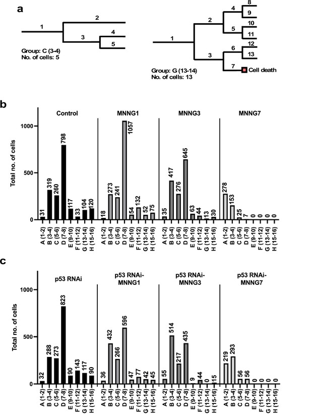
Number of progeny produced from a progenitor.
(a) Example cell lineages are shown. If a cell lineage was composed of one progenitor (1) and four progenies (2–5) (a: left), the cell lineage was grouped as C (5–6). Similarly, if a cell lineage was composed of one progenitor (1) and 12 progenies (2–13) (b: right), the lineage was grouped as G (13–14). Cells that underwent multipolar cell division, cell death, and cell fusion were also included in this analysis. (b, c) The total number of cells belonging to each group was calculated. For example, if five cell lineages were composed of three cells (group B), the number of cells in group B was 5 × 3 = 15, which could represent the number of cells with the reproductive ability to produce three cells within 4000 min of culture in a cell population. (b) Control cells and cells exposed to MNNG. (c) p53 RNAi cells and cells exposed to MNNG.
-
Figure 3—source data 1
Number of progeny produced from a progenitor.
Data used in Figure 3.
- https://cdn.elifesciences.org/articles/72498/elife-72498-fig3-data1-v3.xlsx
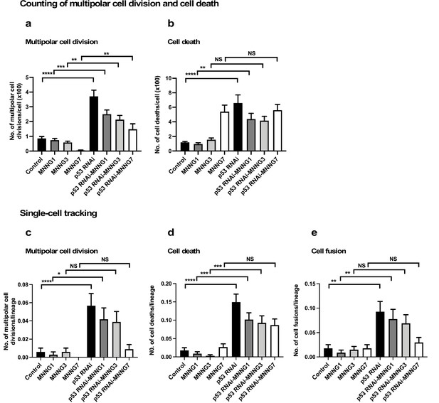
Analysis of multipolar cell division, cell death, and cell fusion using counting and single-cell-tracking analysis.
Control and p53 RNAi cells were exposed to 1, 3, and 7 µM MNNG. The numbers of multipolar cell division (a) and cell death (b) events that occurred during the tracking time (4000 min) were determined by counting those events recorded in a video. Each time point of image was divided into four areas (Figure 4—figure supplement 1), and three independently generated videos were used. Thus, counting was performed in 12 squares (n = 12). The numbers of multipolar cell division (c), cell death (d), and cell fusion (e) events that occurred during the tracking time (4000 min) were determined using single-cell-tracking and cell-lineage database (n = 335). (a–e) Statistical analysis was performed by ordinary one-way ANOVA (Tukey’s). NS, non-significant, *p<0.05, **p<0.01, ***p<0.001, ****p<0.0001. Standard errors are shown.
-
Figure 4—source data 1
Analysis of multipolar cell division, cell death, and cell fusion using counting and single-cell-tracking analysis.
Data used in Figure 4.
- https://cdn.elifesciences.org/articles/72498/elife-72498-fig4-data1-v3.xlsx
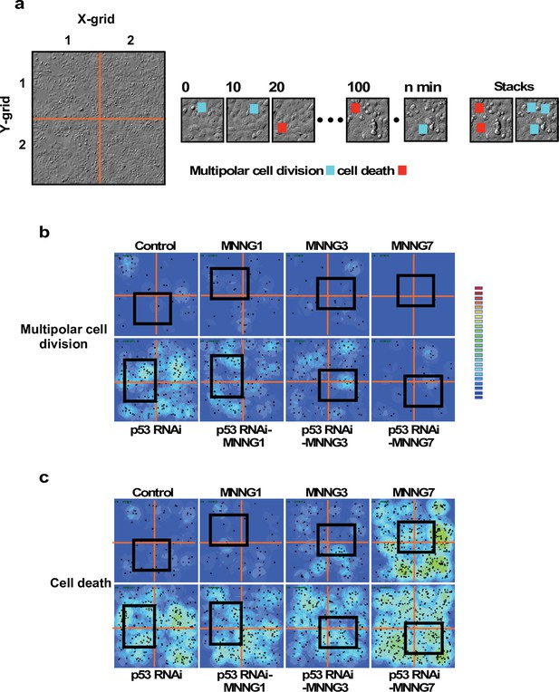
Counting multipolar cell division and cell death using live-cell imaging videos.
(a) Each time point of the video image was divided into four squares, and cell death and multipolar cell division in each square were marked to determine the numbers of those events that occurred during imaging. Three independently generated videos were used, and total 12 squares were thus counted. The positions of multipolar cell division and cell death were also stacked to generate multipolar cell division and cell death density maps. Multipolar cell division (b) and cell death (c) density maps were created using a similar approach to cell density determination (Figure 1—figure supplement 2b). Density is shown using a heat map scale. Black squares correspond to the area used for single-cell tracking.
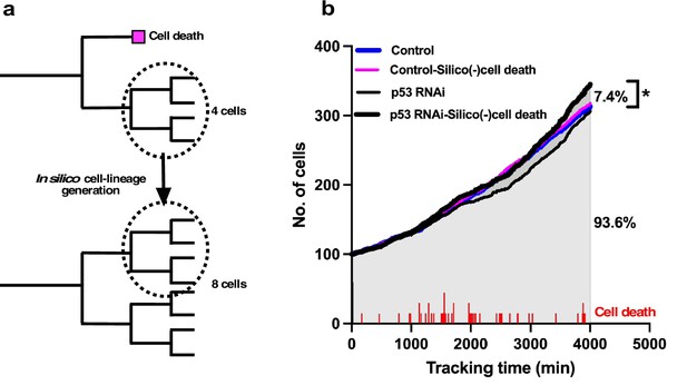
In silico generation of cell-lineage database to evaluate the impact of cell death on the cell population expansion.
(a) To evaluate the impact of cell death on population expansion, we created an in silico cell-lineage database, in which cells do not undergo cell death, to address the impact of cell death on the cell population expansion. In the example cell lineages, the number of survived cells was reduced by half as a result of cell death. If the siblings of the dead cell grew, the dead cell was assumed to continue to grow similar to its sibling, and a cell-lineage database was created in silico based on this assumption. (b) A cell population expansion curve was generated using the in silico-created cell-lineage database for Control and p53 RNAi cells (Control-Silico(-)cell death and p53 RNAi-Silico(-)cell death, respectively). At a tracking time of 4000 min, cell death resulted in a 7.4% reduction in the population size of p53 RNAi cells. The frequency of cell death (red lines) occurring during tracking is also shown. Statistical analysis was performed by ordinary one-way ANOVA (Tukey’s). *p<0.05.
-
Figure 5—source data 1
In silico generation of cell-lineage database to evaluate the impact of cell death on cell population expansion.
Data used in Figure 5.
- https://cdn.elifesciences.org/articles/72498/elife-72498-fig5-data1-v3.xlsx
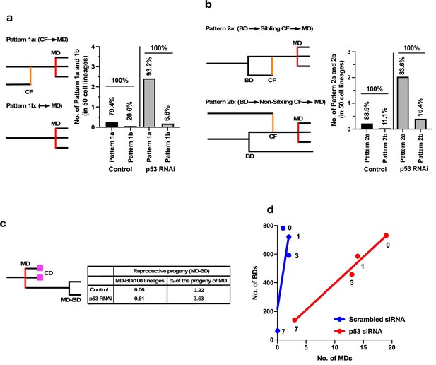
Events leading to the induction of multipolar cell division.
(a) Cellular events that occurred prior to multipolar cell division were analyzed by tracing the cell lineage backward. Pattern 1a (cell fusion [CF] ➛ multipolar cell division [MD]): cell fusion occurred prior to multipolar cell division. Pattern 1b (➛ MD): no cell fusion occurred. The numbers of each pattern occurring in 50 cell lineages are shown. Percentages of Patterns 1a and 1b in Control and p53 RNAi cells are also shown. (b) Cells that underwent multipolar cell division were identified. If the cells were generated by cell fusion, the origin of the fused cells was searched by tracing the cell lineage backward. Pattern 2a (BD ➛ sibling CF ➛ MD): bipolar cell division occurred, cells produced by division were fused, followed by multipolar cell division. Pattern 2b (BD ➛ non-sibling CF ➛ MD): one sibling produced by bipolar cell division was fused with another non-sibling cell, followed by multipolar cell division. The numbers of each pattern in 50 cell lineages are shown. Percentages of Patterns 2a and 2b in Control and p53 RNAi cells are also shown. (c) Progeny produced by multipolar cell division was tracked and the number of reproductive progeny that underwent bipolar cell division was determined. The numbers of reproductive progeny found in 100 cell lineages and the percentages of such progeny among the total number of progeny produced by multipolar cell divisions are shown. (d) The number of multipolar cell division events was plotted against the number of bipolar cell division events. Numbers in (d) indicate doses of MNNG. (a–d) Because the number of multipolar cell divisions in Control cells was low, we searched three videos to find multipolar cell divisions and then traced the cells back to their progenitors to determine the events preceding multipolar cell division. To normalize the values, we assumed that multipolar cell division occurred at a similar frequency to that recorded in the cell-lineage database. BD: bipolar cell division; MD: multipolar cell division, CD: cell death; and CF: cell fusion.
-
Figure 6—source data 1
Events leading to the induction of multipolar cell division.
Data used in Figure 6.
- https://cdn.elifesciences.org/articles/72498/elife-72498-fig6-data1-v3.xlsx
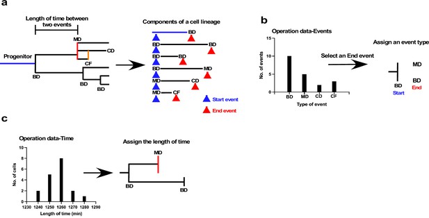
Schematic illustration of cell-fate simulation process.
(a) A cell lineage is composed of a progenitor and its progeny. Each of those cells is generated by a Start event (blue arrowhead), followed after a certain length of time by an End event (red arrowhead), such as bipolar cell division (BD), multipolar cell division (MD), cell death (CD), and cell fusion (CF). Cell-fate simulation was performed by combining these components, types of event, and length of time between the two events. To perform the simulation, cells were classified based on the combination of the Start and the End events; for example, BD-BD, and BD-MD (see Figure 7—figure supplement 2 for full list of classifications), and two sets of histogram data, referred to as Operation data-Events and Operation data-Time, were created. (b) The Operation data-Events holds the frequency of events that occurred following a Start event, such as BD, MD, or CF. In the case of the example shown in (b), if the Start event was BD, the histogram data indicated that the chances of the occurrence of each End event type, that is, BD, MD, CD, and CF, were 10, 5, 2, and 3, respectively. In the example, MD and BD were selected from the histogram to assign an End event type to daughter cells produced by BD. Selection was performed by generating a random value. (c) Operation data-Time was then used to assign the length of time between the Start and End events using histogram data (Operation data-Time) for BD-BD and BD-MD, which included the choices of length of time. The processes were repeated to generate cell-lineage data for virtual cells.
-
Figure 7—source code 1
Single-cell tracking and cell-fate simulation processes.
(a) Overall scheme of single-cell tracking. (b) Processes of cell-fate simulation.
- https://cdn.elifesciences.org/articles/72498/elife-72498-fig7-code1-v3.docx
-
Figure 7—source code 2
Cell-fate simulation.
- https://cdn.elifesciences.org/articles/72498/elife-72498-fig7-code2-v3.docx
-
Figure 7—source code 3
Cell-fate simulation.
- https://cdn.elifesciences.org/articles/72498/elife-72498-fig7-code3-v3.docx
-
Figure 7—source code 4
Cell-fate simulation.
- https://cdn.elifesciences.org/articles/72498/elife-72498-fig7-code4-v3.docx
-
Figure 7—source code 5
Cell-fate simulation.
- https://cdn.elifesciences.org/articles/72498/elife-72498-fig7-code5-v3.docx
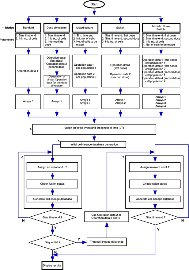
Cell-fate simulation algorithm.
Overall summary of the algorithm. Ltime (LT).
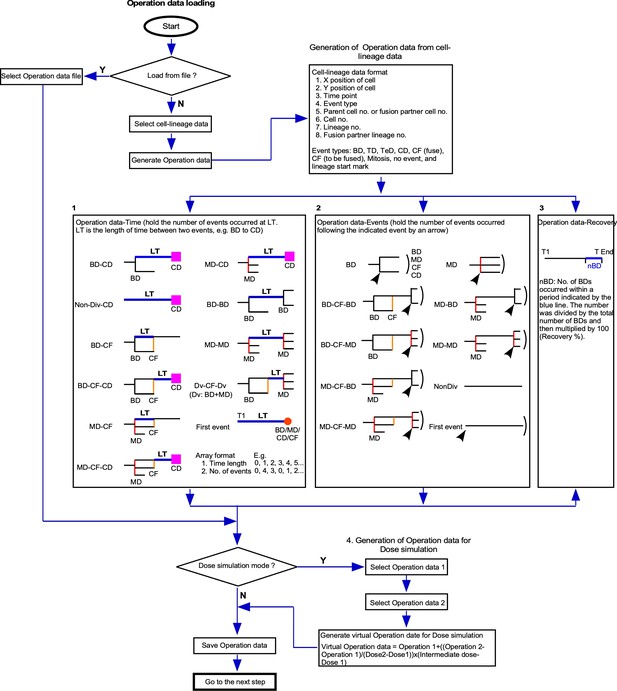
Cell-fate simulation algorithm.
Creation of Operation data and its types. Bipolar cell division (BD), multipolar cell division (MD), cell death (CD), cell fusion (CF), no cell division (NonDiv), and Ltime (LT).
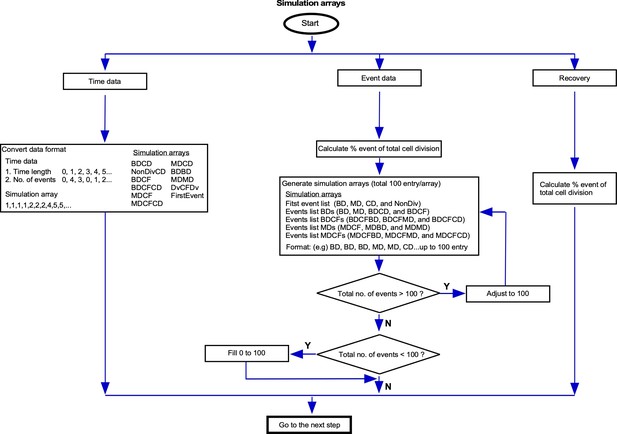
Cell-fate simulation algorithm.
Simulation arrays and its format. Bipolar cell division (BD), multipolar cell division (MD), cell death (CD), cell fusion (CF), and no cell division (NonDiv).
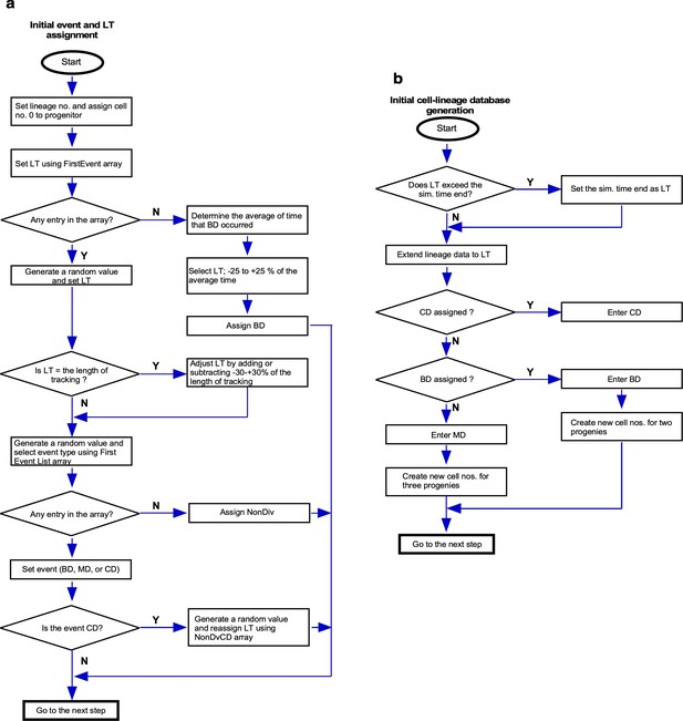
Cell-fate simulation algorithm.
(a) Initial event assignment, and (b) initial cell-lineage database generation. Bipolar cell division (BD), multipolar cell division (MD), cell death (CD), cell fusion (CF), no cell division (NonDiv), and Ltime (LT).
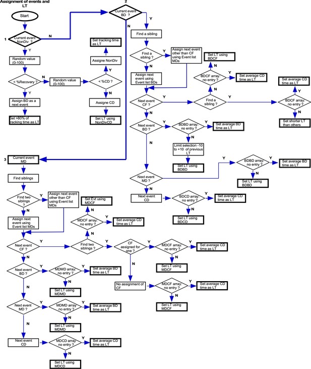
Cell-fate simulation algorithm.
Main event assignment. Bipolar cell division (BD), multipolar cell division (MD), cell death (CD), cell fusion (CF), no cell division (NonDiv), and Ltime (LT).
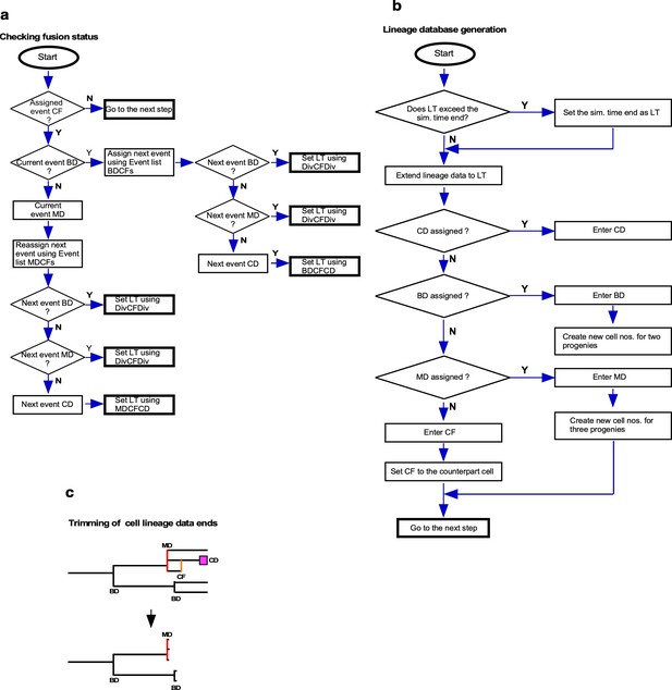
Cell-fate simulation algorithm.
(a) Re-assignment of events in cases with cell fusion, (b) cell-lineage database generation, and (c) trimming of cell-lineage data ends to switch from the first to second Operation data. Bipolar cell division (BD), multipolar cell division (MD), cell death (CD), cell fusion (CF), no cell division (NonDiv), and Ltime (LT).
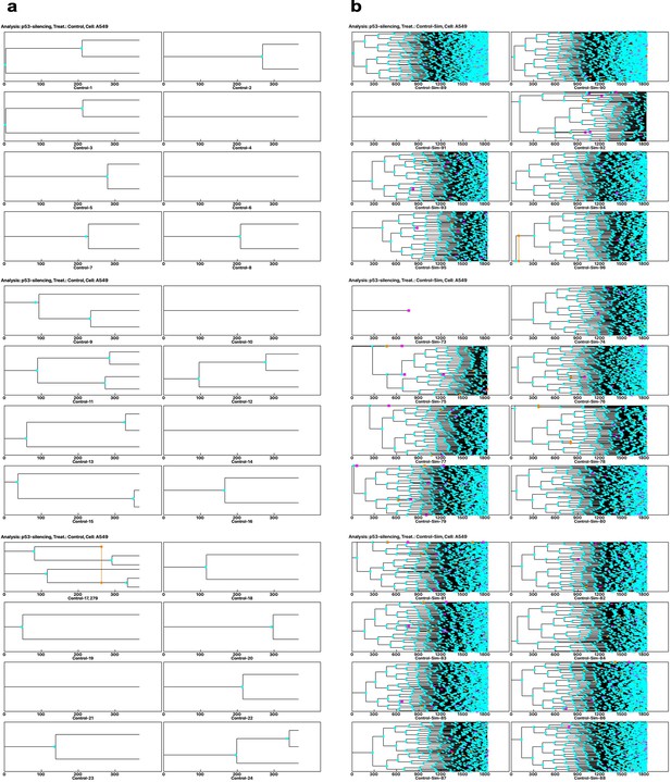
Cell-lineage maps generated by single-cell -tracking and a cell-fate simulation algorithm.
(a) Cell-lineage maps generated by cell-lineage database Control cells. The single-cell tracking analysis created 335 cell-lineage datasets,, and 16 cell-lineage maps are shown as examples. (b) Cell-lineage maps generated by simulation using Operation data-p53 RNAi. The simulation created 2,500–5,000 virtual cell-lineage datasets, and 16 cell-lineage maps generated from the virtually created cell-lineage datasets are shown as examples. Light blue circle, mitosis; pink square, cell death; orange circle and orange vertical line, cell fusion; black vertical line, bipolar cell division; red vertical line, multipolar cell division.
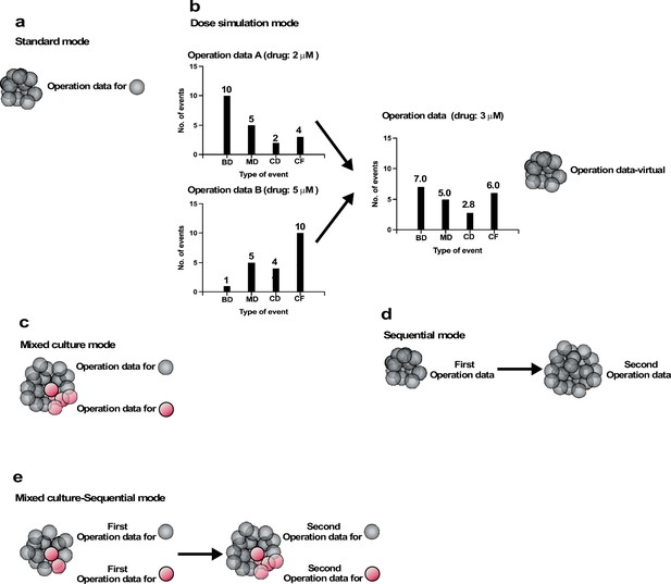
Operation modes.
(a) Standard mode: cell-fate simulation with one type of cell population performed with Operation data. (b) Dose simulation mode: Operation data created from other Operation data. The example in (b) represents an Operation data-Events, which holds information on the chance of the occurrence of subsequent events following an event, as outlined in Figure 7c. In the case of Operation data A, generated from a cell-lineage database created by tracking cells exposed to a dose of a drug (e.g., 2 µM MNNG), 10, 5, 2, and 4 bipolar cell division (BD), multipolar cell division (MD), cell death (CD), and cell fusion (CF) events, respectively, occurred following the event. On the other hand, Operation data B, generated from a cell-lineage database created by tracking cells in another cell population exposed to a different dose (e.g., 5 µM) of the drug, assumed that 1, 5, 4, and 10 BD, MD, CD, and CF events would occur following the same type of events referred to in Operation A. If a cell population was assumed to be exposed to the drug at 3 µM, Operation data for the exposed cells could be created by calculating; for example, BD (7) = BD for Operation data A (10) + [(Operation data B (1) − Operation data A (10)/(Dose 2 (×5) − Dose 1 (×2))) × (Intermediate dose (×3) − Dose 1 (×2))]. A similar calculation can be performed for all data stored in Operation data-Time and -Events to create new Operation data (Operation data-virtual). Using the Operation data, the cell fate could be simulated without the need for empirical analysis. (c) Mixed culture mode: assuming that multiple cell types coexist in a culture, simulation was performed using corresponding Operation data for each cell type. (d) Switch mode: cell-fate simulation is performed with Operation data and then switched to another Operation data. If the second Operation data is for cells treated with a drug, this simulation allow the effect of the drug treatment to be evaluated virtually. (e) Mixed culture-Switch mode: this mode is a combined Mixed culture (c) and Switch (d) mode.
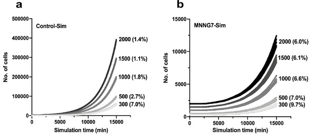
Determination of number of progenitors required to perform a reproducible simulation.
The simulation was performed with 300–2000 progenitors using either the Operation data-Control (a) or Operation data-MNNG7 (b). Each simulation was repeated five times and virtual cell-lineage databases for Control-Sim and MNNG7-Sim cells were created to determine the population expansion curves of the virtual cells. The percentage of variation relative to the average at simulation time 15,000 min is also shown in parentheses.
-
Figure 8—figure supplement 1—source data 1
Determination of number of progenitors required to perform a reproducible simulation.
Data used in Figure 8—figure supplement 1.
- https://cdn.elifesciences.org/articles/72498/elife-72498-fig8-figsupp1-data1-v3.xlsx
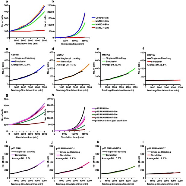
Simulations of effects of p53 silencing and MNNG exposure on cell population expansion.
Simulations were performed using Operation data generated from cell-lineage data with a total of 5000 virtual progenitors for a simulation time of 15,000 min. (a, b) Virtual cell population expansion curves of Control-Sim cells and cells exposed to various doses of MNNG (a) 0–4000 min and (b) whole scale (0–15,000 min). (c–f) Data obtained from the simulation were compared with cell population expansion curves determined by single-cell-tracking analysis; (c) Control, (d) MNNG1, (e) MNNG3, and (f) MNNG7. Difference (%) was determined by obtaining the sum of the number of cells (single-cell tracking)/the number of Simulated cells determined at each simulation time point divided by 1500 simulation time ×100. For example, a difference of 2.7% implied that the simulation generated 2.7% more cells compared with the single-cell-tracking data. (g, h) Virtual cell population expansion curves of p53 RNAi-Sim cells and cells exposed to various doses of MNNG (g) 0–4000 min and (h) whole scale (0–15,000 min). (i–l) These simulation data were compared with the cell population expansion curves determined by single-cell-tracking analysis; (i) p53 RNAi, (j) p53 RNAi-MNNG1, (k) p53 RNAi-MNNG3, and (l) p53 RNAi-MNNG7. Results of simulation obtained using Operation data-p53 RNAi-Silico(-)cell death are also included in (g) and (h).
-
Figure 9—source data 1
Simulations of effects of p53 silencing and MNNG exposure on cell population expansion.
Data used in Figure 9.
- https://cdn.elifesciences.org/articles/72498/elife-72498-fig9-data1-v3.xlsx
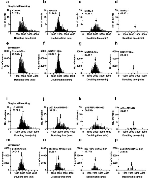
Cell-doubling time distribution.
Cell-doubling time distribution was determined using the cell-lineage database generated by single-cell-tracking and simulation data. (a–d) Cell doubling times of (a) Control, (b) MNNG1, (c) MNNG3, and (d) MNNG7 cells determined using the cell-linage database. (e–h) Simulations were performed using the Operation data (e) Control, (f) MNNG1, (g) MNNG3, and (h) MNNG7. (i–l) Cell doubling time of (i) p53 RNAi, (j) p53 RNAi-MNNG1, (k) p53 RNAi-MNNG3, and (l) p53 RNAi-MNNG7. (m–p) Results of corresponding simulations are shown; the Operation data (m) p53 RNAi, (n) p53 RNAi-MNNG1, (o) p53 RNAi-MNNG3, and (p) p53 RNAi-MNNG7. Arrow indicates the average cell-doubling time, and the average cell-doubling times are shown.
-
Figure 9—figure supplement 1—source data 1
Cell-doubling time distribution.
Data used in Figure 9—figure supplement 1.
- https://cdn.elifesciences.org/articles/72498/elife-72498-fig9-figsupp1-data1-v3.xlsx
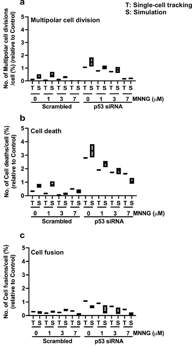
Simulation results for numbers of multipolar cell division, cell death, and cell fusion events.
The numbers of multipolar cell division (a), cell death (b), and cell fusion (c) events in a virtual cell population generated by the simulation were compared with those determined by single-cell tracking analysis. The simulation was performed with 1000 progenitors for a simulation time of 15,000 min and was repeated 10 times. The range of results obtained by the simulation is also indicated.
-
Figure 9—figure supplement 2—source data 1
Simulations of multipolar cell division, cell death, and cell fusion.
Data used in Figure 9—figure supplement 2.
- https://cdn.elifesciences.org/articles/72498/elife-72498-fig9-figsupp2-data1-v3.xlsx
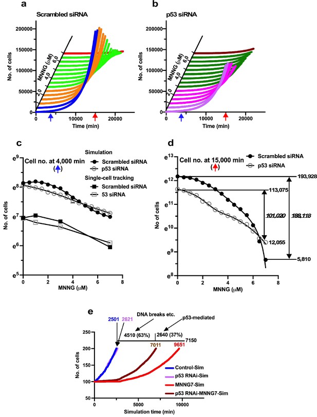
Virtual dose–response analysis.
Virtual Operation data corresponding to each 0.5 µM dose of MNNG was generated in Dose simulation mode. (a, b) Virtual MNNG-dose–response cell population expansion curves of Control and p53 RNAi cells generated by the simulation using Operation data-Control to MNNG 1.5 (purple), 2–3 (pink), 3.5–6.5 (dark green), and 7 (maroon) are shown. (c) The numbers of cells at simulation times of 4000 min (indicated by a blue arrow in a and b) are plotted. Results of single-cell-tracking analysis are also included. (d) The numbers of cells at simulation times of 15,000 min (indicated by a red arrow in a and b) are plotted. The difference of cell number between Control cells and the cells exposed to 7 μM MNNG, and p53 RNAi cells and the cells to the dose of MNNG is shown (italic). The number of cells at 0 and 15,000 min is also shown. (c, d) Standard deviations are shown. A natural log scale was used. (e) Time necessary to reach a cell population to be doubled (100–200 cells) was determined by using Operation data-Control, MNNG7, p53 RNAi, and p53 RNAi-MNNG7. The difference in time between MNNG7-Sim (9651 min) and Control-Sim (2501 min) was 7150 min. Similarly, the difference in doubling time between p53 RNAi-MNNG7-Sim and p53 RNAi-Sim was 4510 min. Assuming that the difference in doubling time between MNNG7-Sim and Control-Sim represents the effect of MNNG induced by, for example, DNA breaks and p53-mediated responses, while that between p53 RNAi-MNNG7-Sim and p53 RNAi-Sim only represents the effect of MNNG induced by, for example, DNA breaks, 63 and 37% of suppression of cell population expansion in MNNG7-Sim were likely to be due to the effect of MNNG caused by, for example, DNA breaks and responses induced by the stabilization of p53, respectively.
-
Figure 10—source data 1
Virtual dose–response analysis.
Data used in Figure 10.
- https://cdn.elifesciences.org/articles/72498/elife-72498-fig10-data1-v3.xlsx
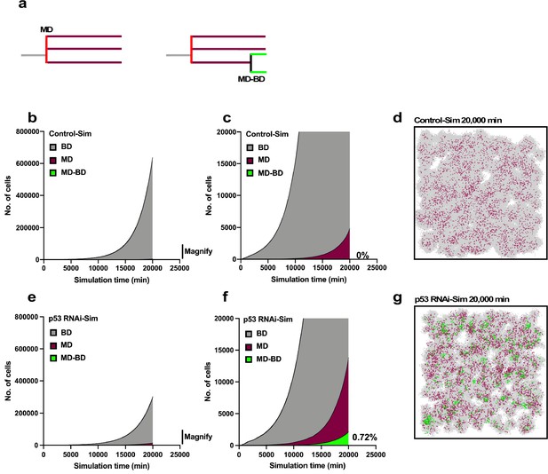
Simulation of proliferation of progeny of multipolar cell division.
The simulation was performed using Operation data-Control and p53 RNAi in Standard mode. (a) The numbers of progeny of bipolar cell division (gray), multipolar cell division (burgundy), and progeny cells that first underwent multipolar cell division followed by bipolar cell division (green) are plotted. The simulation was carried out for 2500 progeny, which generated 6.6 × 10⁶ cells during the 20,000 min of simulation. (b, c) Whole-scale and magnified images generated by the simulation using the Operation data-Control are shown in (b) and (c), respectively. (d) An animation was created to visualize the proliferation of Control-Sim cells (Figure 11—video 1), and an image at simulation time 20,000 min is shown. Gray, burgundy, and green dots represent cells that underwent bipolar division, multipolar division, and multipolar division followed by bipolar division, respectively. (e, f) Whole-scale and magnified images generated by the simulation using Operation data-p53 RNAi are shown in (e) and (f), respectively. (g) An animation was created to visualize the proliferation of p53 RNAi-Sim cells (Figure 11—video 2), and an image at simulation time 20,000 min is shown. Bipolar cell division (BD), multipolar cell division (MD), and multipolar cell division followed by bipolar cell division (MD-BD).
-
Figure 11—source data 1
Simulation of growth of the progeny of multipolar cell division.
Data used in Figure 11.
- https://cdn.elifesciences.org/articles/72498/elife-72498-fig11-data1-v3.xlsx
Cell-fate simulation of progeny of multipolar cell division in Control cells.
Progeny of multipolar cell division and the progeny that underwent bipolar cell division are indicated in burgundy and green, respectively. Other cells are indicated in gray. The animation video was created using data from the virtual cell-lineage database and Operation data-Control. After assigning the initial positions of the cells, the cell movement was created programmatically. When cell death occurred, virtual cells were split into small particles.
Cell-fate simulation of progeny of multipolar cell division in p53 RNAi cells.
Progeny of multipolar cell division and the progeny that underwent bipolar cell division are indicated in burgundy and green, respectively. Other cells are indicated in gray. The animation video was created using data from the virtual cell-lineage database and Operation data-p53 RNAi. After assigning the initial positions of the cells, the cell movement was created programmatically. When cell death occurred, virtual cells were split into small particles.
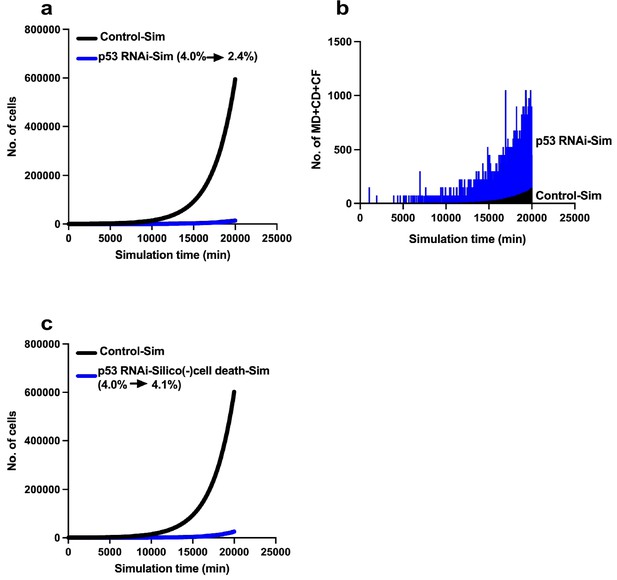
Limited expansion of p53 RNAi cells in a Control cell population.
We simulated the expansion of the p53 RNAi cell population (4% at the initial time point) in a Control cell population (96% at the initial time point) using Mixed culture mode with Operation data-Control and p53 RNAi for a simulation time of 20,000 min with 500 progenitors and repeating 10 simulations (total 5000 progenitors). (a) Simulation of 480 Control progenitors was carried out using Operation data-Control and 20 p53 RNAi progenitors with Operation data-p53 RNAi. The initial percentage of p53 RNAi cells was 4%, which was reduced to 2.4% at 20,000 min. (b) The sums of multipolar cell division, cell death, and cell fusion events (MD + CD + CF) are shown. (c) Simulation was performed using Operation data-p53 RNAi-Silico(-)cell death.
-
Figure 12—source data 1
Limiting expansion of p53 RNAi cells in a Control cell population.
Data used in Figure 12.
- https://cdn.elifesciences.org/articles/72498/elife-72498-fig12-data1-v3.xlsx
Cell-fate simulation of p53 RNAi cells in a Control cell population.
The p53 RNAi cells are indicated in blue. Other cells are indicated in gray. The animation video was created using data from the virtual cell-lineage database and Operation data-Control and p53 RNAi. After assigning the initial position of the cells, cell movement was created programmatically. When cell death occurred, virtual cells were split into small particles.
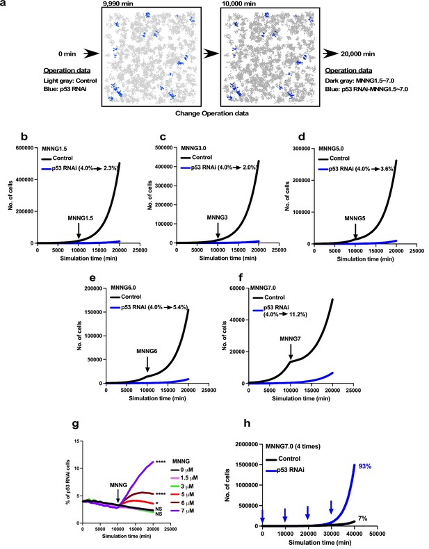
Expansion of p53 RNAi cells in a Control cell-dominant cell population subjected to virtual MNNG exposure.
We simulated the response of p53 RNAi cells in a Control cell-dominant cell population to MNNG exposure using Mixed culture- Switch mode. (a) The simulation was performed with 96% Control and 4% p53 RNAi cells, using Operation data-Control and p53 RNAi for 9900 min. The Operation data was then switched to, for example, MNNG7 and p53 RNAi-MNNG7 for virtual MNNG treatment, and the simulation was continued up to 20,000 min. In the animation (Figure 13—video 1), the pixel value of the image was reduced to indicate the virtual MNNG treatment. (b–f) In the simulation, Operation data corresponding to (b) 1.5, (c) 3, (d) 5, (e) 6, and (f) 7 µM MNNG were used to perform a virtual MNNG treatment. The numbers in the images indicate the percent of p53 RNAi cells at simulation times 0 and 20,000 min. (g) The percentages of p53 RNAi cells in the population are plotted. Statistical analysis (n = 10) was performed using data at simulation time 20,000 min by ordinary one-way ANOVA. NS, nonsignificant, *p<0.05, ****p<0.0001. (h) Based on the simulation data for 7 µM MNNG, percentage of p53 RNAi cells following repeated 7 µM MNNG exposure every 10,000 min (~7 days) was calculated. Arrows indicate the time that the virtual exposure was performed.
-
Figure 13—source data 1
Expansion of p53 RNAi cells in a Control cell population subjected to virtual MNNG exposure.
Data used in Figure 13.
- https://cdn.elifesciences.org/articles/72498/elife-72498-fig13-data1-v3.xlsx
Cell-fate simulation of p53 RNAi cells in a Control cell population subjected to virtual MNNG treatment.
The p53 RNAi cells are indicated in blue. Other cells indicated in gray. The animation video was created using data from the virtual cell-lineage database and Operation data-Control and p53si, and MNNG7 and p53 RNAi-MNNG7. The pixel value of the image was changed after virtual MNNG treatment at a simulation time of 10,000 min. After assigning the initial position of the cells, cell movement was created programmatically. When cell death occurred, virtual cells were split into small particles.
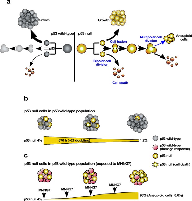
Role of the low levels of p53 in suppression of multipolar cell division, cell death, cell fusion, and damage response.
(a) Characteristics of Control and p53 RNAi cells. (b) The simulation of the fate of p53 RNAi cells in the Control cell population. (c) The simulation of the fate of p53 RNAi cells in the Control cell population, which were virtually exposed to 7 μM MNNG. The percentage of aneuploid cells is also shown.
Tables
| Reagent type (species) or resource | Designation | Source or reference | Identifiers | Additional information |
|---|---|---|---|---|
| Antibody | Mouse anti-p53 (DO-1, mouse monoclonal) | Invitrogen | AHO0152 | 1 µg/mL |
| Antibody | Horseradish peroxidase conjugated goat anti-mouse antibody (goat polyclonal) | Abcam | Ab205719 | 1:25,000 |
| Chemical compound, drug | N-methyl-N′-nitroso-N-nitrosoguanidine | Sigma-Aldrich | 129941 | |
| Cell line (human) | A549-luc-C8 | Xenogen Corporation | N/A | |
| Sequence- based reagent | p53 siRNA I | Cell Signaling Technology | 6231 | |
| Sequence- based reagent | Control siRNA | Cell Signaling Technology | 6568 | |
| Software, algorithm | MetaMorph (Quorum WaveFX, v7.8.12.0) | Quorum Technology | N/A | |
| Software, algorithm | ImageJ | Schneider et al., 2012 | https://imagej.nih.ggov/ij/ | |
| Software, algorithm | Computerized single-cell lineage tracking analysis system software | Rancourt, Sato, and Satoh | BioRxiv. doi: https://doi.org/10.1101/508705 | |
| Software, algorithm | Cell fate simulation algorithm | This paper | Results: ‘Cell-fate simulation algorithm’; Materials and methods: ‘Overall flow of cell-fate simulation algorithm’; Figure 7—source code 1 | |
| Other | Cell lineage data | This paper | Deposited in Dryad |


