Using positional information to provide context for biological image analysis with MorphoGraphX 2.0
- Max Planck Institute for Plant Breeding Research, Department of Comparative Development and Genetics, Germany
- John Innes Centre, Norwich Research Park, United Kingdom
- Institute of Imaging and Computer Vision, RWTH Aachen University, Germany
- IRBV, Department of Biological Sciences, University of Montreal, Canada
- Plant Developmental Biology, TUM School of Life Sciences, Technical University of Munich, Germany
- School of Life Sciences, University of Warwick, United Kingdom
Figures
Figure 1 with 1 supplement
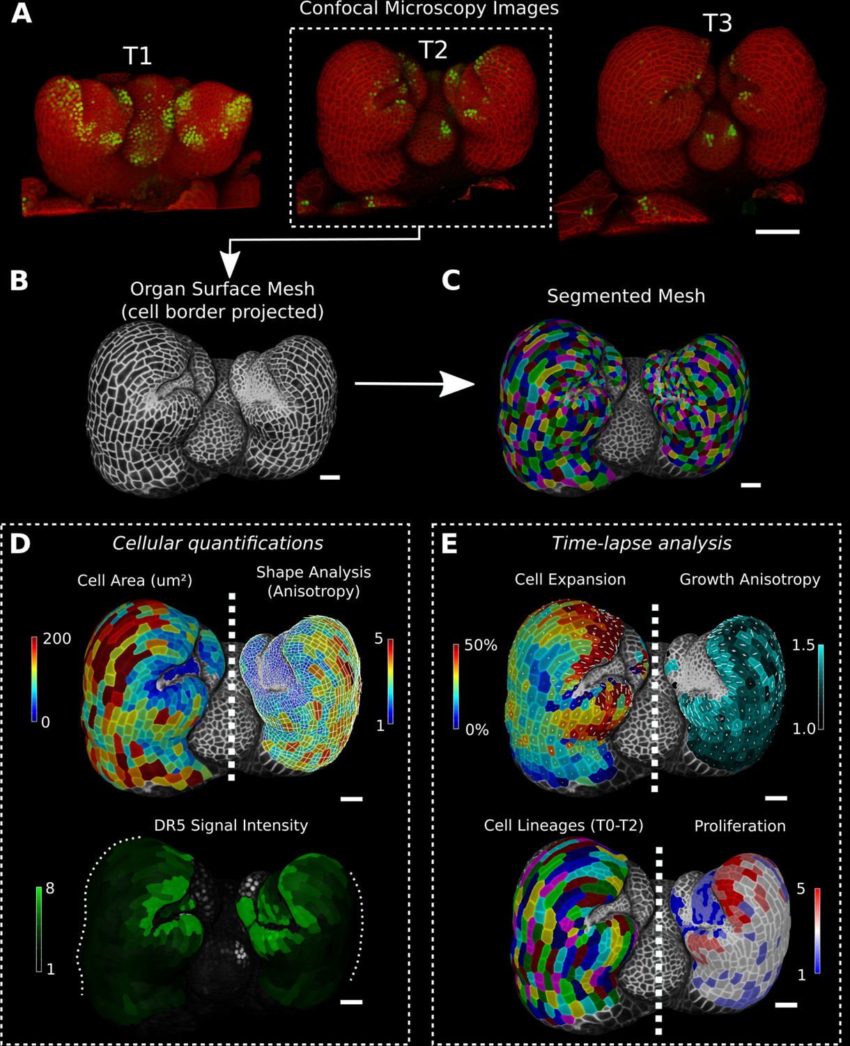
Cellular segmentation and basic quantifications supported by MorphoGraphX demonstrated by using a time-lapse series of an A. thaliana flower meristem.
(A) Multichannel confocal microscopy images with a cell wall signal (red) and DR5 marker signal (green). Shown are the last three time points (T1–T3) of a four-image series (T0–T3). (B, C) Extracted surface mesh of T2. Cell wall signal near the surface was projected onto the curved mesh to enable the creation of the cellular segmentation in (C). The segmented meshes provide the base for further analysis within MorphoGraphX as shown in (D) and (E). (D) Top: MorphoGraphX allows the quantification of cellular properties such as cell area and shape anisotropy (shown as heat maps). The white axes show the max and min axes of the cells. Bottom: heat map of the quantification of the DR5 marker signal (arbitrary units) projected onto the cell surface mesh. (E) When cell lineages are known, time-lapse data can be analyzed. Top: heat maps of cell area expansion and growth anisotropy (computed from T1 to T2). The white crosses inside the cells depict the principal directions of growth. Bottom: visualization of the cell lineages and heat map of cellular proliferation (number of daughter cells), computed from T0 to T2. Scale bars: (A) 50 μm; (B– E) 20 μm. See also user guide Chapters 1–15 and tutorial videos S1 and S2 videos S1 and S2available at https://doi.org/10.5061/dryad.m905qfv1r.
Figure 1—figure supplement 1
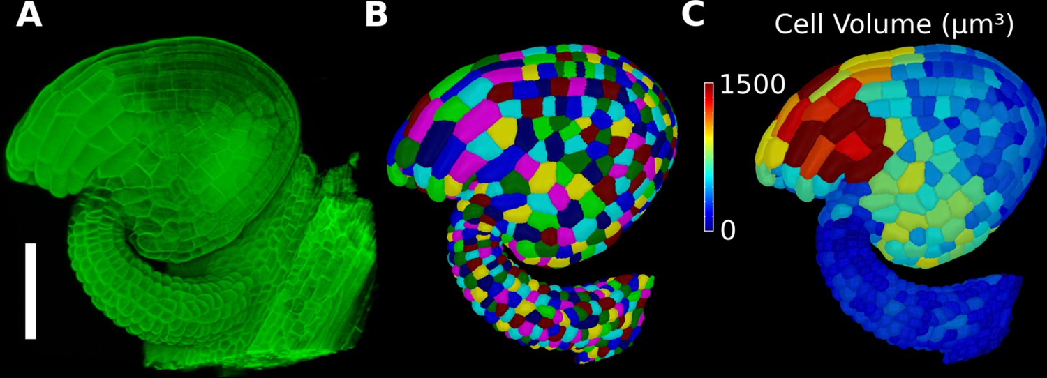
Basic 3D analysis using MorphoGraphX demonstrated using an Arabidopsis ovule.
(A) Confocal microscopy image with cell wall staining. (B) Segmented mesh with volumetric cells. (C) The segmented mesh allows cellular geometry to be quantified. Shown is a heat map of cell volumes. Scale bar: 50 μm. See also user guide Chapters 20–21 and tutorial video S6 available at https://doi.org/10.5061/dryad.m905qfv1r.
Figure 2 with 1 supplement
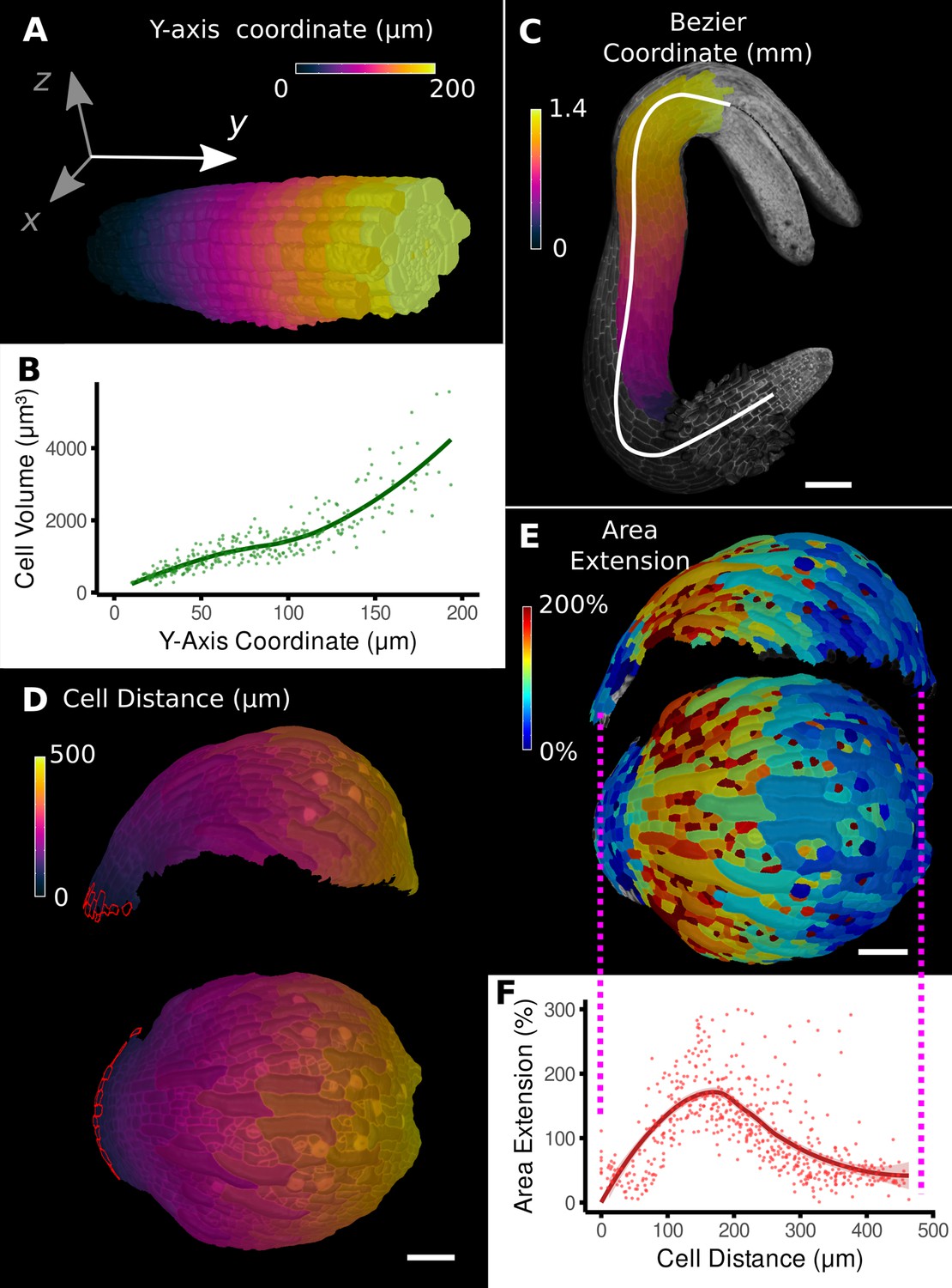
Methods to define positional information and their application to data analysis in plant organs.
(A) Y-axis aligned A. thaliana root. The cells are colored according to the y-coordinate of their centroid position. (B) Plot of cell volumes of epidermis cells of the root in (A) along the y-axis with a fitted trend line. (C) Seedling of A. thaliana with a surface segmentation of the epidermis. A manually defined Bezier curve (white) allows the assignment of accurate cell coordinates along a curved organ axis. (D) Side and top views of an A. thaliana sepal with a proximal-distal (PD) axis heat coloring. The cell coordinates were assigned by computing the distance to manually selected cells (outlined in red) at the organ base. This method allows organ coordinates to be assigned in highly curved tissues. (E) Side and top views of (D) with a heat map coloring based on cellular growth to the next time point. (F) Plot summarizing the growth data of (E) using the PD-axis coordinates from (D). See Figure 2—figure supplement 1 for the analysis of the complete time-lapse series. Scale bars: (A) 20 μm; (C) 100 μm; (D, E) 50 μm. See also user guide Chapter 23 ‘Organ-centric coordinate systems’ and tutorial video S3video S3 available at https://doi.org/10.5061/dryad.m905qfv1r.
Figure 2—figure supplement 1
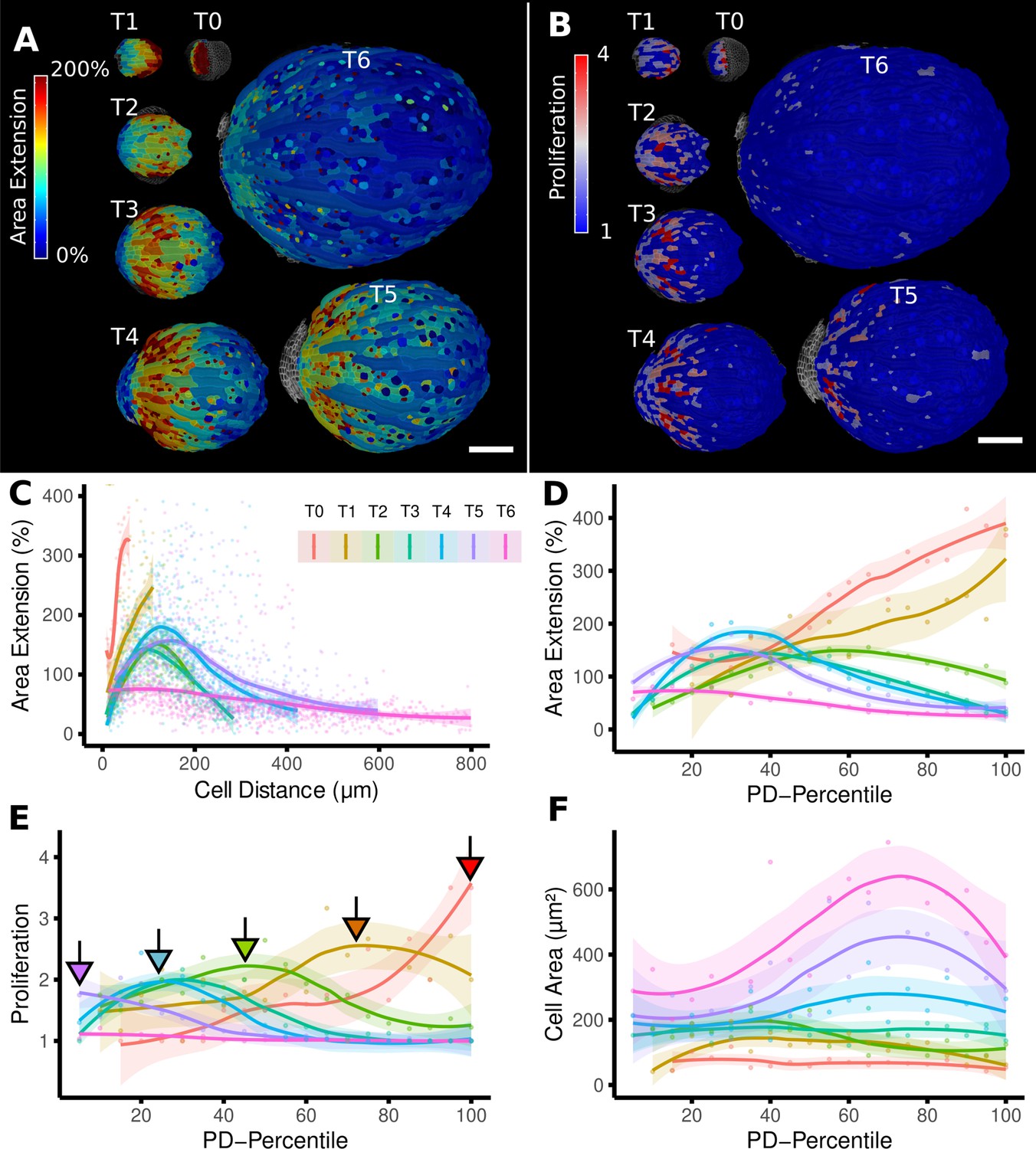
From cellular resolution heat maps to a global analysis of A. thaliana sepal development using organ-centric coordinates.
(A, B) Heat maps of cell area extension (A) and cell proliferation (B) for each time point (visualized on the earlier point). (C) Plot of the heat map data from (A) vs. the distance of cells to the base of the organ (see also Figure 2D). The distance of the maximum of the growth zone from the base or the organ is relatively constant. However, organ length increases about 10× between the first and last time points, making a comparison of the different curves difficult. (D–F) When plotting the same data with normalized cell distance values averaged using 20 bins along the proximal-distal axis, it becomes more apparent that the growth zone moves from the proximal to the distal regions over the course of development (D). The trend of lower and more proximal maxima (highlighted with arrows) is even clearer when proliferation is plotted in the same way (E). (F) Cell area data plotted as in (D) and (E). Average cell areas increase mainly at the distal end during later time points. Scale bars: (A, B) 100 μm.
Figure 3
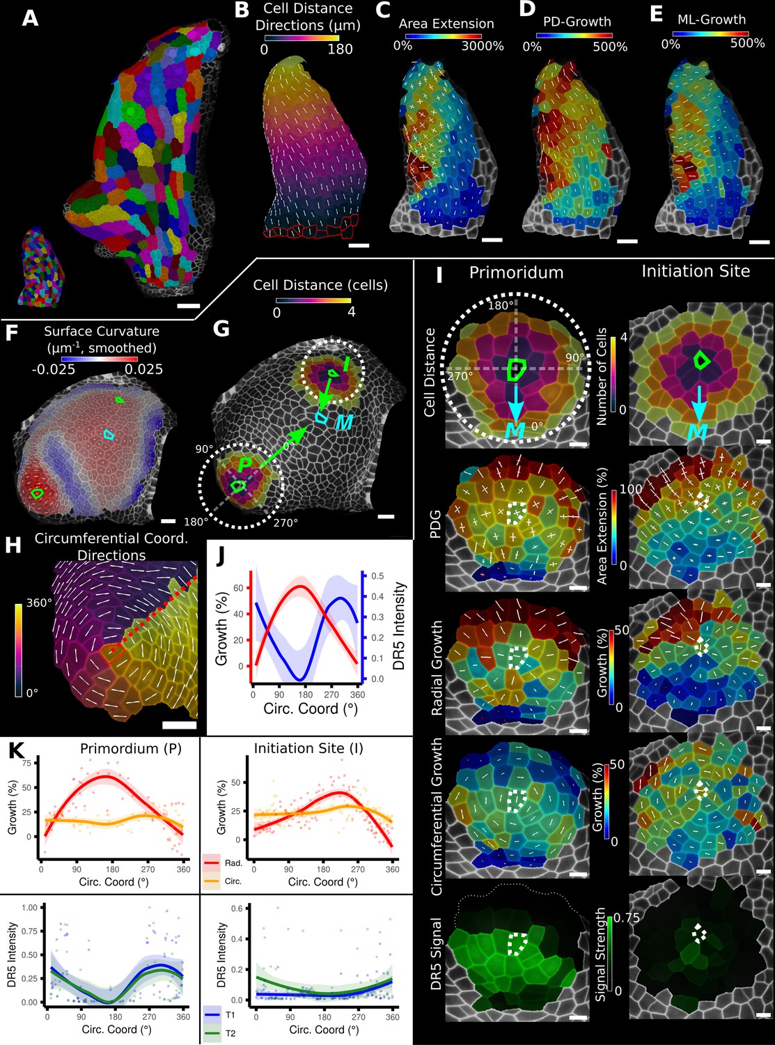
Examples of data analyses using organ coordinate directions.
(A–E) Quantification of cellular growth along organ axes in a young A. thaliana leaf. (A) Segmented meshes of the leaf primordium at 3 and 6 days after initiation shown with cell labels and lineages of the earlier time point (3 days). (B) Earlier time point of (A) with proximal-distal (PD) axis coordinates (heat map) and directions (white lines) computed from selected cells at the leaf base. (C) Area extension (heat map) and principal directions of growth (PDGs, white lines) between the time points of (A). PDG axes are computed per cell and can point in different directions. (D, E) Computation of the growth component of (C) that is directed along the PD and the orthogonal medial-lateral (ML) axis. (F–K) Quantification of locally directed growth in leaf primordium and initiation site of a tomato meristem. (F) Smoothed heat map of cell curvature. Local maxima in this heat map (green and cyan cells) were selected as meristem center (M), primordium center (P), and initiation site (I) as shown in (G). (H) To analyze the data, we defined circumferential coordinate systems with their axes directions (white lines) around the primordium and initiation center (not shown), and aligned them towards the meristem center. (I) Heat maps of cell distance, area extension, radial and circumferential growth, and normalized DR5 signal intensity of the aligned primordium and initiation site. (J) Plotting the data of (I) reveals a negative correlation of the DR5 signal intensity and radial growth around the developing primordium. (K) Detailed plots of radial (red) and circumferential growth (orange) as well as the normalized DR5 signal intensity of the primordium and initiation site. Scale bars: (A) 50 μm; (B–H) 20 μm; (I) 10 μm. See also user guide Chapters 16 ‘Custom axis directions,’ 23 ‘Organ-centric coordinate systems,’ and tutorial video S3 available at https://doi.org/10.5061/dryad.m905qfv1r.
Figure 4 with 1 supplement
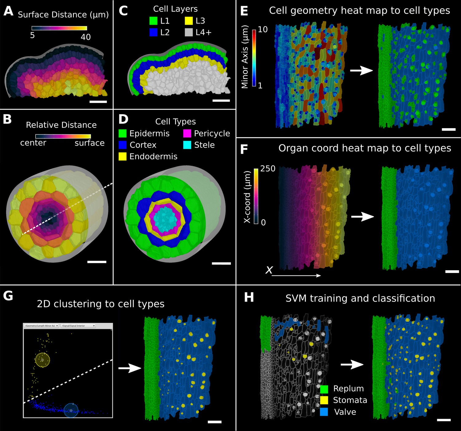
Methods to create organ coordinates for 3D meshes and label different cell types.
(A–D) Organ coordinates and cell types for volumetric meshes. (A) Heat map of the surface distance for cell centroids in an A. thaliana shoot apical meristem. (B) For volumetric tissues, often a single direction is not enough to capture the geometry of the organ. Different methods can be combined such as a Bezier curve (white dashed line) with a surface mesh (gray) to create a heat map of the relative radial distance of cells in the A. thaliana root. (C, D) Organ coordinates can be used to assign cell-type labels as demonstrated in the 3D Cell Atlas plug-in for meristem and root. See also Figure 4—figure supplement 1. (E–H) Different methods to create cell-type labelings. (E) A. thaliana gynoecium (fruit epidermis) surface segmentation with a heat map of the length of the minor cell axis as obtained from a principal component analysis (PCA) on the cells’ triangles. The heat values can be thresholded to assign two cell types. (F) The same principle can be used on organ coordinates that results in a clean separation of replum (green) and valve tissue (blue). (G) We generalized the 2D clustering approach of 3D Cell Atlas (see Figure 4—figure supplement 1) so that it can be used for any measure pair and on subset selections of cells. Shown is a 2D plot of the minor axis length (x-coord) and cell signal intensity (y-coord) on the valve tissue in (F). Manually assigning clusters can separate the stomata, which are typically smaller with higher signal values (yellow) and the remaining valve cells (blue) efficiently. See also Figure 4—figure supplement 1 for 2D plots of all cells. (H) The support vector machine (SVM) classification is able to separate the three shown cell types in a higher dimensional space by using a variety of different measures and a relatively small training set. Scale bars: (A–D) 20 μm; (E–H) 50 μm. See also user guide Chapter 24 ‘Cell atlas and cell type classification’ and tutorial videos S3 and S4 available at https://doi.org/10.5061/dryad.m905qfv1r.
Figure 4—figure supplement 1

Cell-type labeling methods and their use in the data analysis.
(A–C) Methods supported by the 3D Cell Atlas add-on demonstrated on a A. thaliana root (Montenegro-Johnson et al., 2015). (A) Longitudinal cross section with a heat map of circumferential cell size. The white dashed line is the manually defined central axis. (B) The 2D heat plot of radial distance (heat map: in Figure 4B) and circumferential cell size (heat map in A) reveals a distinct clustering and can be used directly to assign the different cell types (dashed ellipses). (C) Final result of the cell-type assignment. (D) The 3D Cell Atlas meristem (Montenegro-Johnson et al., 2019) allows the assignment of cell layers (as also seen in Figure 4C) and types in the meristem. (E–G) Cell-type-specific data analysis on the example of the A. thaliana gynoecium (Figure 4E–H). (E) Violin plot of the rectangularity of different cell types. Valve tissue cells are less rectangular and have higher variance compared to replum cells and stomata. (F, G) 2D scatter plots with fitting ellipses. Choosing different measures as x- or y-axis allows the separation of different cell types as demonstrated in Figure 4G. Scale bars: (A, C, D) 20 μm.
Figure 5
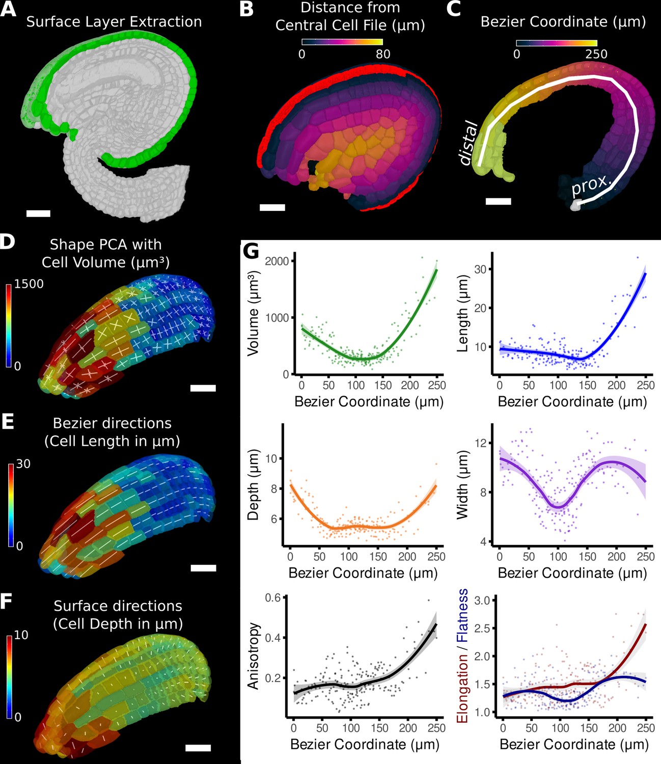
Quantification of volumetric cell sizes along organ axes in the outer layer of the outer integument of an A. thaliana ovule.
(A) Extraction of cell layer of interest (colored in green) using an organ surface mesh. (B) Selection of the central cell file (in red) with cell distance heat map to exclude lateral cells (heat values >40 µm). (C) The centroids of the selected cells from (B) were used to specify a Bezier curve defining the highly curved organ axis from the proximal to the distal side. Heat coloring of the cells according to their coordinate along the Bezier. (D–F) Analysis of the cellular geometry in 3D. (D) Heat map of cell volume and the tensor of the three principal cell axes obtained from a principal component analysis on the segmented stack. (E) Bezier directions and associated cell length. (F) Directions perpendicular to the surface and associated cell depth. (G) Plots of the various cellular parameters relative to the Bezier coordinate. A few small cells at the distal tip of the integuments were removed from the analysis. Scale bars: 20 μm. See also user guide Chapters 21–24 and tutorial video S3 available at https://doi.org/10.5061/dryad.m905qfv1r.
Figure 6 with 1 supplement
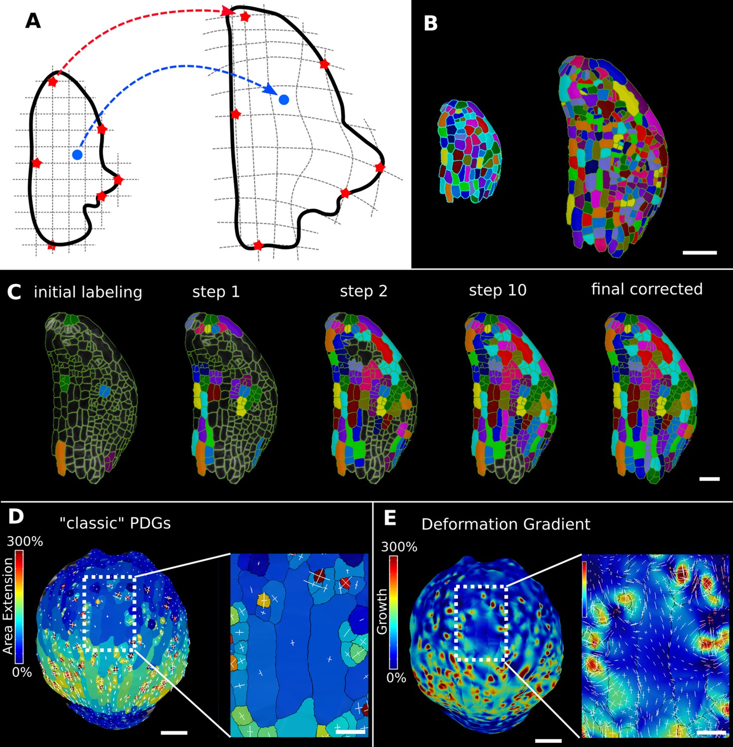
Deformation functions in MorphoGraphX.
(A) Deformation functions allow a direct mapping of arbitrary points (blue) between two meshes. They require the definition of common landmarks (red stars). (B, C) Semi-automatic parent labeling using deformation functions. (B) Two consecutive time points of an A. thaliana leaf primordium segmented into cells. (C) The automatic parent labeling function requires the definition of a few manually labeled cells as initial landmarks. From this sparse correspondence, a mapping between the meshes can be created and new cell associations between the two meshes are added and checked for plausibility. With more cells found, the mapping between the meshes is improved for the next iteration. (D, E) Comparison of the classic principal directions of growth (PDGs) in (D) with the gradient of a deformation function computed using the cell junctions from a complete cell lineage in (E) on an A. thaliana sepal. The classic PDGs compute a deformation for each cell individually and are shown with a heat map of areal extension for each cell. In contrast, the deformation function is a continuous function on the entire mesh. Here, heat values are derived by multiplying the amount of max and min growth. Using the deformation function gradient subcellular growth patterns that were previously hidden are revealed, such as differential growth within a single giant cell. Scale bars: (B, D, E) 50 μm; (C and zoomed regions in D and E) 20 μm. See also user guide Chapter 17 ‘Mesh deformation and growth animation’ and tutorial videos S1 and S2 available at https://doi.org/10.5061/dryad.m905qfv1r.
Figure 6—figure supplement 1
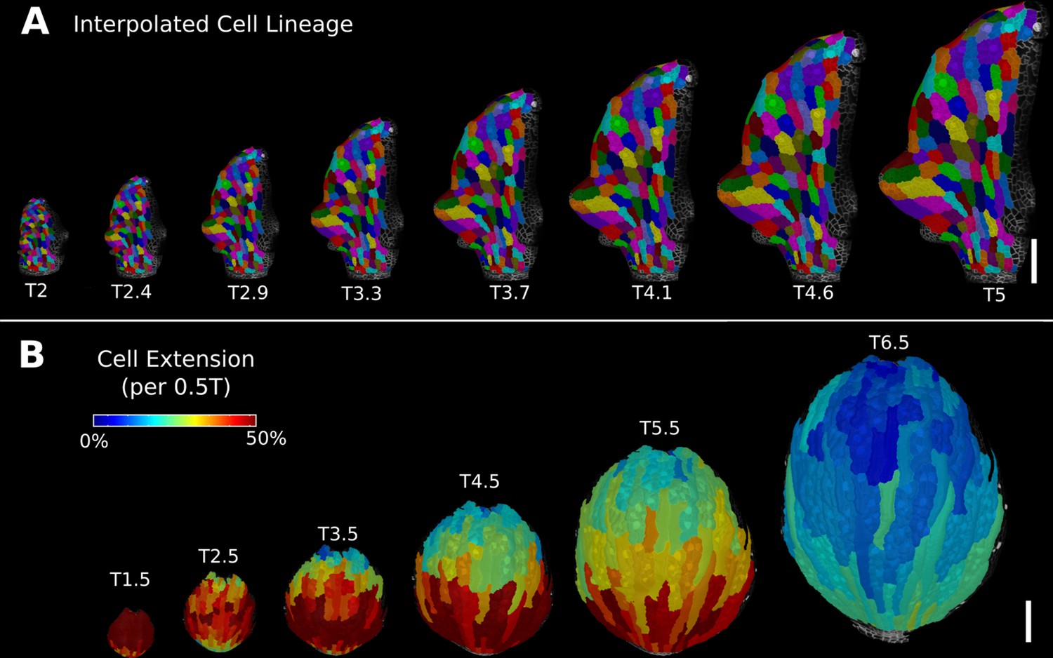
Deformation functions allow the interpolation of intermediate steps that can be turned into a continuous sequence or animation.
(A) Animation of the early leaf development of A. thaliana created from T2 and T5 of Figure 5, shown with the lineages of T2. (B) Intermediate stages of the animation of the sepal growth of A. thaliana. For the actual time points, see Figure 2—figure supplement 1. Scale bars: 100 μm. See also user guide Chapter 17 ‘Mesh deformation and growth animation’” and tutorial video S5 available at https://doi.org/10.5061/dryad.m905qfv1r.
Figure 7 with 1 supplement

Time-lapse analysis and visualization of 3D meshes.
(A) Cross section of the confocal stack of the first time point of a live imaged A. thaliana root. (B, C) The 3D segmentations of two time points imaged 6 hr apart. Shown are the cell lineages that were generated using the semi-automatic procedure following a manual correction. (D) Exploded view of the second time point with cells separated by cell types (see also Figure 4D). Cells are heat colored by their volume increase between the two time points. (E–H) Quantification of cellular growth along different directions within the organ. (E) Plot of the heat map data of (D). The cellular data was binned based on the distance of cells from the quiescent center (QC). Shown are mean values and standard deviations per bin. (F–H) Similarly binned data plots of the change in cell length (F), width (G), and depth (H). It can be seen that the majority of growth results from an increase in cell length. See Figure 7—figure supplement 1 for a detailed analysis of the cells in the endodermis. (I) Different ways to visualize 3D growth demonstrated using a single cortex cell: principal directions of growth (PDGs) averaged over the entire cell volume (left), PDGs averaged over the cell walls projected onto the walls (top right), and subcellular vertex-level PDGs projected onto the cell walls (bottom right). Scale bars: (A–D) 20 μm; (I) 5 μm. See also user guide Chapter 21 ‘Mesh 3D analysis and quantification’ and tutorial videos S6 and S7 available at https://doi.org/10.5061/dryad.m905qfv1r.
Figure 7—figure supplement 1
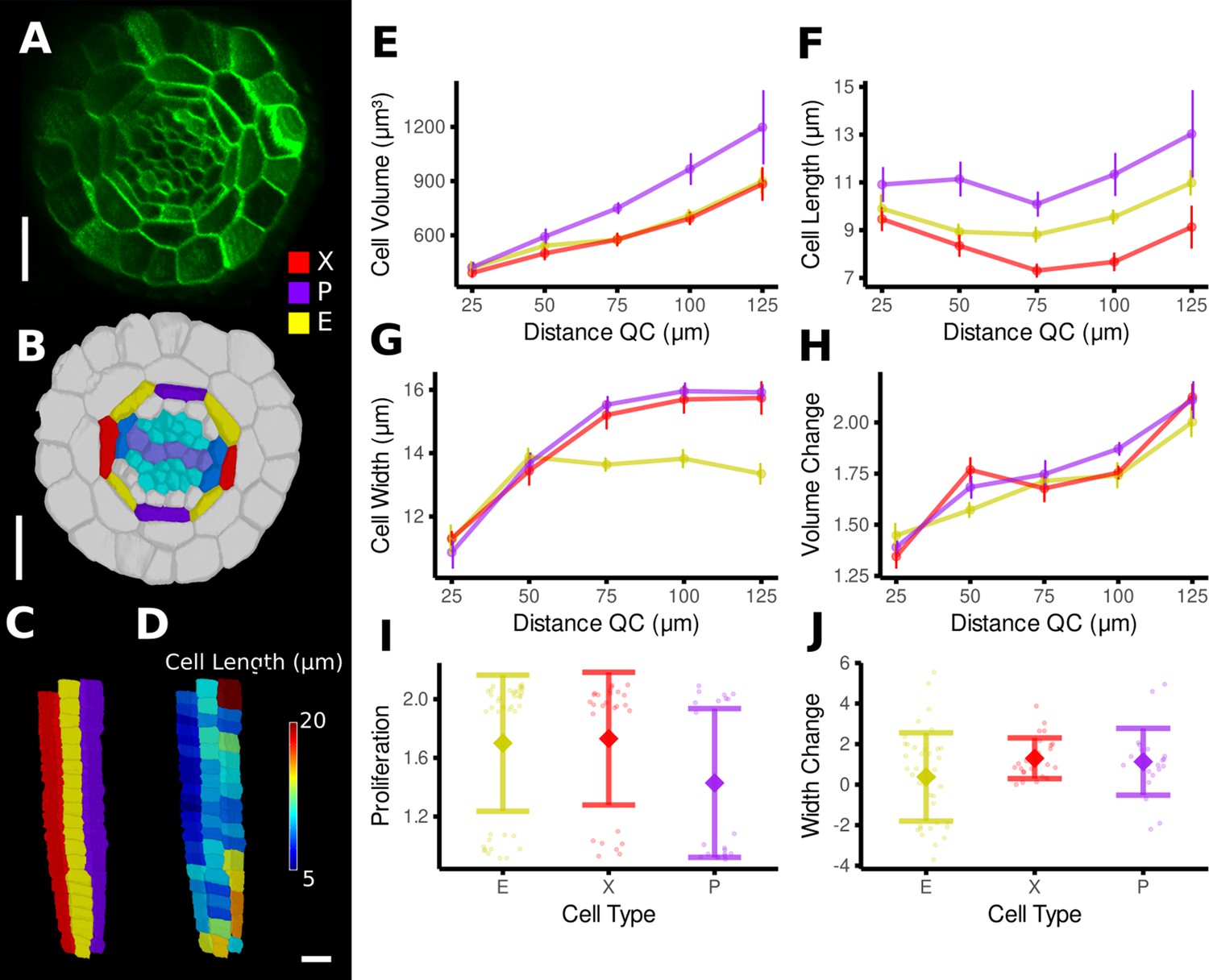
Time-lapse analysis of cellular geometry in the A. thaliana root endodermis.
(A) Cross section of the confocal image of time point 1. (B) Segmentation with extended cell-type labeling in the endodermis. The root cell-type labeling of Figure 4D was extended by identifying the xylem cells (light purple) in the stele (cyan), their adjacent pericycle cells (blue), and assigned the endodermis cells neighboring those pericycle cells as xylem file cells (X, red). Then the endodermis cells at right angles to the xylem files were assigned phloem file (P, purple) and the remaining other endodermis cells (E, yellow). (C) Side view of one cell file of each cell type. As the cell types do not change along the cell file, it was possible to automatically assign the cell files based on their circumferential coordinate. (D) Cell files of (C) with a heat map of cell length indicating smaller cells in the xylem pole. (E–J) Quantifications of cell geometry and development in the endodermis cell types. Cellular data was binned according to their distance from the quiescent center (QC) (E–H). Shown are mean values and standard deviations per bin (E–H) or cell type (I, J). Phloem file cells showed a larger volume (E), which was caused by a greater cell length (F), an observation that has been made before by Andersen et al., 2018. In contrast, xylem file and other endodermis cells were smaller in volume due to different reasons: while xylem file cells were the shortest (E), rest endodermis cells showed a lower cell width with increasing distance from the QC (G). The time-lapse analysis confirmed above observations: while volume change was similar across the cell types (H), phloem file cells showed a lower proliferation rate (I), whereas rest endodermis cells showed the smallest extension of cell width (J). Scale bars: (A, B) 20 μm; (C, D) 50 μm.
Figure 8 with 2 supplements
Advanced data analysis and visualization tools.
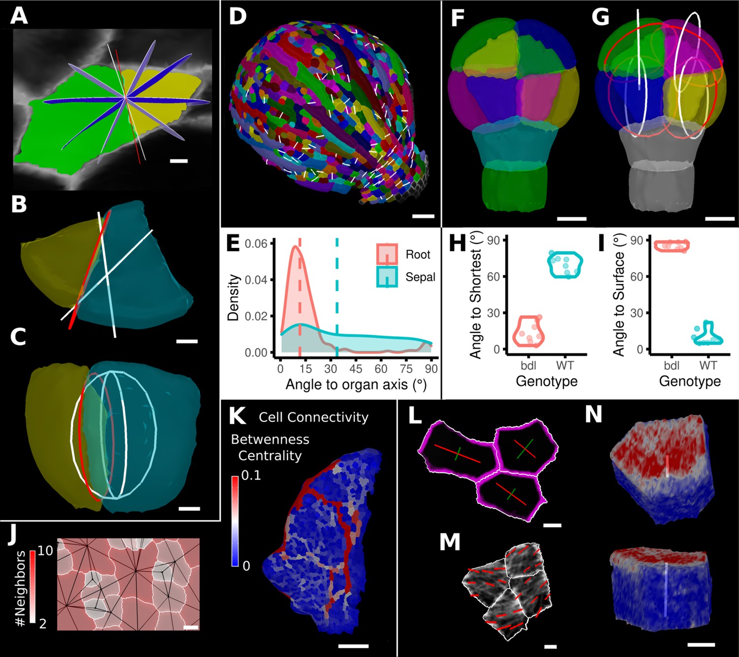
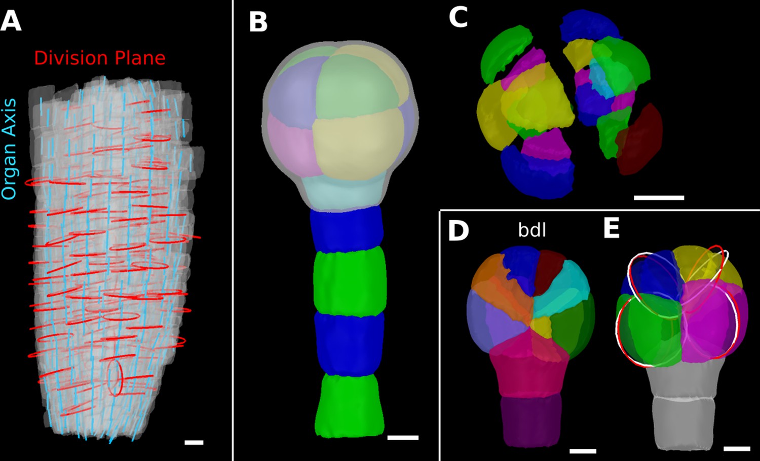
(A) Division analysis of a cell from a surface segmentation of an A. thaliana sepal. A planar approximation of the actual plane is shown in red and other potential division planes in white/blue. The actual wall is very close to the globally shortest plane. (B, C) Top and side views of a recently divided 3D segmented cell. The daughter cells are colored yellow and cyan. The red circle depicts the flat approximation plane of the actual division wall. The two white rings depict the two smallest area division planes found by simulating divisions through the cell centroid of the mother cell (i.e., the combined daughter cells). (D) Visualization of the actual planes (white lines) between cells that divided into two daughter cells in the A. thaliana sepal. (E) Density distribution and median (dashed line) of the angle between the division plane and the primary organ axis in sepal (see D) and root (see Figure 8—figure supplement 1A). The division in sepals is less aligned with the organ axis. (F) Half of an A. thaliana wildtype embryo in the 16-cell stage. This view shows that the divisions leading to this stage are precisely regulated to form two distinct layers in the embryo. (G) A visualization of the actual planes (red circles) and the shortest planes (white circles) in the wild type. Cells are colored according to the label of the mother cells. (H, I) Violin plots of quantifications of the planes show that the wild type does not follow the shortest wall rule unlike the auxin-insensitive-inducible bdl line RPS5A>>bdl. The bdl divisions are almost orthogonal to the organ surface (see Figure 8—figure supplement 1B, D, E), whereas the wild type divides parallel to the surface. Consequently, the bdl fails to form a distinct inner layer. (J, K) Cellular connectivity network analysis. (J) Cell connectivity network analysis on a young A. thaliana leaf. Cells are heat colored based on the number of neighbors, edges in the cell connectivity graph are shown in black. (K) Heat map of betweenness centrality. The betweenness reveals pathways that might be of importance for information flow, potentially via the transport of auxin. (L–N) Cell-based signal analysis. (L) Analysis of cell polarization on a surface mesh. (M) Microtubule signal analysis on a surface mesh. (N) Top and side views of a cell polarization analysis on a volumetric mesh (root epidermis PIN2, see Figure 8—figure supplement 2A–D for details). Scale bars: (A, B, C, L, M) 2 μm; (D) 50 μm; (F, G, J, N) 5 μm; (K) 100 μm. See also user guide Chapter 25 ‘Cell division analysis.’, Chapter 18 'Quantifying signal orientation', and Chapter 21.7 'Signal orientation for 3D meshes'.
Figure 8—figure supplement 1
Details of the cell division analysis examples from Figure 8.
(A) Second time point of an A. thaliana root (see Figure 7C) that was used for the division plane analysis in Figure 8E. Cells are shown semi-transparently (gray) with their longitudinal organ axis (cyan) obtained from the analysis using 3D Cell Atlas in Figure 4B. Planar approximations of the division planes between cells that divided between the two time points are shown as red circles. Consistent with the quantitative analysis in Figure 8E, most planes are aligned with the organ axis. (B, C) A. thaliana wildtype embryo at the 16-cell stage segmented into volumetric cells shown with an organ surface mesh (gray, semi-transparent, B) and shown in an exploded view (C) to enable the visualization and access of inner layers. (D, E) Corresponding panels to Figure 8F and G for bdl embryo. Scale bars: (A–C) 10 μm; (D, E) 5 μm.
Figure 8—figure supplement 2

Example analyses of cell polarity and microtubule signals of the data shown in Figure 8M and N.
(A–D) Quantification of PIN2 polarity in volumetric cells of an A. thaliana root. (A, B) Heat map of PIN2 concentration on epidermis and cortex. Green lines depict directionality and strength of the PIN2 concentration. (C, D) Violin plots of the orientation data for division planes and PIN2 polarity for epidermis and cortex cells. Epidermis cells show considerably stronger polarity (D) and are more aligned with the (longitudinal) organ axis (C). (E, F) Microtubule analysis on a shoot apical meristem (SAM) of A. thaliana. (E) The cells on the SAM were binned according to their distance to the SAM center. Cells are heat colored according to their bin. Yellow lines show the direction and strength of the microtubule orientation. (F) Boxplot of the angular difference between microtubule orientation and the circumferential direction around the center of the SAM (similar to Figure 5H). Scale bars: (A, B) 20 μm; (E) 10 μm. See also user guide Chapter 18 ‘Quantifying signal orientation.’ and Chapter 21.7 'Signal orientation for 3D meshes'.
Videos
Video 1
Creation of a simple organ-centric coordinate system and its application on cellular data.
Starting with two time points of an Arabidopsis sepal that have been lineage traced, the principal directions of growth are computed. Next, cells at the base of the sepal are selected to create a distance field that is used as a simple coordinate system. The growth (areal extension) can then be computed along the directions defined along the organ-centric coordinate system. The organ coordinates can also be exported and used to plot different kinds of cellular data.
Video 2
Cell-type classification using support vector machines (SVMs).
A selection of measures is calculated on a segmented mesh from an Arabidopsis gynoecium. A sampling of cells are then are labeled by hand and used as training data. The cell type for the rest of the cells is then predicted automatically.
Video 3
Semi-automatic cell lineage tracking.
A few cells from two time points from a time lapse of Marchantia are matched by hand. The other cells can then be determined automatically. Trouble spots can be overcome by selecting a few more cells by hand and continuing the process.
Video 4
Animating time-lapse data with deformation functions.
A time lapse of Marchantia is used to demonstrate how deformation functions can be used to animate growth. Cells are colored by areal growth rate.
Video 5
Creating an animation.
Key frames are saved and used to provide steps for an animation that can then be played back.
Video 6
Convolutional neural network (CNN) cell wall prediction and segmentation.
Using an Arabidopsis flower meristem, a CNN is first used to improve the cell wall signal. The meristem is then segmented into cells, and a 3D mesh created.
Video 7
Calling R from MorphoGraphX.
A time lapse of an Arabidopsis leaf is used to demonstrate how to create heat map data for analysis and plotting in R.
Tables
Table 1
Measures for cells segmented on surface projections (2.5D).
| Measure | Unit | Description |
|---|---|---|
| Geometry | ||
| Area | µm2 | Area of the cell (sum of its triangle area) |
| Aspect ratio | - | Ratio of length major axis and length minor axis (see below) |
| Average radius | µm | Average distance from the center of gravity of a cell to its border |
| Junction distance | µm | Max or min distance between neighboring junctions of a cell |
| Length major axis | µm | Length of the major axis of the 2D shape analysis (computes a PCA on the triangle positions weighted by their area) |
| Length minor axis | µm | Length of the minor axis of the 2D shape analysis (computes a PCA on the triangle positions weighted by their area) |
| Maximum radius | µm | Maximum distance from the cell center to its border |
| Minimum radius | µm | Minimum distance from the cell center to its border |
| Perimeter | µm | Sum of the length of the border segments of a cell |
| Lobeyness | ||
| Circularity | - | Perimeter^2/(4*PI*Area) |
| Lobeyness | - | Ratio of cell perimeter to convex hull perimeter (1 for convex shapes) |
| Rectangularity | - | Ratio of cell area to the area of the smallest rectangle that can contain the cell (1 for rectangular shapes, lower values for irregular shapes) |
| Solidarity | - | Ratio of the convex hull area to the cell area (1 for convex shapes, higher values for complicated shapes) |
| Visibility pavement | - | 1-(visibility stomata) (see below) |
| Visibility stomata | - | Estimate of visibility in the cell 1 for convex shapes, decreases with the complexity of the contour |
| Location | ||
| Bezier coord | µm | Associated Bezier coordinate of a cell Requires a Bezier grid |
| Bezier line coord | µm | Associated Bezier coordinate of a cell Requires a Bezier curve |
| Cell coordinate | µm | Cartesian coordinate of a cell |
| Cell distance | µm/cells | Distance to the nearest selected cell (finds the shortest path to a selected cell through the cell connectivity graph, edge weights: Euclidean, cell number or 1/wall area) |
| Distance to Bezier | µm | Euclidean distance to the Bezier curve or grid |
| Distance to mesh | µm | Euclidean distance to the nearest vertex in the other mesh |
| Major axis theta | ° | Angle between the long axis of the cell and a reference direction |
| Polar coord | °/µm | Polar coordinate around a specified Cartesian axis |
| Network | ||
| Neighbors | Count | Number of neighbors of a cell |
| Betweenness centrality | - | Computes the betweenness centrality of the cell connectivity graph Edges can be weighted by the length of the shared wall between neighboring cells |
| Betweenness current flow | - | Computes the betweenness current flow of the cell connectivity graph Edges can be weighted by the length of the shared wall between neighboring cells |
| Signal | ||
| Signal border | Average amount of border signal in a cell | |
| Signal interior | Average amount of interior signal in a cell | |
| Signal parameters | Advanced and general process that allows the setting of parameters to compute different kinds of signal quantifications | |
| Signal total | Average amount of total (=border + interior) signal in a cell | |
| Other measure processes | ||
| Mesh/lineage tracking/heat map proliferation | Cells | Proliferation |
| Mesh/cell axis/custom/custom direction angle | ° | Angle between a cell axis and a custom axis |
| Mesh/division analysis/compute division plane angles | ° | Angle between division planes and/or cell axes |
-
PCA: principal component analysis.
Table 2
Measures for meshes with volumetric (3D) cells.
| Measure | Unit | Description |
|---|---|---|
| Cell atlas | ||
| Cell length (circumferential, radial, longitudinal) | µm | Cell length as determined by 3D Cell Atlas root (shoot rays from the cell center to the side walls to measure cell size along organ-centric directions) |
| Coord (circumferential, radial, longitudinal) | 3D organ coordinates as determined by 3D Cell Atlas root | |
| Geometry | ||
| Cell length (custom, X, Y, Z) | µm | Cell length along the specified direction (cell size is measured as in 3D Cell Atlas root [see above]) |
| Cell wall area | µm2 | Total area of the cell wall |
| Cell volume | µm3 | Volume of the cell |
| Outside wall area | µm2 | Cell wall area that is not shared with another neighboring cell |
| Outside wall area ratio | % | Proportion of cell wall area that is not shared with a neighbor cell |
| Location | ||
| Bezier coord | µm | Associated Bezier coordinate of a cell Requires a Bezier curve or grid |
| Cell coordinate | µm | Cartesian coordinate of a cell |
| Cell distance | µm/cells | Distance to the nearest selected cell (finds the shortest path to a selected cell through the cell connectivity graph, edge weights: Euclidean, cell number or 1/wall area) |
| Distance to Bezier | µm | Euclidean distance to the Bezier curve or grid |
| Mesh distance | µm | Euclidean distance to the nearest vertex in the other mesh |
| Network | ||
| Neighbors | Count | Number of neighbors of a cell |
| Betweenness centrality | - | Computes the betweenness centrality of the cell connectivity graph Edges can be weighted by the length of the shared wall between neighboring cells |
| Betweenness current flow | - | Computes the betweenness current flow of the cell connectivity graph Edges can be weighted by the length of the shared wall between neighboring cells |
Table 3
MorphoGraphX workflows.
| Workflow | Description | Used in figure | User guide chapter |
|---|---|---|---|
| MorphoGraphX legacy workflows | Processes and pipelines introduced in MorphoGraphX 1.0 (Barbier de Reuille et al., 2015) | ||
| Surface segmentation | Creating a surface mesh, projecting epidermal signal and segmentation | Figure 1A–C | The chapters at the beginning of the user guide deal with these basic topics: from chapter 1 ‘Introduction’ to 12 ‘Attribute maps & data export’ |
| 3D segmentation | Creating volumetric segmentation using ITK watershed | Figure 1—figure supplement 1A and B | 20 ‘3D segmentation’ |
| Parent labeling | Cell lineage tracing between two subsequent segmented time points of the same sample | Figure 1D and E | 13 ‘Lineage tracking’ |
| Cell geometry heat maps | Creating heat map of cellular data | Figure 1D, Figure 1—figure supplement 1C | 10 ‘Cell geometry quantification’ |
| Time-lapse heat maps | Creating heat maps using two parent labeled time points | Figure 1E | 14 ‘Comparing data from two time points’ |
| Growth directions | Computing growth directions using time-lapse data | Figure 1E | 15 ‘Principal directions of growth (PDGs)’ |
| MorphoGraphX 2 workflows | New processes and pipelines introduced in this article | ||
| Different methods of creating organ coordinates | Using world coordinates (X, Y, Z) | Figure 2A | 23.3 ‘Further types of organ coordinates’ |
| Using polar coordinates | Figure 3G–I | 23.3 ‘Further types of organ coordinates’ | |
| Using Bezier line or grid | Figure 2C | 23.2 ‘Bezier line and grid’ | |
| Using cell distance heat maps | Figure 2D | 23.1 ‘The cell distance measure’ | |
| Using a separate organ surface mesh | Figure 4A | 23.3 'Further types of organ coordinates' | |
| Different methods of creating cell-type labelings | Using heat maps or organ coordinates | Figure 4E and F | 24.4 ‘Cell type classification using a single heat map’ |
| Using 2D clustering | Figure 4G | 24.5 ‘Cell type classification using two measures’ | |
| Using support vector machines (SVMs) | Figure 4H | 24.6 ‘Cell type classification using SVMs’ | |
| Organ directions | Deriving directions from coordinates or Bezier curves | Figure 3B and H | 16 ‘Custom axis directions’ and 21.6 ‘Custom directions for 3D meshes’ |
| Combining directions | Combining different kind of organ coordinates or directions | Figure 4B, Figure 5D–F | 24.1 ‘Cell Atlas root” and 21.6 ‘Custom directions for 3D meshes’ |
| Semi-automatic parent labeling | For lineage tracing | Figure 6A–C | 17.2 ‘Semi-automatic parent labeling’ |
| Morphing animations | Figure 6—figure supplement 1A and B | 17.4 ‘Morphing animations’ | |
| 3D growth analysis | Figure 7D–I | 21.3 ‘Change maps 3D’ and 21.4 ‘PDGs 3D’ | |
| Division analysis | Analyzing cell divisions | Figure 8A–I, Figure 8—figure supplement 1A and E | 25 ‘Division analysis’ |
| Cell connectivity analysis | Analyzing cellular connectivity networks | Figure 8J and K | - |
| 3D visualization | Exploded views | Figure 8—figure supplement 1C | 21.5 ‘3D visualization options’ |
| Signal quantification | Quantifying signal amount and direction | Figure 8L–N, Figure 8—figure supplement 2A–F | 18 ‘Quantifying signal orientation’ and 21.7 ‘Signal orientation for 3D meshes’ |
Additional files
Download links
A two-part list of links to download the article, or parts of the article, in various formats.
Downloads (link to download the article as PDF)
Open citations (links to open the citations from this article in various online reference manager services)
Cite this article (links to download the citations from this article in formats compatible with various reference manager tools)
Using positional information to provide context for biological image analysis with MorphoGraphX 2.0
eLife 11:e72601.
https://doi.org/10.7554/eLife.72601


