Nanofluidic chips for cryo-EM structure determination from picoliter sample volumes
- Department of Bionanoscience, Kavli Institute of Nanoscience, Delft University of Technology, Netherlands
- SmartTip B.V., Netherlands
- Structural and Computational Biology Unit, European Molecular Biology Laboratory (EMBL), Germany
Figures
Figure 1 with 2 supplements

A nanofluidic sample support for cryo-EM.
(a) Schematic representation of the MEMS-based cryoChip. The 2 × 2 mm chip base features two microcantilevers for sample filling and air escape. The cantilevers are connected to microchannels leading to a free-standing observation membrane located within an aperture at the chip center (middle inset). A multifurcation connects the microchannels (blue) to an array of five parallel nanochannels (yellow) of approximately 700 nm width and 100 nm height (rightmost inset). The top membrane is smoothly sagging, while the bottom membrane is flat. (b) False-colour scanning electron microscopy (SEM) image of the observation membrane. (c) False-colour SEM image of a single nanochannel with FIB-milled rectangular opening across the observation membrane (d) Ellipsometric determination of SiNx membrane thickness after deposition and etching steps. (e) Relative thickness map of an ice-filled nanochannel from zero-loss imaging. WET = water-equivalent thickness, IT = ice thickness. The thickness profile correlates with a 2D slice of a tomogram acquired of the same area (bottom). (f) Thickness cross-sections of nanochannels from three chips of the same wafer. Thin lines are individual nanochannel cross-sections measured across a whole chip; thick lines represent their mean.
-
Figure 1—source data 1
Raw ellipsometry data.
- https://cdn.elifesciences.org/articles/72629/elife-72629-fig1-data1-v1.txt
Figure 1—figure supplement 1
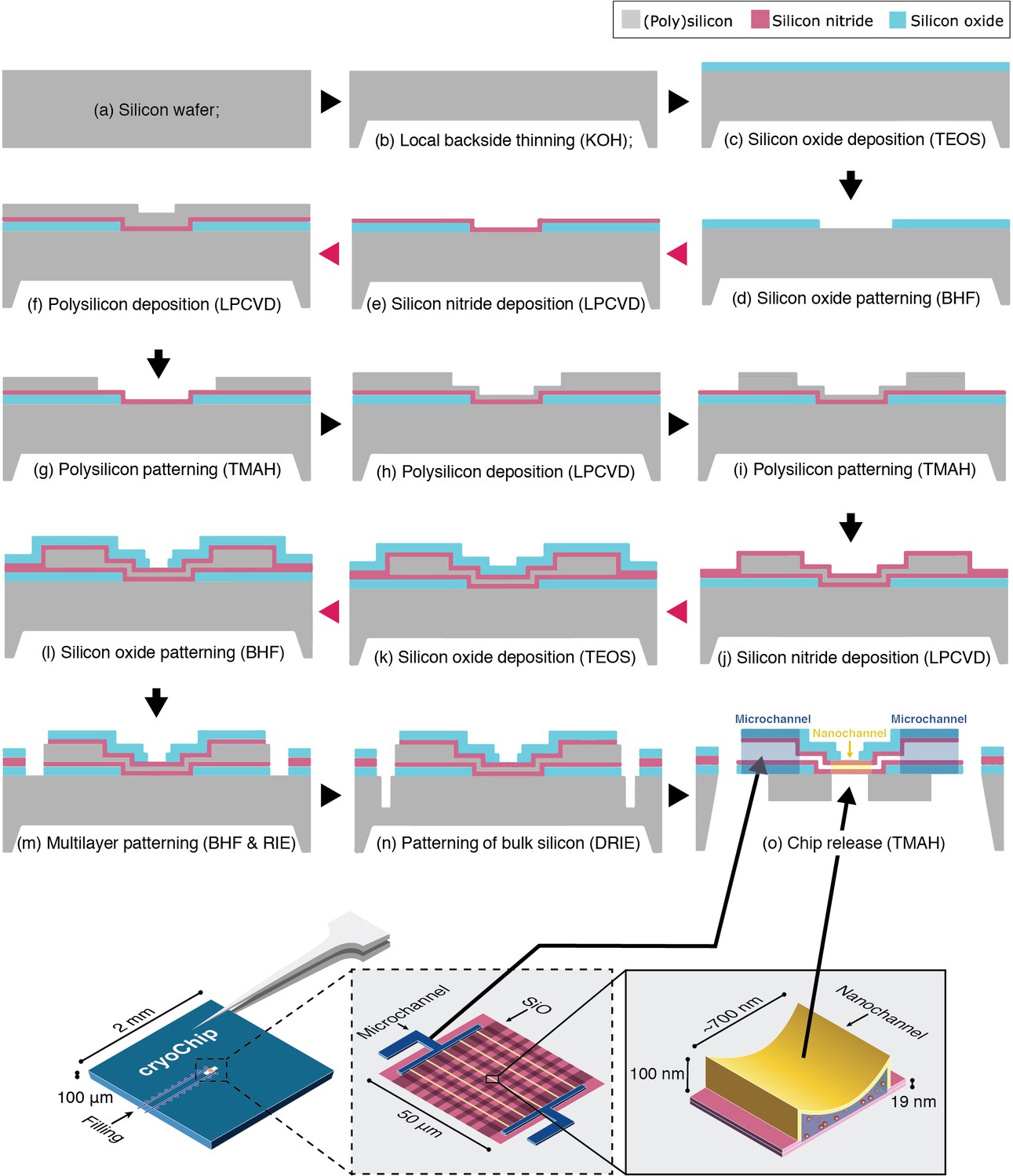
cryoChip fabrication.
Fabrication schematic of cryoChips. All steps for nanofabrication of the cryoChip are shown in cross-section. The graphic on the bottom shows the location of microchannels (supply channels for filling) and nanochannels (for imaging) in the schematic.
Figure 1—figure supplement 2
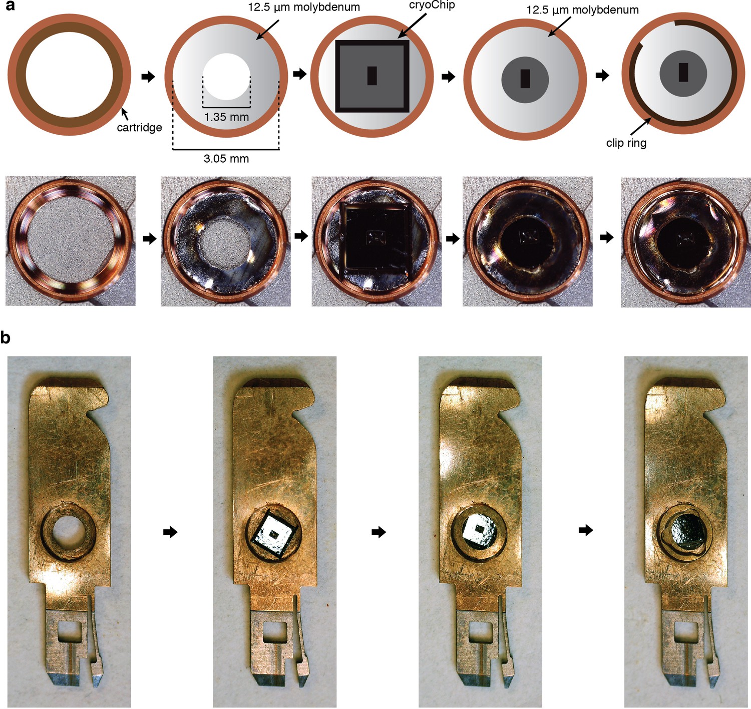
Specimen mounting.
Preparation of cryoChips for TEM imaging. (a) Mounting in Autogrid cartridges (Thermo Fisher Scientific). A cryoChip is sandwiched between two molybdenum adapter rings with a circular aperture (laser cut from 12.5 µm molybdenum foil) and fixated with the Autogrid clip ring. Chips are mounted with the observation membrane facing the cartridge base and the slanted KOH-etch side walls facing the clip ring (b) Mounting in cartridges for the JEOL JEM3200-FSC microscope. The chip is placed with the observation membrane facing the cartridge base. The default metal spacer ring is placed on top and the assembly is secured by a screw ring.
Figure 2 with 7 supplements
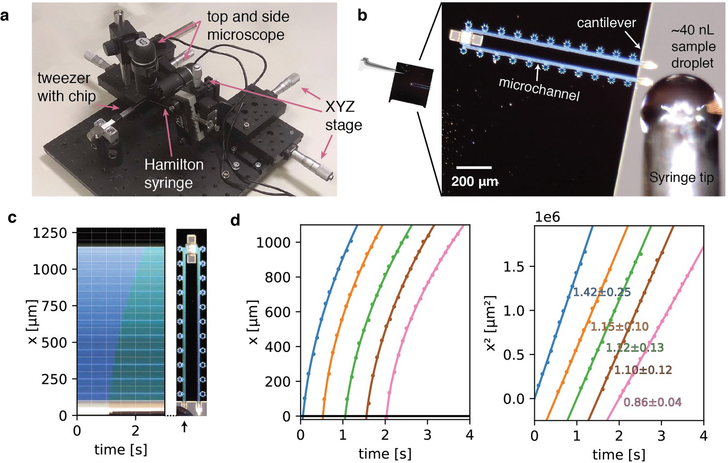
Sample preparation with cryoChips.
(a) Manual filling station with side view and top view microscope, microvolume glass syringe, xyz precision stages for translation of the syringe and a mount for tweezers holding a cryoChip. (b) Sample loading of a cryoChip seen with the top view microscope. One of the cantilevers is approached with a ~40 nL sample droplet. (c) Kymograph of the filling process showing the progression of the sample meniscus over time. The arrow indicates the cantilever and the supply channel. (d) Filling kinetics of cryoChips. The meniscus position and associated time value were recorded at 10 fps with the top-view microscope, revealing a decreasing filling rate with progression of the fluid front (left panel). Each graph represents data from one filling experiment. Graphs from individual experiments are spaced apart by 0.5 s for better visualisation. The squared meniscus position (right panel) displays a linear relationship with elapsed filling time in agreement with expectation from Washburn kinetics. Solid lines are non-linear fits to the data. Slopes (106 μm2/s) and their standard deviations from bootstrapping statistics are shown.
Figure 2—figure supplement 1
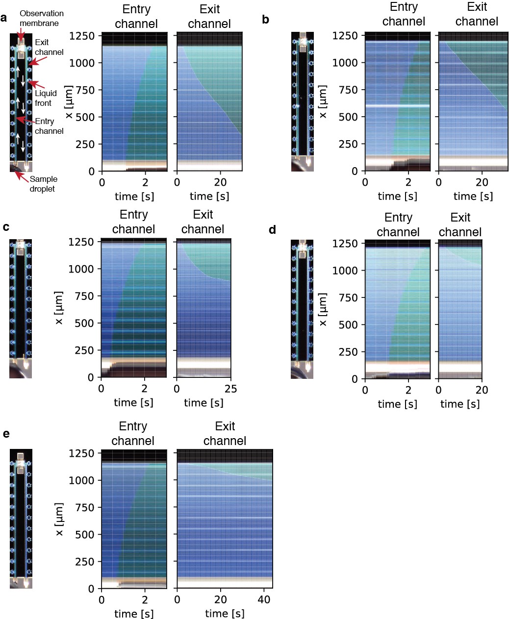
Filling kymographs.
Kymographs showing liquid entry and exit through the supply- and exit microchannels. The liquid takes around one second to flow from the cantilever inside the whole entry channel. Due to the small cross-section of the nanochannels in the observation membrane, liquid flows out of the exit channel very slowly.
Figure 2—video 1
Demonstration of cryoChip filling.
Figure 2—video 2
Raw movie for kymograph (a).
Figure 2—video 3
Raw movie for kymograph (b).
Figure 2—video 4
Raw movie for kymograph (c).
Figure 2—video 5
Raw movie for kymograph (d).
Figure 2—video 6
Raw movie for kymograph (e).
Figure 3
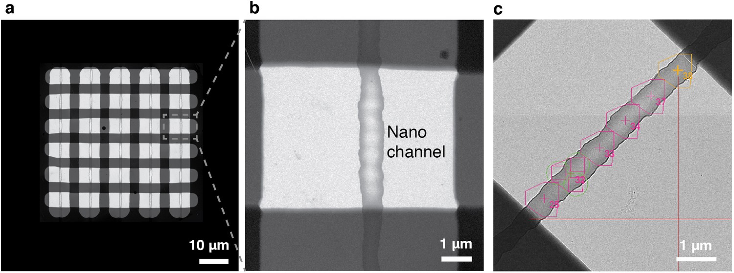
Automated data acquisition with cryoChips.
(a) TEM image of the observation membrane with five nanochannels. The checkerboard structure is a stiffening layer made from silicon oxide that divides the nanochannels in observation windows. (b) Close-up of inset in (a). (c) Medium magnification image of an observation square with an overlay of the SerialEM multishot acquisition scheme containing six acquisition points along the nanochannel. Each acquisition point is centered on a polygon outlining the limits of three imaging positions achieved by beam-image shift, leading to a total of 18 images per observation square.
Figure 4 with 7 supplements
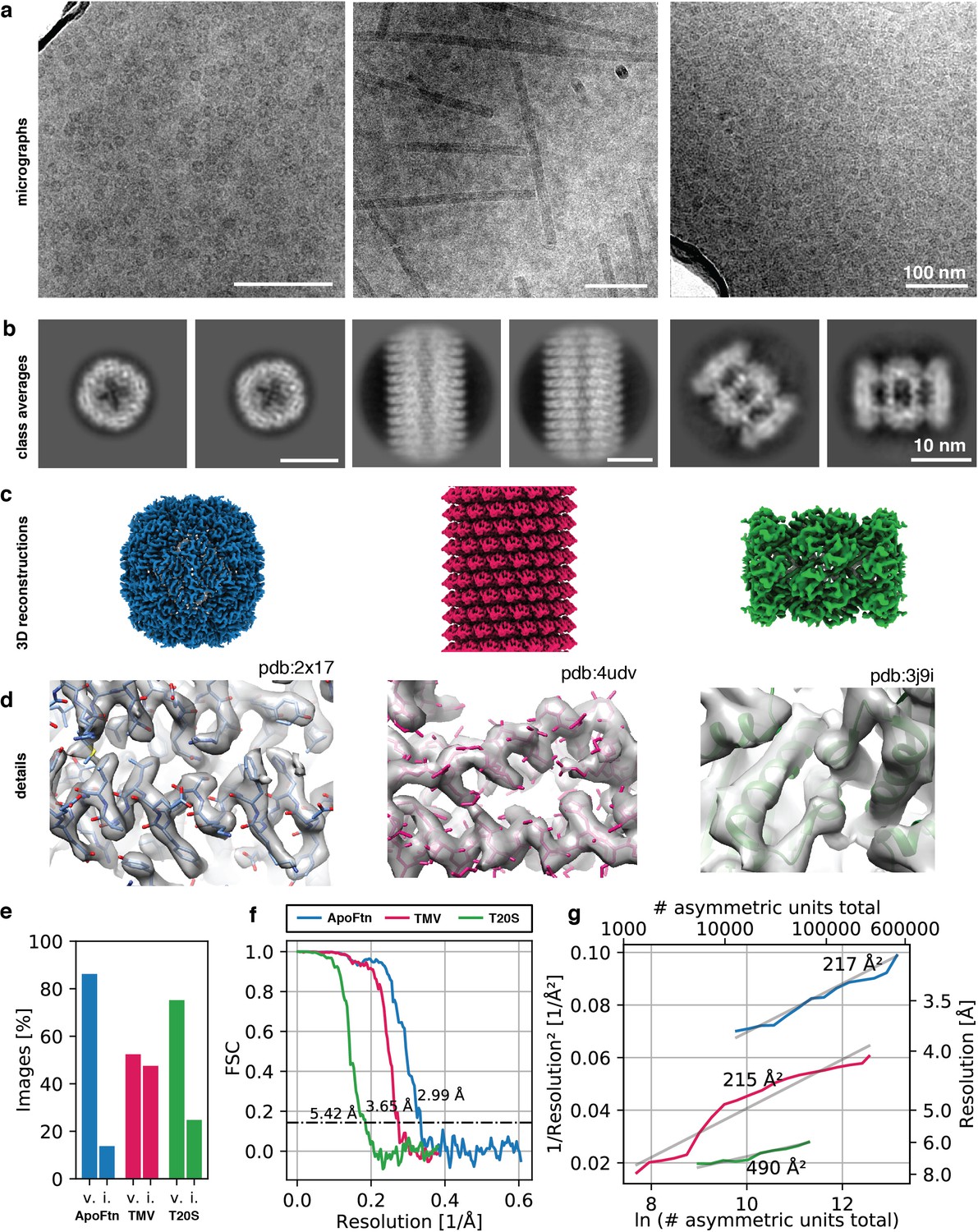
3D reconstruction of ApoFtn, T20S proteasome and TMV.
(a) Raw micrographs, (b) 2D class averages, (c) 3D cryo-EM maps and (d) close-up densities displaying discernible details for the three test specimens. Atomic models were overlaid as visual aid: ApoFtn pdb:2×17 (Kasyutich et al., 2010), TMV pdb:4udv (Fromm et al., 2015), T20S pdb:3j9i (Li et al., 2013) (e) Percentage of images in the dataset classified as vitreous (v) and icy (i). (f) Fourier Shell Correlation (FSC) curves with 0.143 cutoff. (g) ResLog plots for reconstructions. B-factors were estimated as two over the fitted slope. Colour coding is equivalent for panels (c–g). Micrographs in (a) were taken at a defocus of –1.2 µm for ApoFtn, –1.8 µm for TMV and –2.8 µm for T20S. Scale bars are equivalent for images in (a) and class averages in (b).
-
Figure 4—source data 1
Raw data for vitrification statistics.
- https://cdn.elifesciences.org/articles/72629/elife-72629-fig4-data1-v1.txt
-
Figure 4—source data 2
Raw data Fourier Shell Correlation (FSC) curve for ApoFtn dataset.
- https://cdn.elifesciences.org/articles/72629/elife-72629-fig4-data2-v1.txt
-
Figure 4—source data 3
Raw data Fourier Shell Correlation (FSC) curve for T20S dataset.
- https://cdn.elifesciences.org/articles/72629/elife-72629-fig4-data3-v1.txt
-
Figure 4—source data 4
Raw data Fourier Shell Correlation (FSC) curve for TMV dataset.
- https://cdn.elifesciences.org/articles/72629/elife-72629-fig4-data4-v1.txt
-
Figure 4—source data 5
Raw data B-factor plot for T20S dataset.
- https://cdn.elifesciences.org/articles/72629/elife-72629-fig4-data5-v1.txt
-
Figure 4—source data 6
Raw data B-factor plot for TMV dataset.
- https://cdn.elifesciences.org/articles/72629/elife-72629-fig4-data6-v1.txt
-
Figure 4—source data 7
Raw data for COMSOL simulation.
- https://cdn.elifesciences.org/articles/72629/elife-72629-fig4-data7-v1.txt
Figure 4—figure supplement 1
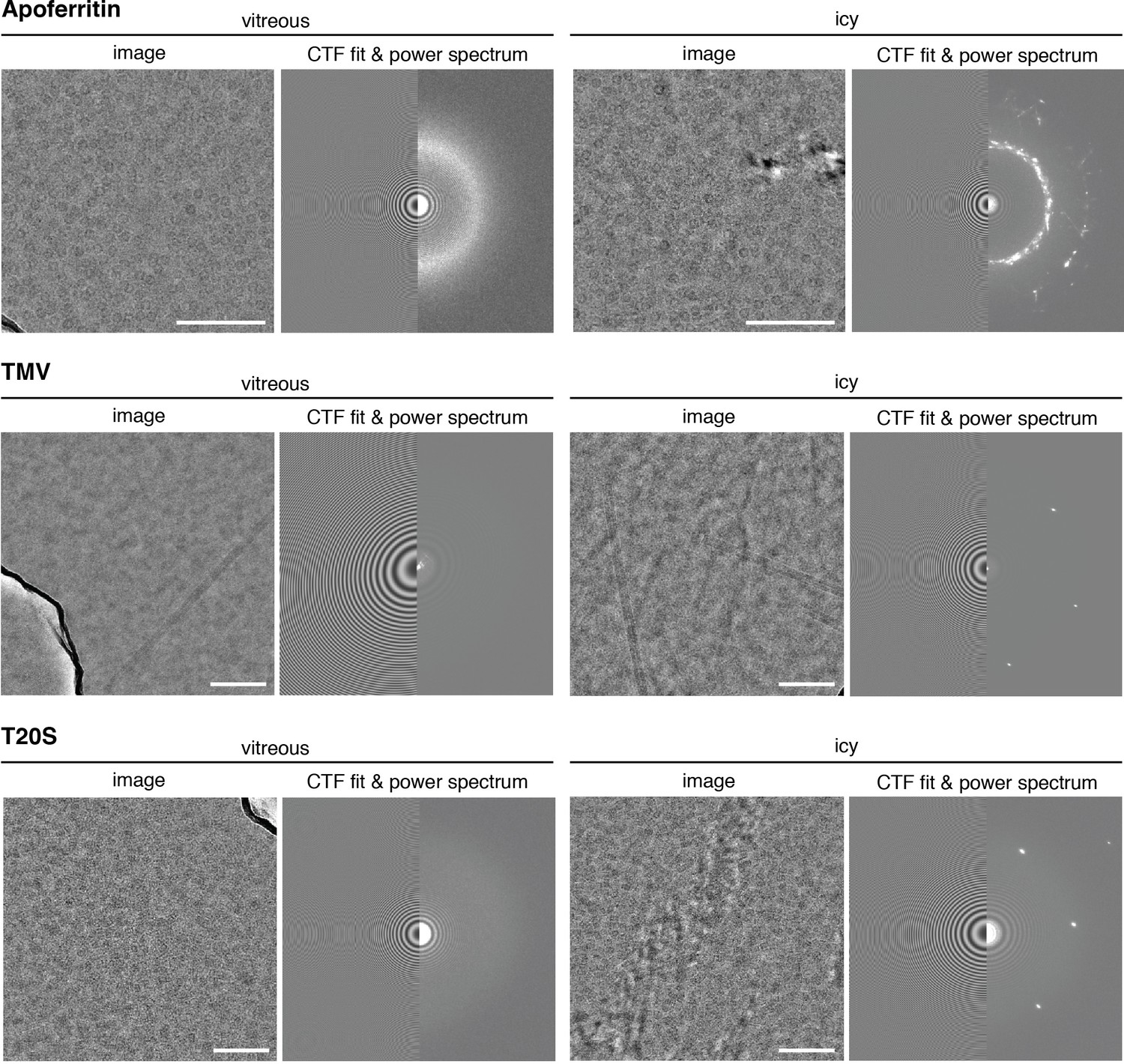
Vitrification efficiency.
Vitrification efficiency analysis. Representative images with vitreous ice (left panels) and crystalline ice (right panels) from the three test specimens. CTF fits to the power spectra are also shown. Thon rings from SiNx can be used for coma-free alignment. Scale bar is 100 nm.
Figure 4—figure supplement 2
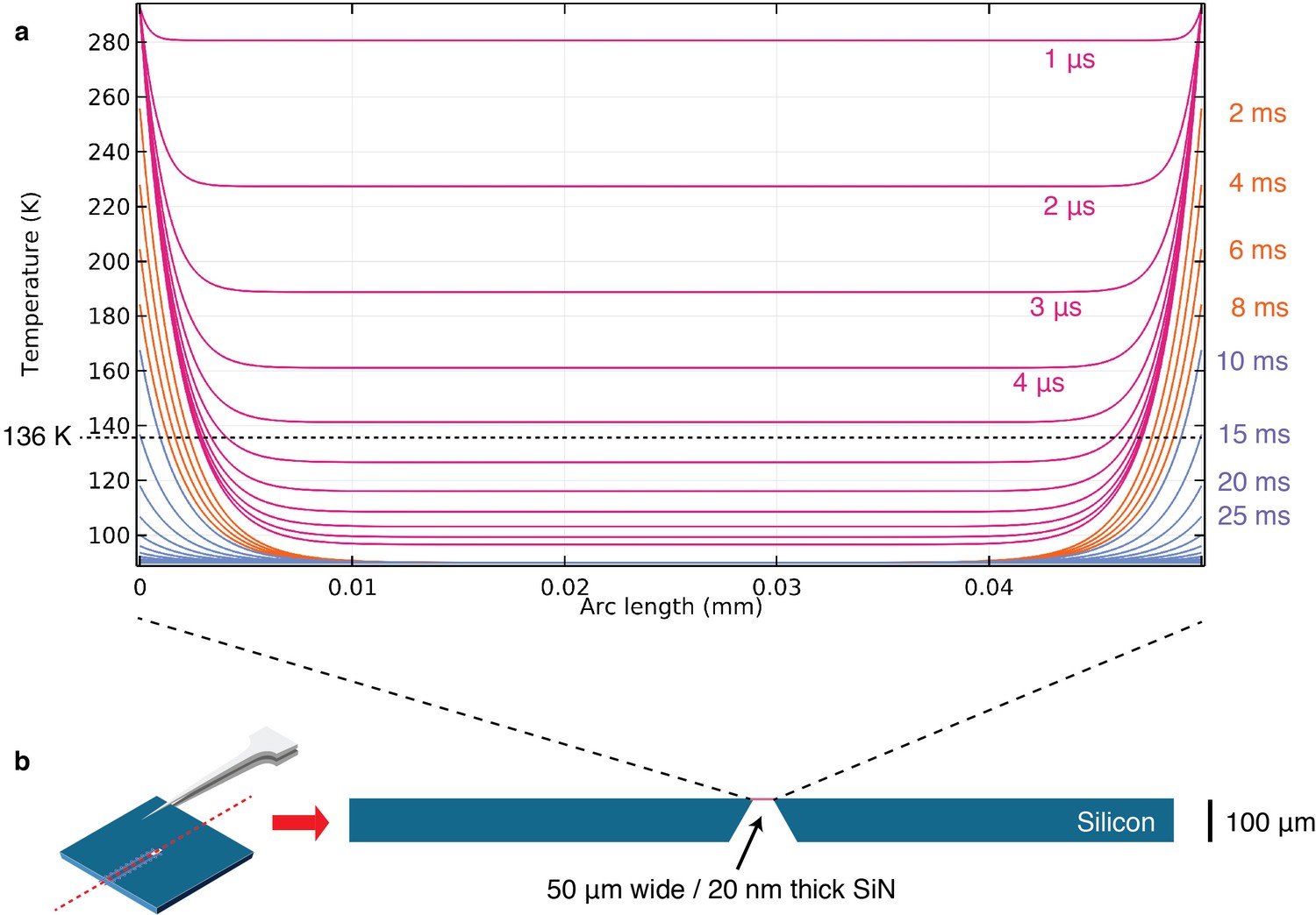
COMSOL simulations.
Simulation of plunge freezing of a simplified model of cryoChips in COMSOL 5.4. (a) Temperature profiles over 50 µm observation membrane from 1-10 µs (pink), 1–10 ms (orange) and 10–100 ms (blue). Dashed line shows glass-transition temperature of water at 136 K. (b) 2D model of cryoChips with 2 mm x 100 µm silicon base and 50 µm x 20 nm SiNx observation membrane used in simulations.
Figure 4—figure supplement 3
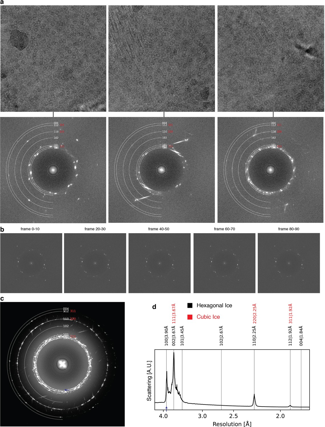
Ice formation.
Analysis of icy micrographs from ApoFtn dataset. (a) Micrograph (top) and power spectrum (bottom) for three examples with crystalline ice. Solid rings indicate expected Bragg spacings diffraction spots for hexagonal ice (white) and cubic ice (red) (derived from Kumai, 2017). (b) Power spectra for frame subsets from the first example in (a) indicate no visible intensity changes of ice reflections throughout the exposure, suggestive of non-vitreous sections in the nanochannels and not surface ice contamination. (c) Maximum intensity projection of all power spectra from the entire ApoFtn dataset. (d) Rotational average of (c) shows four discernible diffraction peaks, including the (100) reflection (3.90 Å) unique for hexagonal ice (blue arrow).
Figure 4—figure supplement 4
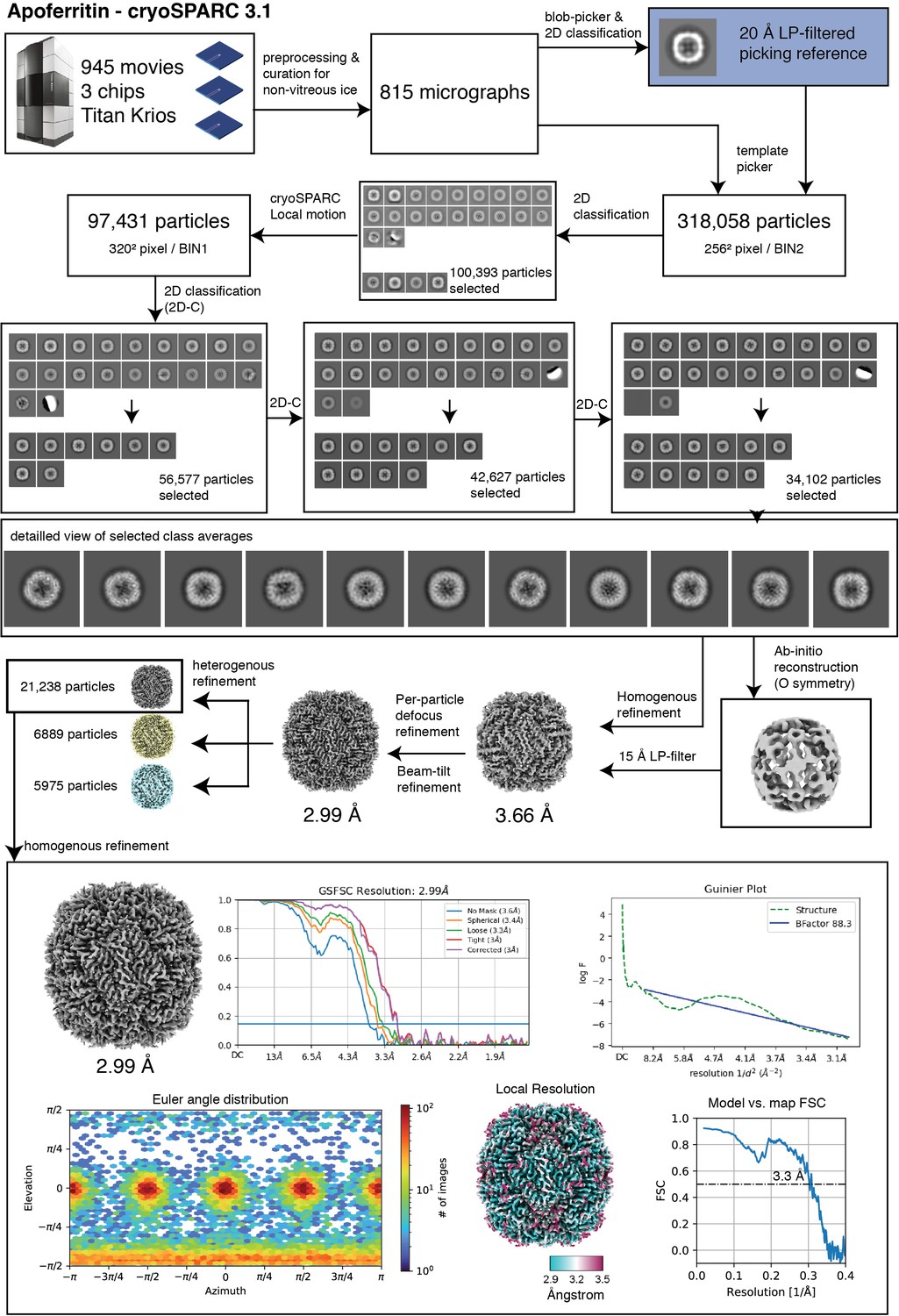
ApoFtn processing.
Single-particle analysis workflow for P. furiosus apoferritin (ApoFtn).
Figure 4—figure supplement 5
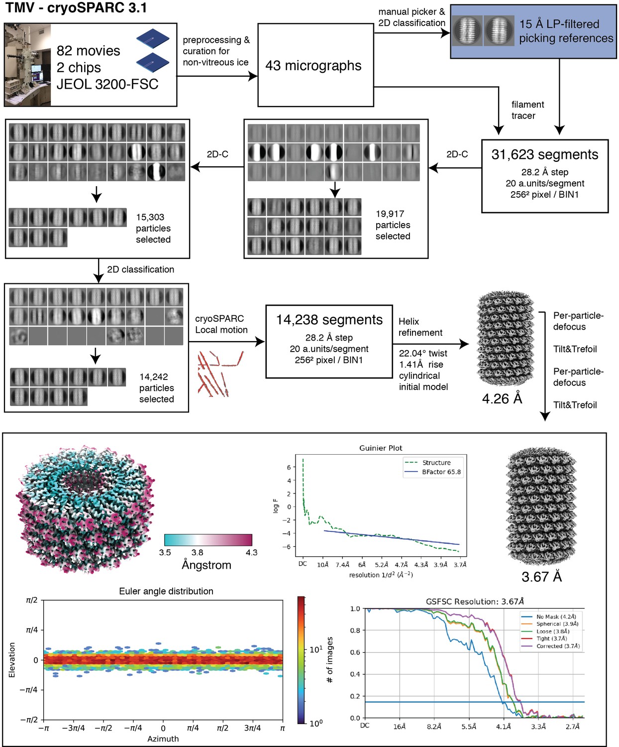
TMV processing.
Single-particle analysis workflow for tobacco mosaic virus (TMV).
Figure 4—figure supplement 6
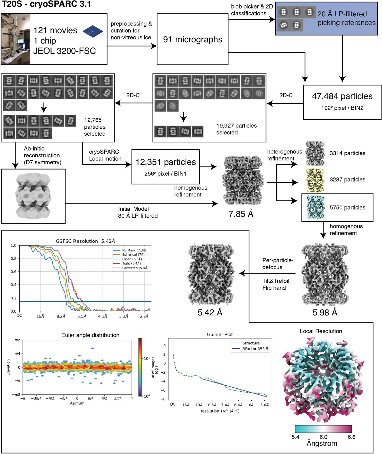
T20S processing.
Single-particle analysis workflow for T. acidophilum T20S proteasome (T20S).
Figure 4—figure supplement 7
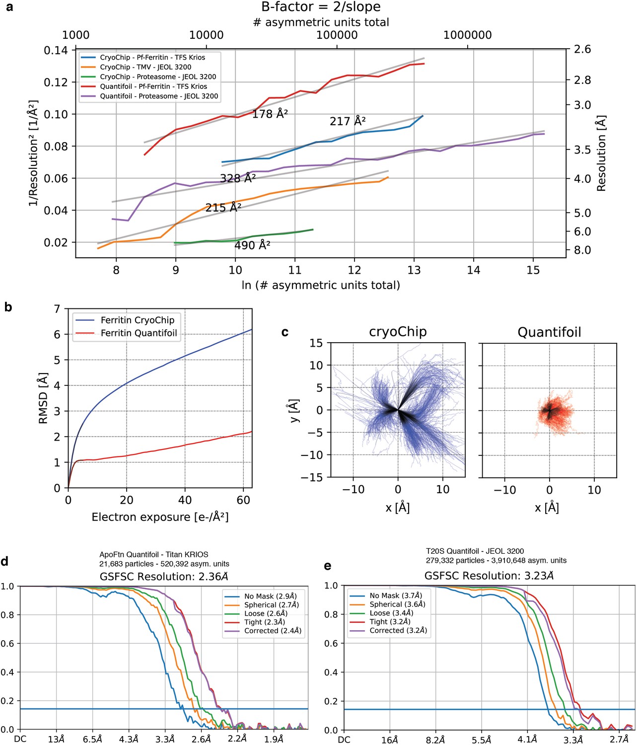
B-factor analysis.
Comparison of cryoChip datasets with reference datasets on conventional holey carbon (QF). (a) B-factor plots for ApoFtn, T20S and TMV from cryoChip and holey carbon (T20S and ApoFtn) datasets obtained using the same acquisition settings and processing workflows. (b) Motion trajectories for ApoFtn datasets from cryoChip and holey carbon grids. The overall specimen movement for cryoChips is higher, but initial movement at 0-5 e-/Å2 is on the order of 0.5 pixel/frame. (c) Trajectories from (b). Fourier Shell Correlation (FSC) curves for 3D reconstructions of (d) ApoFtn and (e) T20S from holey carbon reference datasets. datasets.
Figure 5 with 1 supplement
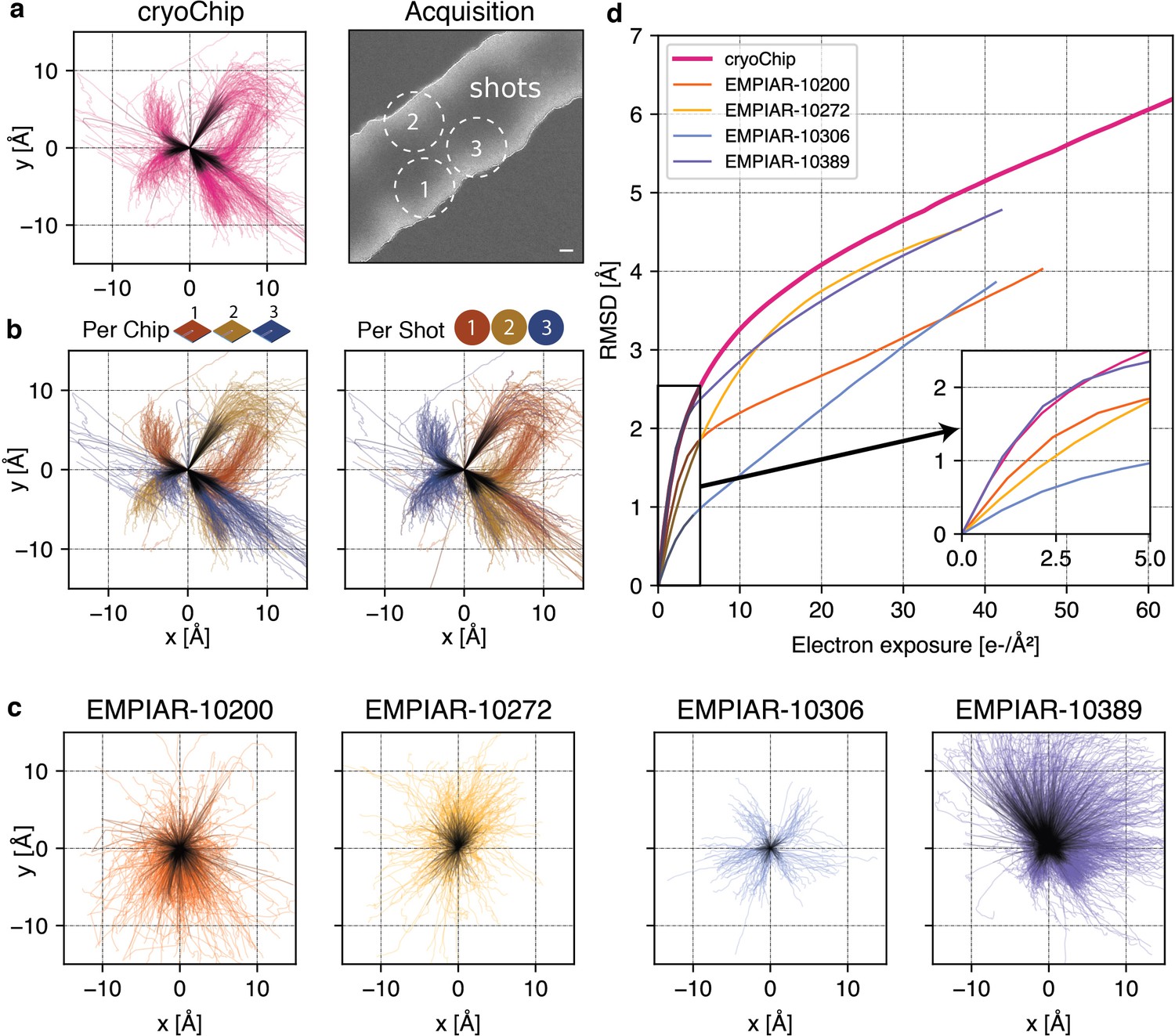
Comparison of beam-induced motion for cryoChip and reference datasets from conventional sample preparation.
(a) Whole-frame motion trajectories of dose-fractionated movies during exposure with 63 e-/Å2 from three different cryoChips. (b) Trajectories coloured by chip or by imaging position in a repeating three-shot pattern. (c) Whole-frame motion trajectories of reference datasets. (d) Root-mean-square deviation (RMSD) of trajectories over electron exposure between the cryoChip dataset and reference datasets. The inset shows the first part of the exposure most critical for reconstructing high-resolution details. Scale bar in (a) is 100 nm. First five e-/Å2 in trajectories are coloured in black.
-
Figure 5—source data 1
Raw motion track data for cryoChip 1,2, and 3.
- https://cdn.elifesciences.org/articles/72629/elife-72629-fig5-data1-v1.zip
-
Figure 5—source data 2
Raw motion track data for EMPIAR 10200, 10272, 10306, 10,389.
- https://cdn.elifesciences.org/articles/72629/elife-72629-fig5-data2-v1.zip
-
Figure 5—source data 3
Raw data for cumulated motion plots.
- https://cdn.elifesciences.org/articles/72629/elife-72629-fig5-data3-v1.zip
Figure 5—figure supplement 1
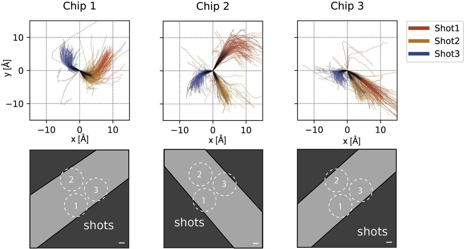
Motion analysis.
Beam-induced motion of ApoFtn dataset in cryoChips. Motion trajectories separated by chip and colour-coded by acquisition location reveal preferred directions of movement specific for each shot position in the nanochannels. Pictograms show the direction of nanochannels in the acquisition movies. Scale bar: 100 nm.
-
Figure 5—figure supplement 1—source data 1
Raw motion track data for Figure 5—figure supplement 1.
- https://cdn.elifesciences.org/articles/72629/elife-72629-fig5-figsupp1-data1-v1.txt
Figure 6 with 4 supplements
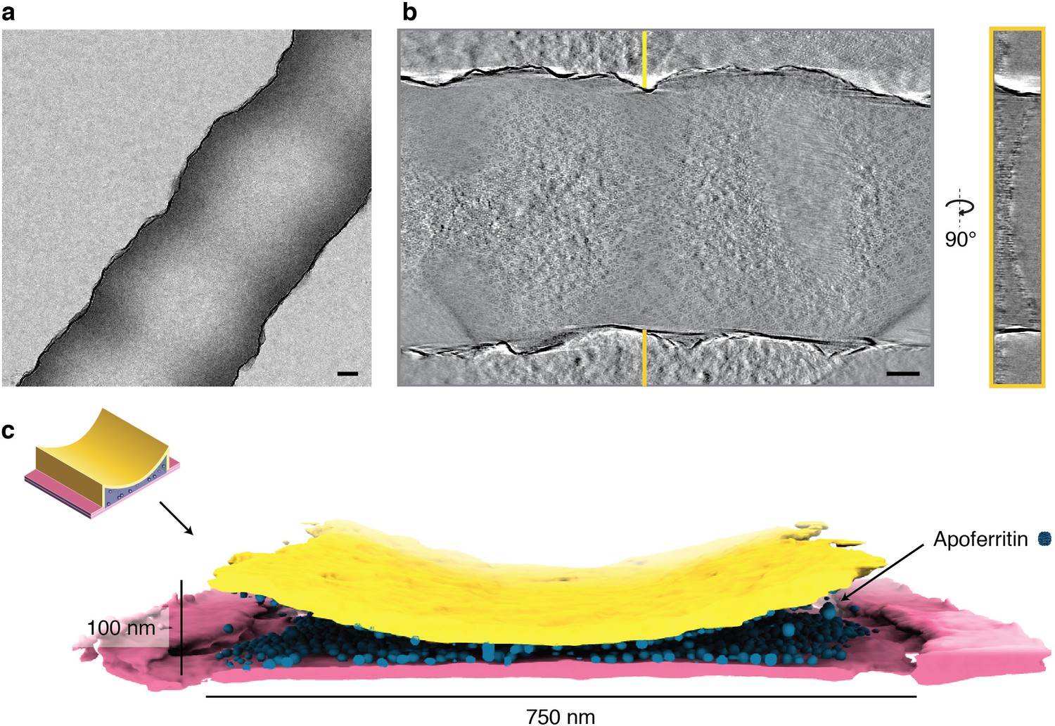
Tomographic reconstruction of a cryoChip nanochannel filled with ApoFtn.
(a) Overview image of tomogram area of a nanochannel segment filled with ApoFtn. (b) Slice through the reconstructed tomogram and yz cross-section across the nanochannel indicated by lines. (c) Segmented reconstruction showing the nanochannel membrane (bottom: pink, top: yellow) and ApoFtn in the channel lumen (blue). The thickness of the membrane is affected by the missing wedge and not to scale. All scale bars: 100 nm.
Figure 6—figure supplement 1

TMV and T20S cryoChip tomograms.
Tomograms of cryoChips with TMV and T20S. (a) Schematic illustration of volume determination and particle counting for a part of the ApoFtn tomogram. Segmented ApoFtn particles are shown as spheres. Low (top) and medium (center) magnification micrographs and segmented tomograms of nanochannels filled with (b) TMV (EMD-12914) and (c) T20S proteasome (EMD-12917). The cryoChip for T20S has a clover-patterned design of nanochannel and circular observation windows.
Figure 6—figure supplement 2
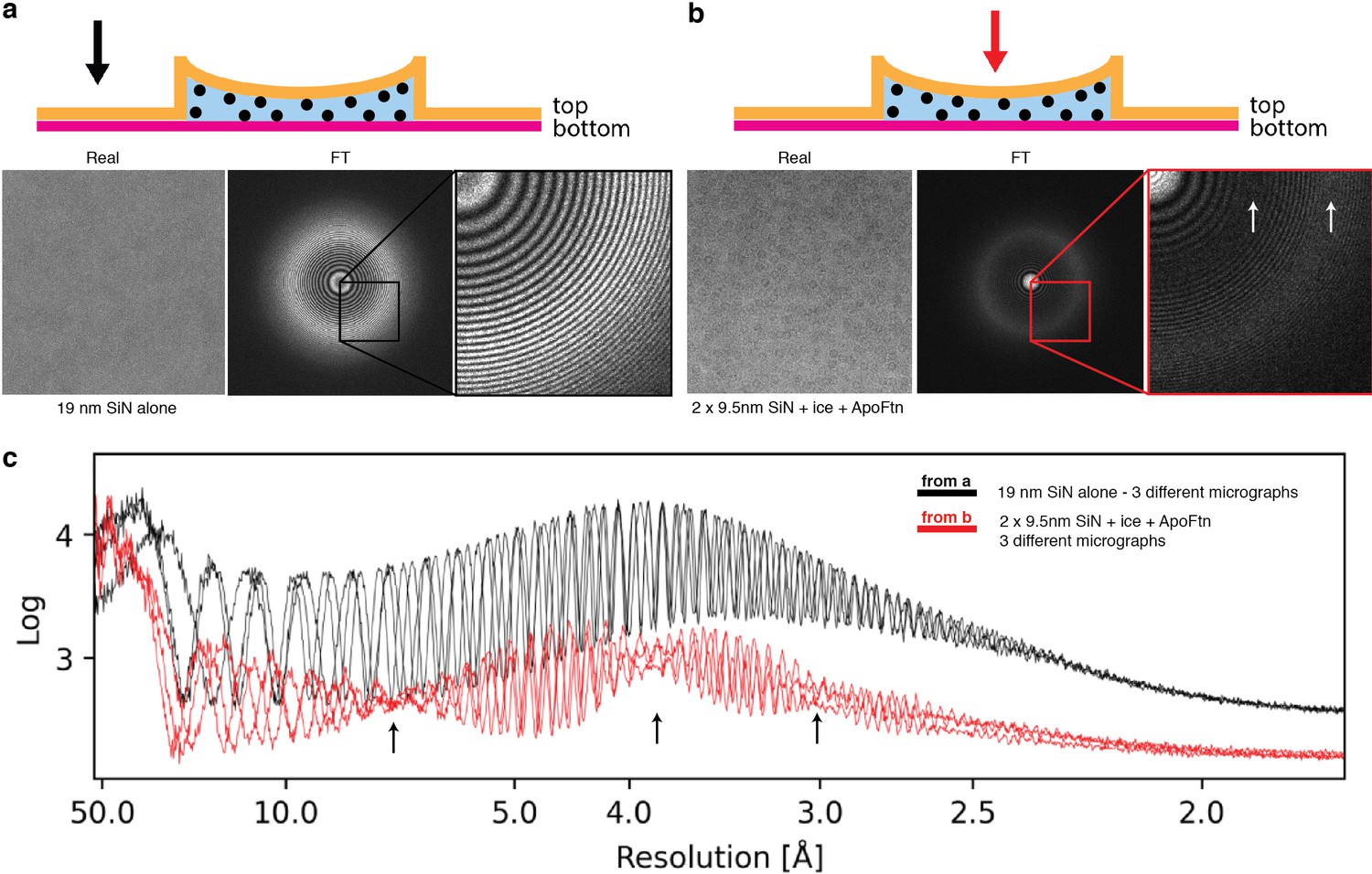
SiN Fourier spectra.
Spectral analysis of SiN. Real space image, Fourier amplitude spectrum and detail of Fourier amplitude spectrum for (a) 19 nm silicon nitride membrane adjacent to a nanochannel (b) ApoFtn in vitreous ice in a silicon nitride nanochannel. Arrows in the schematics indicate imaging position. The top and bottom membrane of the nanochannel are between 0 and 100 nm apart, leading to interference of their CTFs resulting in nodes (arrows) in their overall Thon ring pattern. (c) Radially averaged power spectra of three micrographs at different defoci show a broad peak of scattering intensity for amorphous SiN at about 3.9 Å. CTF nodes are visible in the nanochannel Fourier spectra (arrows).
Figure 6—figure supplement 3
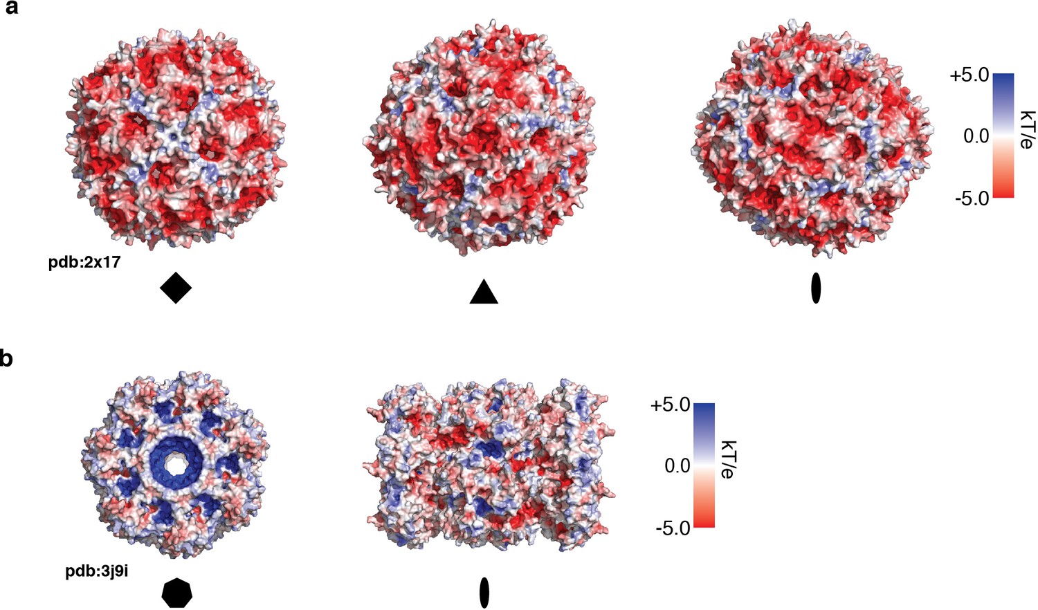
Surface electrostatic potential maps.
Electrostatic potential maps for (a) ApoFtn, displayed along fourfold, threefold, and twofold axes and (b) T20S proteasome displayed along the sevenfold and twofold axes. Electrostatic potentials have been computed from PDB ID 2×17 (Kasyutich et al., 2010) and PDB ID 3j9i (Li et al., 2013) using the Adaptive Poisson Boltzmann server (ABPS) (Jurrus et al., 2018).
Figure 6—video 1
Zoom-in video of cryoChip.
Tables
Key resources table
| Reagent type (species) or resource | Designation | Source or reference | Identifiers | Additional information |
|---|---|---|---|---|
| Gene (P. furiosus) | Ferritin | Gift from Carsten Sachse | Uniprot ID:Q8U2T8 | |
| Gene (T. acidophilium) | T20S proteasome | Gift from Yifan Cheng | Addgene ID:110805 | |
| Software, algorithm | cryoSPARC | Punjani et al., 2017 PMID:28165473 | RRID:SCR_016501 v3.1 | |
| Software, algorithm | UCSF ChimeraX | Goddard et al., 2018 PMID:28710774 | RRID:SCR_015872v1.2 | |
| Software, algorithm | Coot | Emsley et al., 2010 PMID:20383002 | RRID:SCR_014222v0.8.9.2 | |
| Software, algorithm | Phenix | Adams et al., 2010 PMID:20124702 | RRID:SCR_014224v1.13 | |
| Software, algorithm | MOLPROBITY | Chen et al., 2010 PMID:20057044 | RRID:SCR_014226v1.17.1 | |
| Software, algorithm | MotionCor2 | Zheng et al., 2017 PMID:28250466 | RRID:SCR_016499v1.0 | |
| Software, algorithm | IMOD | Mastronarde and Held, 2017 PMID:2744392 | RRID:SCR_003297v4.9.12 |
Additional files
-
Transparent reporting form
- https://cdn.elifesciences.org/articles/72629/elife-72629-transrepform1-v1.pdf
-
Supplementary file 1
Data collection and refinement statistics for collected datasets.
- https://cdn.elifesciences.org/articles/72629/elife-72629-supp1-v1.pdf
-
Supplementary file 2
Data collection and refinement statistics for reference datasets on holey carbon grids.
- https://cdn.elifesciences.org/articles/72629/elife-72629-supp2-v1.pdf
-
Supplementary file 3
Model refinement statistics for ApoFtn atomic model.
- https://cdn.elifesciences.org/articles/72629/elife-72629-supp3-v1.pdf
-
Supplementary file 4
Data and 3D reconstruction parameters of reference datasets.
- https://cdn.elifesciences.org/articles/72629/elife-72629-supp4-v1.pdf
Download links
A two-part list of links to download the article, or parts of the article, in various formats.
Downloads (link to download the article as PDF)
Open citations (links to open the citations from this article in various online reference manager services)
Cite this article (links to download the citations from this article in formats compatible with various reference manager tools)
Nanofluidic chips for cryo-EM structure determination from picoliter sample volumes
eLife 11:e72629.
https://doi.org/10.7554/eLife.72629


