Research Article

Epidemiology and Global Health

Linking rattiness, geography and environmental degradation to spillover Leptospira infections in marginalised urban settings: An eco-epidemiological community-based cohort study in Brazil

Centre for Health Informatics, Computing, and Statistics, Lancaster University Medical School, United Kingdom
Liverpool School of Tropical Medicine, United Kingdom
Institute of Collective Health, Federal University of Bahia, Brazil
Swedish University of Agricultural Sciences, Sweden
Oswaldo Cruz Foundation, Brazilian Ministry of Health, Brazil
Department of Epidemiology of Microbial Diseases, Yale School of Public Health, United States
University of Pennsylvania, United States
World Health Organization (WHO) Regional Office for Europe, Denmark
Department of Evolution, Ecology and Behaviour, University of Liverpool, United Kingdom

Sep 16, 2022

https://doi.org/10.7554/eLife.73120

Open access
Copyright information

Figures
Tables
Additional files

9 figures, 8 tables and 2 additional files

Figures

Figure 1

Download asset Open asset

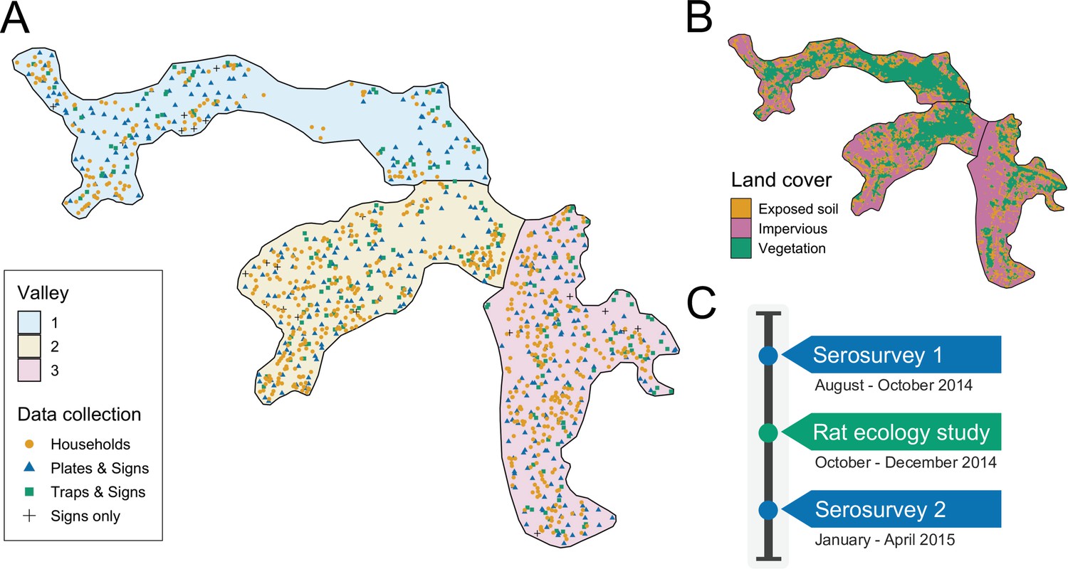
Study site and timeline.

(A) Map of the three valleys within the study site in Pau da Lima, with household locations for the serosurveys marked as orange circles. Locations sampled in the the rat ecology study are shown for each of the rat abundance indices as follows: Plates & Signs (track plates, burrows, faeces and trails), Traps & Signs (traps, burrows, faeces and trails) and Signs only (burrows, faeces, and trails); (B) Land cover classification map (impervious cover is defined as man-made structures e.g. pavement and buildings); (C) Study timeline for the two community serosurveys and rat ecology study.

Figure 2

Download asset Open asset

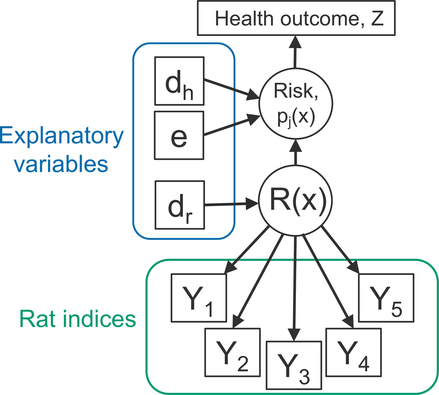
Directed acyclic graph (DAG) of the rattiness-infection model framework.

$R (x)$ is the value of a spatially continuous stochastic rattiness process at location $x$ . The outcome variables $Y_{k} : k = 1, \dots, 5$ are the set of five rat abundance indices that provide information about $R (x)$ : traps ( $k = 1$ ), track plates ( $k = 2$ ), number of burrows ( $k = 3$ ), presence of faecal droppings ( $k = 4$ ) and presence of trails ( $k = 5$ ). The outcome variable $Z_{i, j}$ is the observed health outcome, in this case this represents infection status. The terms d_h and d_r represent the sets of spatially continuous explanatory variables which contribute to spatial variation in infection risk in humans and $R (x)$ , respectively. The terms d_h and d_r are not mutually exclusive groups of explanatory variables and the same variables may contribute to both infection risk and $R (x)$ . The term $e$ represents a set of individual- and household-level explanatory variables which contribute to variation in infection risk. Square objects correspond to observable variables, and circles to latent random variables.

Figure 3

Download asset Open asset

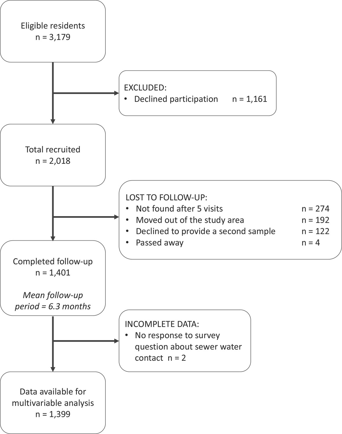
The study participant flow chart in line with the STROBE (Strengthening the Reporting of Observational Studies in Epidemiology) statement (http://www.strobestatement.org).

Figure 4

Download asset Open asset

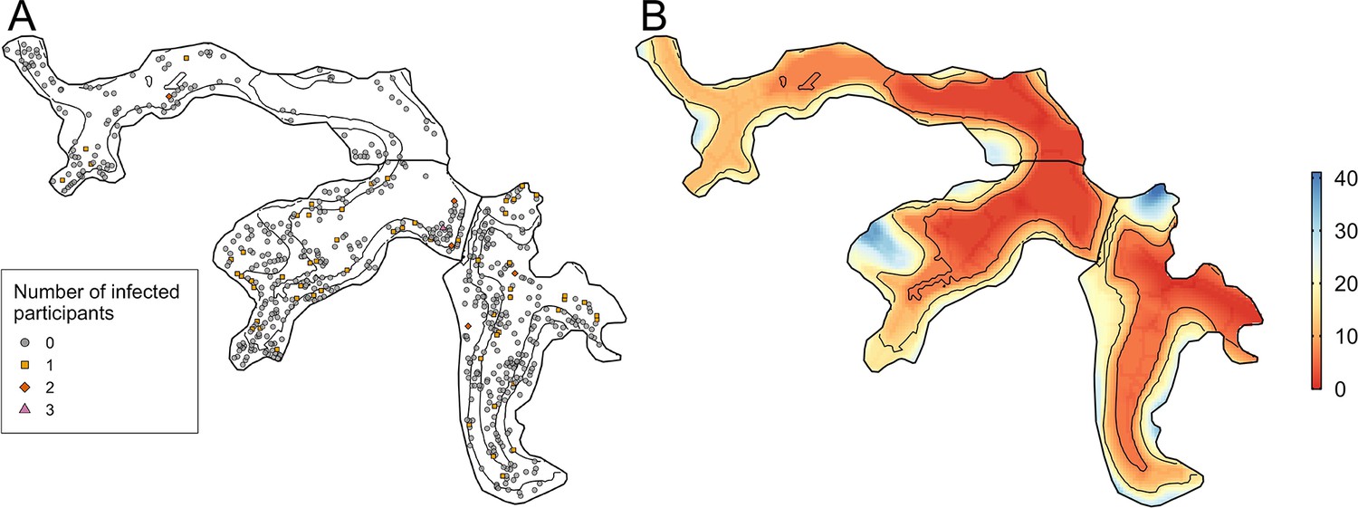
Household infection and elevation maps.

(A) Map of participant household locations with the number of leptospiral infections in each household marked (grey circle - no infections; orange square - 1 infection; red diamond - 2 infections; pink triangle - 3 infections) and contours marking low, medium, and high relative elevation category; (B) Elevation (metres) relative to the bottom of the valley with contours marking low, medium, and high relative elevation levels.

Figure 5

Download asset Open asset

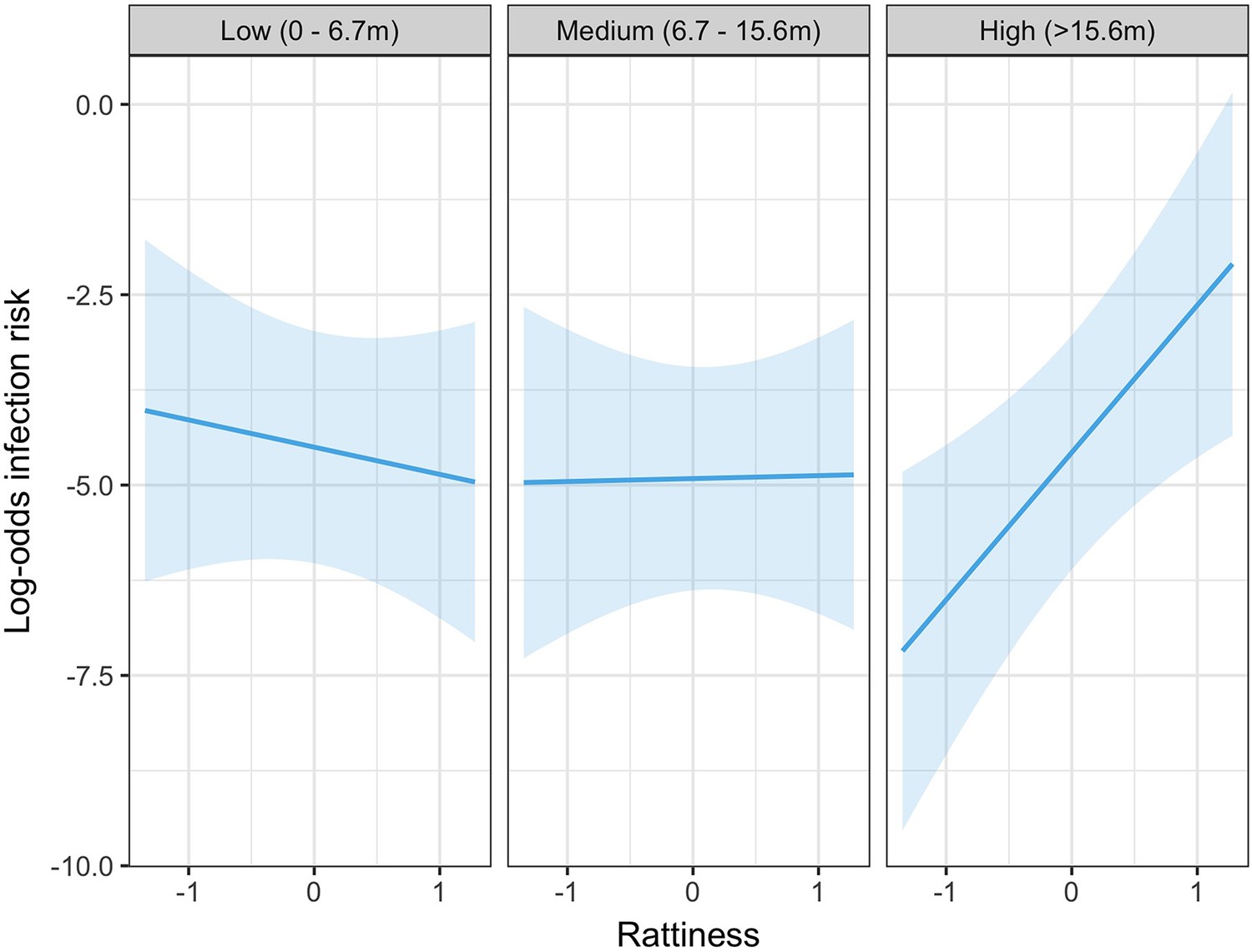
Predicted relationship between rattiness and infection risk from the multivariable mixed effects logistic regression demonstrating evidence of an interaction with relative elevation category (low, medium and high).

Shown on the log-odds scale with shaded areas corresponding to 95% confidence intervals.

Figure 6

Download asset Open asset

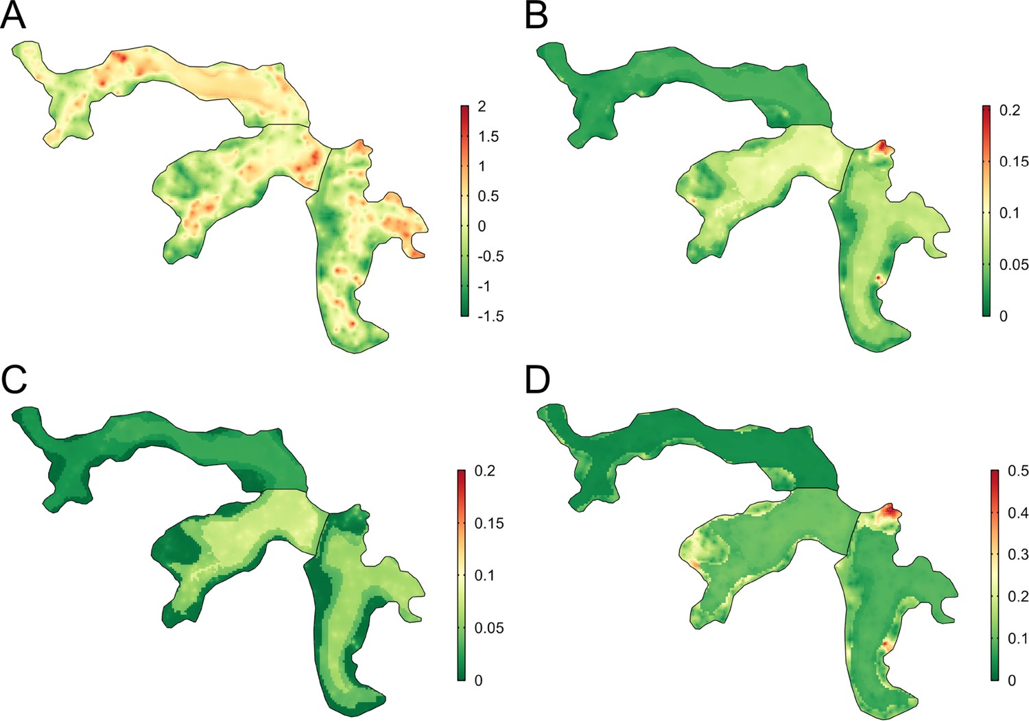
Joint rattiness-infection model predictions.

(A) Mean predicted rattiness; (B) Mean predicted leptospiral infection risk for 30-year-old male participants with a household per capita income of USD$1 /day who never/rarely have contact with floodwater and do not work as a travelling salesperson; (C) lower 95% prediction interval for predicted infection risk; (D) upper 95% prediction interval for predicted infection risk.

Appendix 1—figure 1

Download asset Open asset

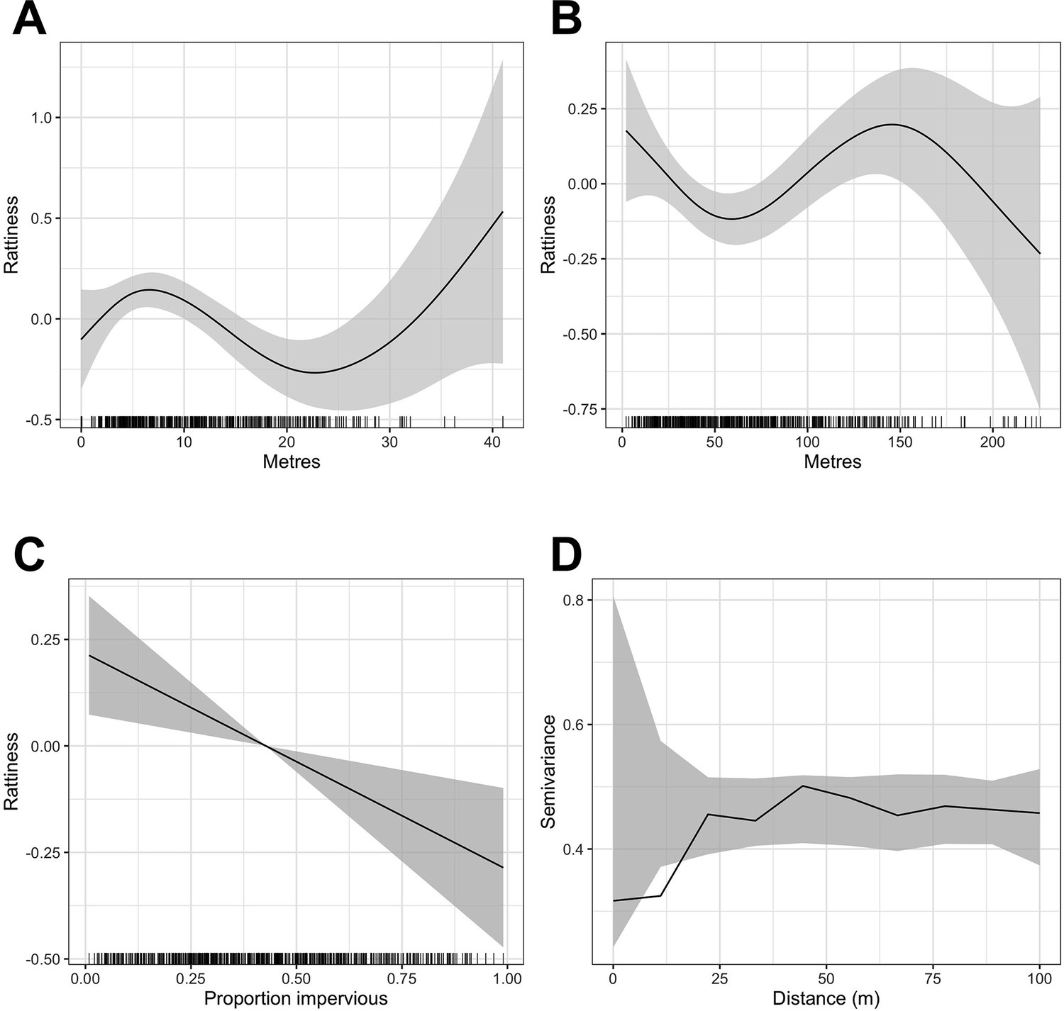
Generalized Additive Model (GAM) partial dependence plots for the unstructured random variation in rattiness,, ${\hat{U}}_{i}$ plotted against the continuous explanatory variables considered in the analysis (shaded areas correspond to 95% confidence intervals).

(A) elevation relative to the bottom of valley, (B) distance to large refuse piles, (C) impervious land cover in 20 m radius buffer around sampling point. are estimated using a non-spatial model which excludes all covariates. (D) is a variogram computed from ${\hat{U}}_{i}$ using a non-spatial model that includes all of the covariates; the dashed lines correspond to 95% confidence intervals under the assumption of spatial independence.

Appendix 1—figure 2

Download asset Open asset

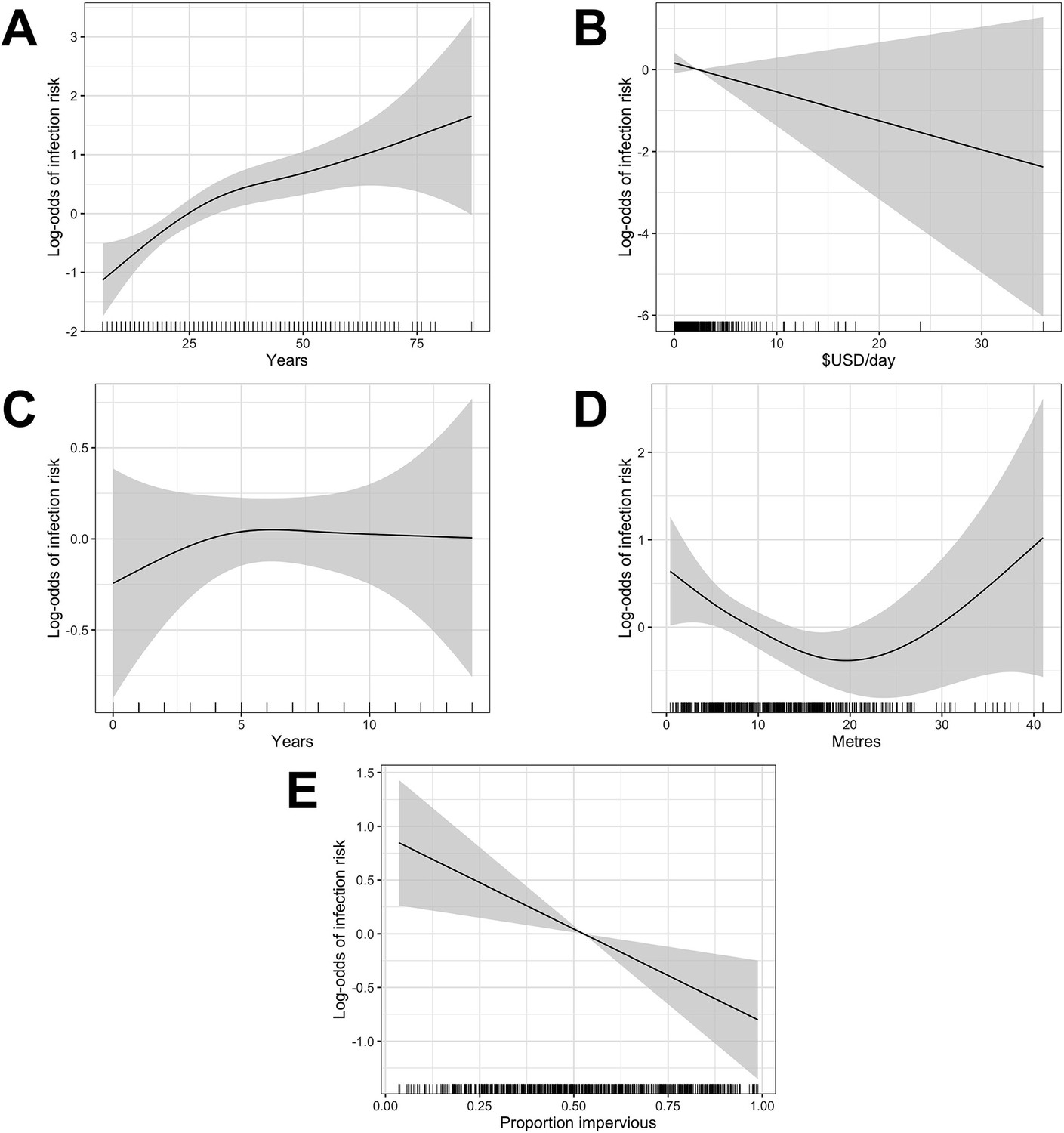
Generalized Additive Model (GAM) partial dependence plots for human infection risk plotted against the continuous explanatory variables considered in this analysis (shaded areas correspond to 95% confidence intervals).

(A) age, (B) household per capita income (in USD), (C) years of education, (D) household elevation relative to the bottom of valley, (E) impervious land cover in 20 m radius buffer around household.

Appendix 7—figure 1

Download asset Open asset

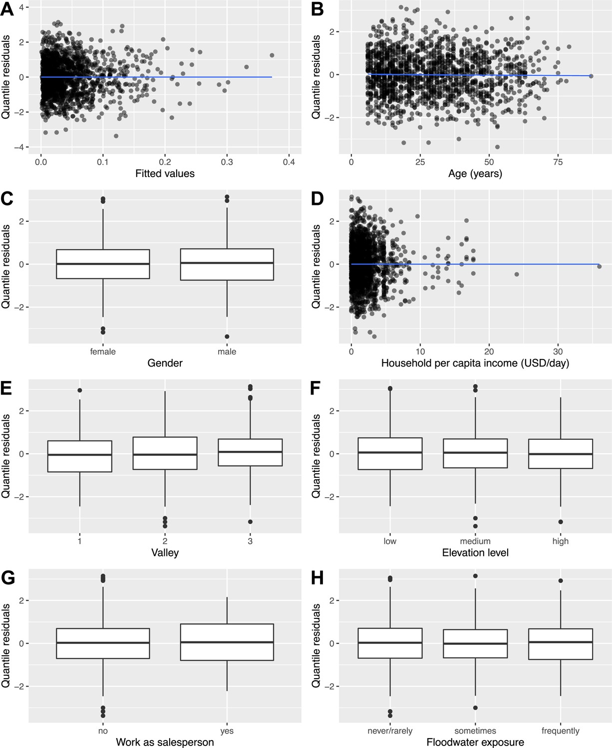
Residual diagnostic plots showing randomised quantile residuals plotted against: (A) fitted values; (**B–H**) variables in the model.

Tables

Table 1

Multivariable linear regression analysis of predictors for rattiness (note that rattiness is a unit-variance random variable when interpreting the magnitude of effect estimates).

Variable	Estimate (95% CI) *
Relative elevation (per 1 m increase)^†
0–8 m	0.04 (0.00, 0.07)
8–22 m	–0.04 (-0.09, 0.01)
>22 m	0.06 (0.00, 0.10)
Distance to large refuse piles (per 10 m increase)^†
0–50 m	–0.07 (-0.13,–0.01)
>50 m	0.02 (-0.05, 0.09)
Impervious land cover (per 10% increase)	–0.05 (-0.08,–0.01)

*

CI, Confidence interval.
†

The effects of relative elevation and distance to refuse are modelled as broken linear models with transitions at 8m and 22m, and 50m, respectively. This was informed by the relationship described by Generalized Additive Modelling in Appendix 1—figure 1.

Table 2

Univariable mixed effects logistic regression analysis of human risk factors for leptospiral infection.

Variable	OR (95% CI)*	aOR (95% CI)*
Demographic and social status
Age (per year)^†
0–30 years old	1.08 (1.03, 1.13)	1.09 (1.04, 1.15)
>30 years old	1.02 (0.96, 1.09)	1.02 (0.95, 1.08)
Male gender	2.22 (1.31, 3.85)	2.78 (1.56, 4.96)
Daily per capita household income (US$/day)	1.01 (0.89, 1.11)	0.92 (0.80, 1.05)
Valley
1	REF	REF
2	3.35 (1.33, 10.37)	3.52 (1.23, 10.05)
3	2.39 (0.93, 7.38)	2.53 (0.88, 7.27)
Adult illiteracy	1.34 (0.61, 2.79)	0.66 (0.29, 1.49)
Education (per year of education)^†
0–5 years	1.05 (0.85, 1.32)	1.14 (0.91, 1.44)
>5 years	0.96 (0.73, 1.27)	0.96 (0.75, 1.26)
Household environment
Impervious land cover (per 10% increase)	0.87 (0.76, 0.99)	0.82 (0.71, 0.95)
Relative elevation (per 1 m increase)^†
0–20 m	0.94 (0.89, 0.99)	0.93 (0.88, 0.99)
>20 m	1.12 (0.98, 1.29)	1.12 (0.97, 1.29)
Relative elevation category ^‡
Low (0–6.7 m)	REF	REF
Medium (6.7–15.6 m)	0.72 (0.37, 1.39)	0.72 (0.36, 1.44)
High (>15.6 m)	0.58 (0.27, 1.20)	0.51 (0.23, 1.11)
Open sewer within 10 m	1.60 (0.85, 3.17)	1.69 (0.85, 3.37)
Unprotected from open sewer	1.00 (0.55, 1.79)	1.11 (0.61, 2.03)
Live on hillside	0.99 (0.52, 1.86)	0.89 (0.46, 1.71)
Occupational exposures
Work in construction ^§	1.36 (0.51, 3.21)	0.62 (0.23, 1.67)
Work as travelling salesperson ^§	4.81 (1.12, 18.78)	2.97 (0.71, 12.40)
Work in refuse collection ^§	2.95 (1.04, 7.89)	1.57 (0.56, 4.42)
Work involves contact with floodwater ^§	0.89 (0.04, 5.61)	0.52 (0.05, 4.96)
Work involves contact with sewer water ^§	3.61 (0.45, 20.38)	1.92 (0.29, 12.80)
Behavioural exposures
Contact with floodwater in last 6 months
Never/rarely	REF	REF
Sometimes	0.61 (0.27, 1.25)	0.66 (0.30, 1.47)
Frequently	2.14 (0.91, 4.94)	2.84 (1.18, 6.86)
Contact with sewer water in last 6 months
Never/rarely	REF	REF
Sometimes	0.55 (0.19, 1.31)	0.67 (0.25, 1.78)
Frequently	1.42 (0.51, 3.50)	1.63 (0.61, 4.41)

*

OR, Odds ratio; aOR, Adjusted odds ratio; CI, Confidence interval; REF, Reference level.
†

The effect of age, education and relative elevation are modelled as broken linear models with transitions at 30 years old, 5 years of education and an elevation of 20m. This was informed by the relationship described by Generalized Additive Modelling (Appendix 1—figure 2).
‡

Relative elevation category consists of three discrete groups representing three regions with different floodingrisk profiles.
§

Binary variable with reference category of ‘no occupational exposure’.

Table 3

Parameter estimates for the full joint rattiness-infection model.

Parameter	Estimate (95% CI)
Human infection risk factors	OR
Age (per year)
0–30 years old	1.09 (1.04, 1.19)
>30 years old	1.02 (0.92, 1.09)
Male gender	2.69 (1.58, 5.89)
Daily per capita household income (US$/day)	0.93 (0.74, 1.05)
Valley
1	REF
2	2.91 (1.03, 20.82)
3	2.28 (0.86, 14.00)
Relative elevation category
Low (0–6.7 m)	REF
Medium (6.7–15.6 m)	0.77 (0.31, 1.66)
High (>15.6 m)	0.67 (0.11, 1.64)
Work as travelling salesperson	3.16 (0.38, 20.57)
Contact with floodwater in last 6 months
Never/rarely	REF
Sometimes	0.62 (0.18, 1.39)
Frequently	2.47 (0.67, 7.41)
Rattiness (per unit rattiness)
	1.14 (1.05, 1.53)
	1.25 (1.08, 1.74)
	3.27 (1.68, 19.07)
$σ^{2}$ (variance of household-level random effect)	1.36 (0.23, 5.35)
Rattiness variables
Relative elevation (per 1 m increase)²
0–8 m	0.05 (-0.01, 0.13)
8–22 m	–0.06 (-0.16, 0.02)
>22 m	0.05 (-0.03, 0.14)
Distance to large refuse piles (per 10 m increase)³
0–50 m	–0.10 (-0.21, 0.02)
>50 m	0.03 (-0.11, 0.17)
Impervious land cover (per 10% increase)	–0.07 (-0.14,–0.01)
Rattiness parameters
$α_{t r a p s}$	–2.94 (-3.27,–2.65)
$α_{p l a t e s}$	–2.06 (-2.50,–1.74)
$α_{b u r r o w s}$	–1.41 (-1.67,–1.16)
$α_{f a e c e s}$	–2.82 (-3.83,–2.32)
$α_{t r a i l s}$	–2.22 (-2.96,–1.76)
$σ_{t r a p s}$	0.72 (0.45, 0.97)
$σ_{p l a t e s}$	2.37 (2.05, 2.68)
$σ_{b u r r o w s}$	1.28 (1.08, 1.45)
$σ_{f a e c e s}$	2.36 (1.80, 3.34)
$σ_{t r a i l s}$	2.43 (1.85, 3.12)
ψ	0.67 (0.29, 1.00)
φ	9.23 (3.21, 18.24)

Appendix 2—table 1

AIC fit of the five highest ranked multivariable rattiness models (’+’ indicates that a variable was selected in the model).

Model	Dist. refuse (0–50)	Dist. refuse (>50)	Land cover	Elevation (0–8 m)	Elevation (8–22 m)	Elevation (>22 m)	df*	AICc *
M1	+	+	+	+	+	+	8	1476.48
M2			+	+	+	+	6	1479.31
M3	+		+	+	+	+	7	1481.01
M4	+	+		+	+	+	7	1481.99
M5	+	+	+	+		+	7	1482.97

*

df, degrees of freedom; AICc, corrected Akaike Information Criterion.

Appendix 2—table 2

AIC fit of the five highest ranked multivariable human infection models (’+’ indicates that a variable was selected in the model).

Model	Age (0–30)	Age (>30)	Sex	Valley	Floodwater	Income	Land cover	Salesperson	Elevation level	Rattiness	Ratt:Elev	df*	AICc *
M1	+	+	+	+	+	+		+	+	+	+	16	523.14
M2	+	+	+	+	+	+			+	+	+	15	523.52
M3	+	+	+	+	+	+	+	+	+	+	+	17	523.72
M4	+	+	+	+	+	+	+		+	+	+	16	524.11
M5	+	+	+	+		+		+	+	+	+	14	525.04
M*^†	+	+	+	+	+	+		+	+			13	532.13

*

df, degrees of freedom; AICc, corrected Akaike Information Criterion
†

Model M* was ranked outside of the top 5 models but is included here for reference to demonstrate the improvement in model fit when rattiness is included.

Appendix 3—table 1

Multivariable mixed effects logistic regression analysis of risk factors for leptospiral infection in community members.

Note: there was missing information for the contact with floodwater question for two individuals and consequently only 1399 participants from 668 households were included in this analysis.

Variable	OR (95% CI)
Demographic and social status
Age (per year)^*
0–30 years old	1.10 (1.04, 1.16)
>30 years old	1.02 (0.96, 1.09)
Male gender	2.90 (1.59, 5.28)
Daily per capita household income (US$/day)	0.93 (0.81, 1.06)
Valley
1	REF
2	3.91 (1.33, 11.68)
3	2.26 (0.74, 6.93)
Household environment
Relative elevation level
High (>15.6 m)	REF
Medium (6.7–15.6 m)	0.71 (0.30, 1.70)
Low (0–6.7 m)	1.08 (0.44, 2.62)
Occupational exposures
Work as travelling salesperson ^†	3.38 (0.77, 14.87)
Behavioural exposures
Contact with floodwater in last 6 months
Never/rarely	REF
Sometimes	0.64 (0.28, 1.43)
Frequently	2.48 (1.02, 6.02)
Rattiness
Rattiness at high elevation level (per unit rattiness)	6.92 (1.88, 25.47)
Elevation level: Low × rattiness	0.10 (0.02, 0.62)
Elevation level: Medium × rattiness	0.15 (0.02, 0.91)
$σ^{2}$ (variance of household random effect)	1.78

*

The effect of age is modelled as a broken linear model with a transition at 30 years old, as informed by the relationship described by Generalized Additive Modelling (Appendix 1—figure 2).
†

Binary variable with reference category of ‘no occupational exposure’.

Appendix 5—table 1

Summary of demographic, socioeconomic and environmental risk factors.

Variable	No. or Median (% or IQR) *
Demographic and social status
Age (years)	27 (15–41)
Male gender	597 (42.6%)
Daily per capita household income (US$/day)	1.6 (0.8–2.8)
Valley 1	259 (18.5%)
Valley 2	557 (39.8%)
Valley 3	585 (41.8%)
Literacy	1125 (80.3%)
Education (years)	6 (4-9)
Household environment
Impervious land cover (%)	49.6 (35.1–70.6)
Relative elevation (metres)	11.0 (5.9–16.3)
Elevation level
Low (0–6.7 m)	474 (33.8%)
Medium (6.7–15.6 m)	524 (37.4%)
High (>15.6 m)	403 (28.8%)
Open sewer within 10 m	926 (66.1%)
Unprotected from open sewer	666 (47.6%)
Live on hillside	453 (32.4%)
Occupational exposures
Work in construction	105 (7.5%)
Work as travelling salesperson	24 (1.7%)
Work in refuse collection	61 (4.4%)
Work involves contact with mud	27 (1.9%)
Work involves contact with floodwater	23 (1.6%)
Work involves contact with sewer water	16 (1.1%)
Behavioural exposures
Contact with floodwater in last 6 months
Never/rarely	986 (70.5%)
Sometimes	299 (21.4%)
Frequently	114 (8.1%)
Contact with sewer water in last 6 months
Never/rarely	1120 (80.2%)
Sometimes	180 (12.9%)
Frequently	97 (6.9%)

*

No., number; IQR, interquartile range; Percentages are calculated without missing values. All variables had ≤ 5 missing values.

Appendix 6—table 1

Trap disturbance sensitivity analysis: non-spatial rattiness model parameter estimates and between-imputation standard errors.

Parameter	Estimate	$S E_{i m p}$
$α_{t r a p s}$	–2.8274	0.0128
$α_{p l a t e s}$	–1.9058	0.0004
$α_{b u r r o w s}$	–1.3794	0.0008
$α_{f a e c e s}$	–2.8617	0.0027
$α_{t r a i l s}$	–2.1538	0.0023
$σ_{t r a p s}$	0.7010	0.0120
$σ_{p l a t e s}$	2.4016	0.0004
$σ_{b u r r o w s}$	1.3820	0.0008
$σ_{f a e c e s}$	2.6704	0.0031
$σ_{t r a i l s}$	2.6431	0.0036
Relative elevation (per 1 m increase)²
0–8 m	0.0525	0.0001
8–22 m	–0.0583	0.0001
>22 m	0.1112	0.0002
Distance to large refuse piles (per 10 m increase)³
0–50 m	–0.1090	0.0002
>50 m	0.0405	0.0001
Impervious land cover (per 10% increase)	–0.0592	0.0001

Additional files

Transparent reporting form: https://cdn.elifesciences.org/articles/73120/elife-73120-transrepform1-v3.docx
Download elife-73120-transrepform1-v3.docx
Reporting standard 1 STROBE checklist for reporting observational studies.: https://cdn.elifesciences.org/articles/73120/elife-73120-repstand1-v3.docx
Download elife-73120-repstand1-v3.docx

Download links

A two-part list of links to download the article, or parts of the article, in various formats.

Downloads (link to download the article as PDF)

Article PDF

Open citations (links to open the citations from this article in various online reference manager services)

Mendeley

Cite this article (links to download the citations from this article in formats compatible with various reference manager tools)

Max T Eyre
Fábio N Souza
Ticiana SA Carvalho-Pereira
Nivison Nery
Daiana de Oliveira
Jaqueline S Cruz
Gielson A Sacramento
Hussein Khalil
Elsio A Wunder
Kathryn P Hacker
José E Hagan
James E Childs
Mitermayer G Reis
Mike Begon
Peter J Diggle
Albert I Ko
Emanuele Giorgi
Federico Costa

(2022)

Linking rattiness, geography and environmental degradation to spillover Leptospira infections in marginalised urban settings: An eco-epidemiological community-based cohort study in Brazil

eLife 11:e73120.

https://doi.org/10.7554/eLife.73120

Figures

Study site and timeline.

Directed acyclic graph (DAG) of the rattiness-infection model framework.

The study participant flow chart in line with the STROBE (Strengthening the Reporting of Observational Studies in Epidemiology) statement (http://www.strobestatement.org).

Household infection and elevation maps.

Predicted relationship between rattiness and infection risk from the multivariable mixed effects logistic regression demonstrating evidence of an interaction with relative elevation category (low, medium and high).

Joint rattiness-infection model predictions.

Generalized Additive Model (GAM) partial dependence plots for the unstructured random variation in rattiness,, ${\hat{U}}_{i}$ plotted against the continuous explanatory variables considered in the analysis (shaded areas correspond to 95% confidence intervals).

Generalized Additive Model (GAM) partial dependence plots for human infection risk plotted against the continuous explanatory variables considered in this analysis (shaded areas correspond to 95% confidence intervals).

Residual diagnostic plots showing randomised quantile residuals plotted against: (A) fitted values; (B–H) variables in the model.

Tables

Multivariable linear regression analysis of predictors for rattiness (note that rattiness is a unit-variance random variable when interpreting the magnitude of effect estimates).

Univariable mixed effects logistic regression analysis of human risk factors for leptospiral infection.

Parameter estimates for the full joint rattiness-infection model.

AIC fit of the five highest ranked multivariable rattiness models (’+’ indicates that a variable was selected in the model).

AIC fit of the five highest ranked multivariable human infection models (’+’ indicates that a variable was selected in the model).

Multivariable mixed effects logistic regression analysis of risk factors for leptospiral infection in community members.

Summary of demographic, socioeconomic and environmental risk factors.

Trap disturbance sensitivity analysis: non-spatial rattiness model parameter estimates and between-imputation standard errors.

Additional files

Transparent reporting form

Reporting standard 1

Download links

Downloads (link to download the article as PDF)

Open citations (links to open the citations from this article in various online reference manager services)

Cite this article (links to download the citations from this article in formats compatible with various reference manager tools)

Be the first to read new articles from eLife

Share this article

Cite this article

Study site and timeline.

Directed acyclic graph (DAG) of the rattiness-infection model framework.

The study participant flow chart in line with the STROBE (Strengthening the Reporting of Observational Studies in Epidemiology) statement (http://www.strobestatement.org).

Household infection and elevation maps.

Predicted relationship between rattiness and infection risk from the multivariable mixed effects logistic regression demonstrating evidence of an interaction with relative elevation category (low, medium and high).

Joint rattiness-infection model predictions.

Generalized Additive Model (GAM) partial dependence plots for the unstructured random variation in rattiness,,U^i plotted against the continuous explanatory variables considered in the analysis (shaded areas correspond to 95% confidence intervals).

Generalized Additive Model (GAM) partial dependence plots for human infection risk plotted against the continuous explanatory variables considered in this analysis (shaded areas correspond to 95% confidence intervals).

Residual diagnostic plots showing randomised quantile residuals plotted against: (A) fitted values; (B–H) variables in the model.

Multivariable linear regression analysis of predictors for rattiness (note that rattiness is a unit-variance random variable when interpreting the magnitude of effect estimates).

Univariable mixed effects logistic regression analysis of human risk factors for leptospiral infection.

Parameter estimates for the full joint rattiness-infection model.

AIC fit of the five highest ranked multivariable rattiness models (’+’ indicates that a variable was selected in the model).

AIC fit of the five highest ranked multivariable human infection models (’+’ indicates that a variable was selected in the model).

Multivariable mixed effects logistic regression analysis of risk factors for leptospiral infection in community members.

Summary of demographic, socioeconomic and environmental risk factors.

Trap disturbance sensitivity analysis: non-spatial rattiness model parameter estimates and between-imputation standard errors.

Transparent reporting form

Reporting standard 1

Downloads (link to download the article as PDF)

Open citations (links to open the citations from this article in various online reference manager services)

Cite this article (links to download the citations from this article in formats compatible with various reference manager tools)

Generalized Additive Model (GAM) partial dependence plots for the unstructured random variation in rattiness,, ${\hat{U}}_{i}$ plotted against the continuous explanatory variables considered in the analysis (shaded areas correspond to 95% confidence intervals).