Leading edge maintenance in migrating cells is an emergent property of branched actin network growth
- Biophysics Program, Stanford University School of Medicine, United States
- Department of Biology, Howard Hughes Medical Institute, University of Washington, United States
Figures
Figure 1 with 6 supplements
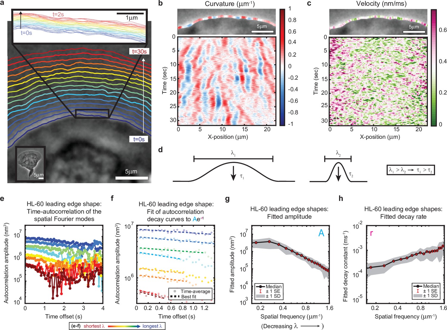
High-speed, high-resolution imaging reveals fine-scale fluctuations in leading edge shape.
(a–c) Example of leading edge fluctuations extracted from a representative migrating HL-60 cell. (a) Phase contrast microscopy image from the first frame of a movie, overlaid with segmented leading edge shapes from time points increasing from blue to red in 2 s intervals. Top Inset: Magnification of the segmented leading edge between t = 0–2 s increasing from blue to red in 50 ms intervals. Bottom Inset: A de-magnified image of the whole cell at the last time point. (b–c) Kymographs of curvature (b) and velocity (c). Note the velocity is always positive, so no part of the leading edge undergoes retraction. (d) Schematic demonstrating a commonly observed trend between fluctuation wavelength and relaxation time. (e) Autocorrelation amplitude (complex magnitude) of the spatial Fourier transform plotted as a function of time offset from a representative cell. Each line corresponds to a different spatial frequency in the range of 0.22–0.62 µm–1 (corresponding to a wavelength in the range of 4.5–1.6 µm) in 0.056 µm–1 intervals. (f) Best fit of the autocorrelation data shown in (e) to an exponential decay, fitted out to a drop in amplitude of 2/e. (g–h) Fitted parameters of the autocorrelation averaged over 67 cells. Data from this figure can be found in Figure 1—source data 1.
-
Figure 1—source data 1
Source data corresponding to plots in Figure 1.
See Readme for a description of the contents, and the locations of the corresponding plots in the figure.
- https://cdn.elifesciences.org/articles/74389/elife-74389-fig1-data1-v3.zip
Figure 1—figure supplement 1
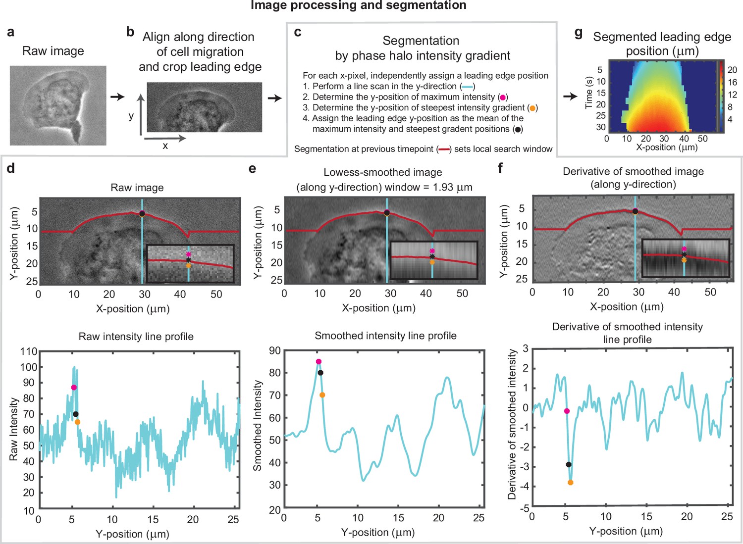
Overview of cell segmentation analysis pipeline.
Example of image processing and leading edge segmentation for a single cell. (a) Example raw image of a migrating cell. (b) Image of the same cell after aligning the image in the direction of motion of the cell and then cropping the leading edge. (c–f) Segmentation process shown for the example cell, for a single time point. (c) Steps for performing the segmentation, as well as a legend for (d-f). (d-f) Image of the cell (top) and a vertical line scan of the pixel intensity (blue line, bottom) for (d) the raw image, (e) the image smoothed along the vertical direction, and (f) the vertical derivative of the smoothed image. Super-imposed on each plot is the position of maximum intensity (pink dot), the position of steepest negative gradient (orange dot), and the mean of these two positions (black dot), which was used as the segmented leading edge point. The search for these maxima along each line scan was performed in a window around the segmented leading edge position at the previous time point (red line). (g) Kymograph of the segmented leading edge positions for all time points in the video.
Figure 1—figure supplement 2
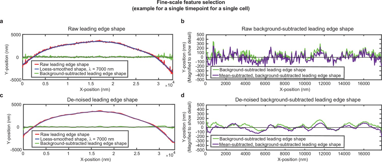
Overview of analysis pipeline to extract fine-scale leading edge shape features.
An example of the fine-scale feature selection process for the same cell shown in Figure 1—figure supplement 1. (a,c) Raw leading edge shape (red line), the Loess-smoothed shape (blue line), and the difference between the raw and smoothed shape (green line) for both (a) raw data and (c) de-noised data, to emphasize the ability of background-subtraction to capture fine-scale fluctuation events. (b,d) Green line: The same data as shown in (a,c), with the y-position magnified to show fine-scale shape features. Purple line: The same data after subtracting the time-averaged y-position for each x-position. This subtraction pulls out fluctuations around the average y-position for each x-position. The raw background-subtracted leading edge shapes (panel (b), purple curve) were used in subsequent analysis.
Figure 1—figure supplement 3
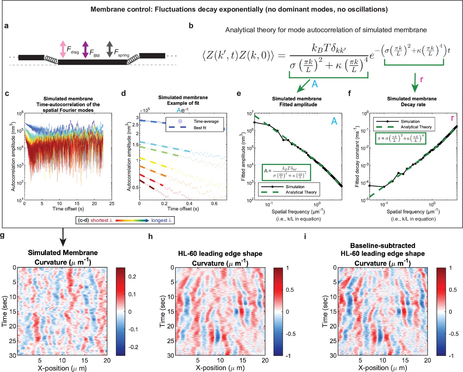
Control for analysis I.
Validation of spatial Fourier mode autocorrelation analysis using analytical theory for simulated membrane dynamics. (a–f) Simulated membrane control exhibiting exponentially decaying fluctuations. (a) Freely fluctuating membrane model schematic. Black lines, membrane; Physical parameters: Fspring, forces between membrane segments; FBM, Brownian forces; Fdrag, viscous drag. (b) Analytical theory for membrane freely fluctuating under Brownian motion: Autocorrelation amplitude <Z(k’,t)Z(k,0) > as a function of wavemode, k, and time, t, is an exponential decay function. Parameters include the Boltzmann constant kB, temperature T, elastic modulus σ, bending modulus κ, and membrane rest length L. (c) Autocorrelation amplitude (complex magnitude) of the spatial Fourier transform plotted as a function of time offset from a representative simulation. Each line corresponds to a different spatial frequency in the range of 0.2–0.55 µm–1 (corresponding to a wavelength in the range of 5.0–1.8 µm) in 0.05 µm–1 intervals. (d) Best fit of the autocorrelation data shown in (c) to an exponential decay, fitted out to a drop in amplitude of 2/e. (e–f) Fitted parameters for the same simulation shown in (c–d) showing good agreement with the analytical theory. (g–i) The most obvious features of the curvature kymograph (apparent dominant wavemodes and apparent oscillations) are misleading, and are recovered for a system with (by definition) no dominant or oscillatory modes. In the experimental data, these features are retained following baseline subtraction in the pre-processing step (see Figure 1—figure supplement 2). Curvature kymograph for (g) a simulated membrane, (h) the HL-60 leading edge displayed in Figure 1, and (i) the same HL-60 cell leading edge shown in (h) with curvature fitting performed after baseline-subtraction.
Figure 1—figure supplement 4
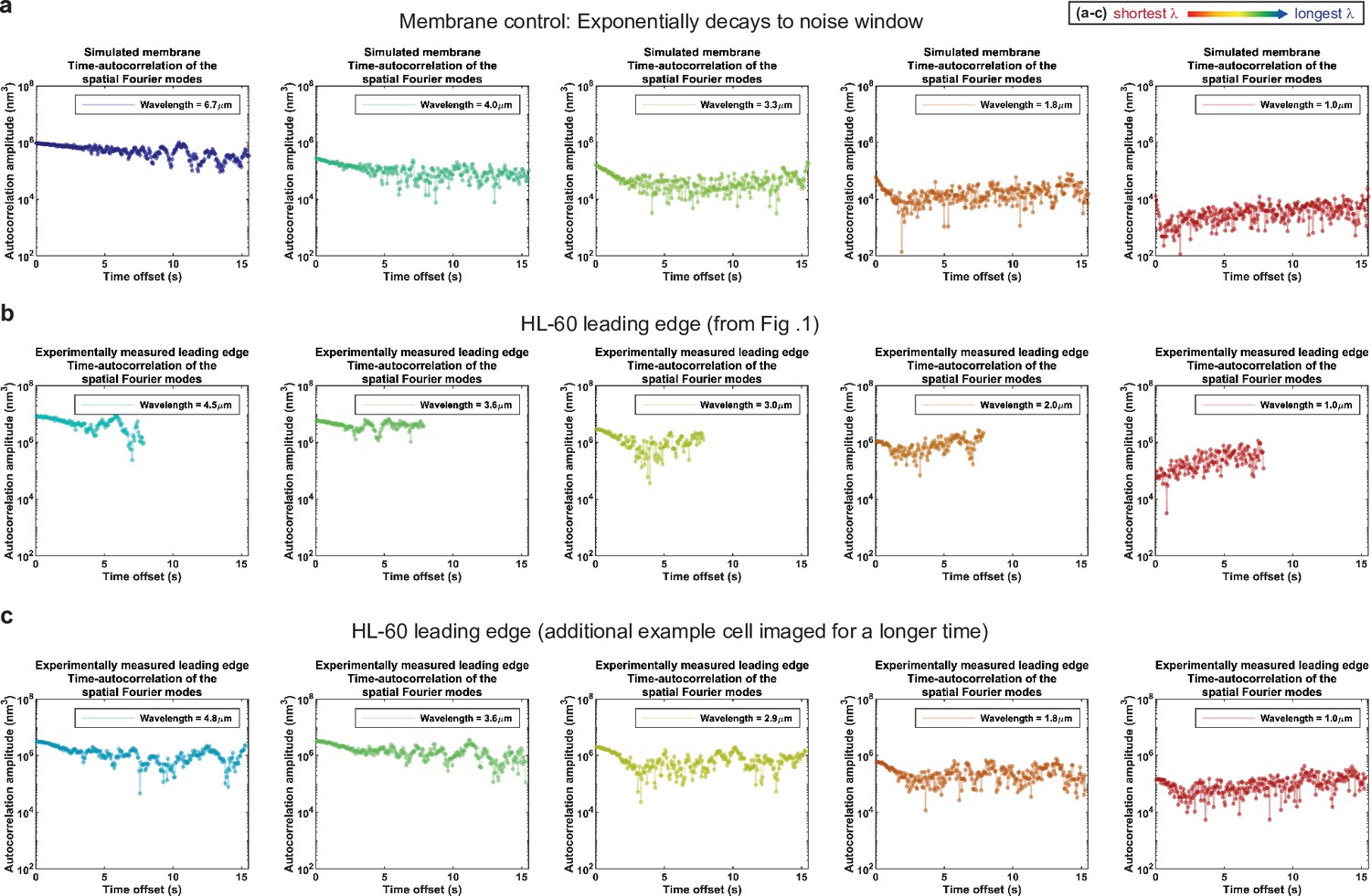
Control for analysis II.
Autocorrelation analysis of HL-60 leading edges shows exponential decay to a noise window at long times. (a–c) Autocorrelation amplitude (complex magnitude) of the spatial Fourier transform plotted as a function of time offset from (a) the simulated membrane control from Figure 1—figure supplement 3, (b) the HL-60 leading edge displayed in Figure 1, and (c) a different HL-60 cell leading edge that was imaged for longer time. Each panel shows the autocorrelation results for a different wavelength, where the color represents the wavelength.
Figure 1—figure supplement 5
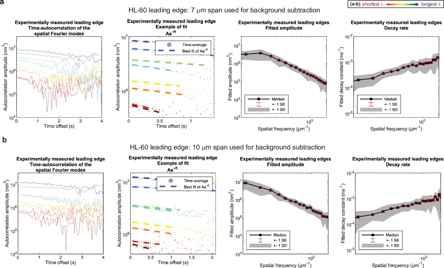
Control for analysis III.
No new features emerge upon a ~50% increase in span used for background subtraction. (a–b) Autocorrelation analysis results on HL-60 cell leading edges as shown in Figure 1, using either (a) a 7 μm span or (b) a 10 μm span to perform background subtraction on the leading edge shape during pre-processing. (A typical cell is ~15–20 μm wide.).
Figure 1—figure supplement 6
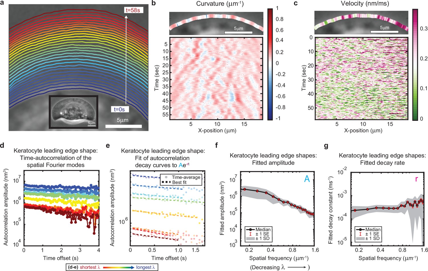
Leading edge fluctuation behavior is reproduced in fish epidermal keratocytes.
(a–c) Example of leading edge fluctuations extracted from a representative migrating fish epidermal keratocyte, plotted as in Figure 1a–c. Note differences in scale for time, x-position, and velocity from the equivalent plots in Figure 1. Segmented leading edges in (a) are still plotted in 2 s time intervals. (d) Autocorrelation amplitude (complex magnitude) of the spatial Fourier transform plotted as a function of time offset from a representative cell, plotted as in Figure 1e. Each line corresponds to a different spatial frequency in the range of 0.19–0.52 µm–1 (corresponding to a wavelength in the range of 5.3–1.9 µm) in 0.047 µm–1 intervals. (e) Best fit of the autocorrelation data shown in (d) to an exponential decay, plotted as in Figure 1f. Note differences in scale for time offset and autocorrelation amplitude from the equivalent plot in Figure 1. (f–g) Fitted parameters of the autocorrelation averaged over 16 videos of 12 cells, plotted as in Figure 1g–h.
Figure 2 with 3 supplements
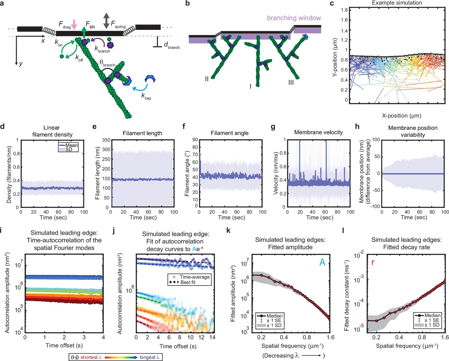
Minimal model of branched actin growth recapitulates leading edge stability and shape fluctuation relaxation.
(a–b) Model schematic. Black lines, membrane; green circles, actin; purple flowers, Arp2/3 complex; blue crescents, capping protein. Rates: kon, polymerization; koff, depolymerization; kbranch, branching; kcap, capping. θbranch, branching angle. dbranch, branching window. Physical parameters: Fspring, forces between membrane segments; FBR, force of filaments on the membrane (Brownian ratchet); Fdrag, viscous drag. (b) Schematic demonstrating filament angle evolution. Filaments growing perpendicular to the leading edge (I) outcompete their progeny (branches), leading to a reduction in filament density; filaments growing at an angle (II and III) make successful progeny. Filaments spreading down a membrane positional gradient (II) are more evolutionarily successful than those spreading up (III). (c) Simulation snapshot: Black lines, membrane; colored lines, filament equilibrium position and shape; gray dots, barbed ends; black dots, capped ends; filament color, x-position of membrane segment filament is pushing (increasing across the x-axis from blue to red). (d-h) For a representative simulation, mean (solid line) and standard deviation (shading) of various membrane and actin filament properties as a function of simulation time. Note for linear filament density (d) lamellipodia are ~10 filament stacks tall along the z-axis, giving mean filament spacing of 10/density, or ~30 nm. (i–l) Autocorrelation analysis and fitting for a representative simulation (i–j) as well as best fit parameters averaged over 40 simulations (k–l). Data from this figure can be found in Figure 2—source data 1.
-
Figure 2—source data 1
Source data corresponding to plots in Figure 2.
See Readme for a description of the contents, and the locations of the corresponding plots in the figure.
- https://cdn.elifesciences.org/articles/74389/elife-74389-fig2-data1-v3.zip
Figure 2—figure supplement 1
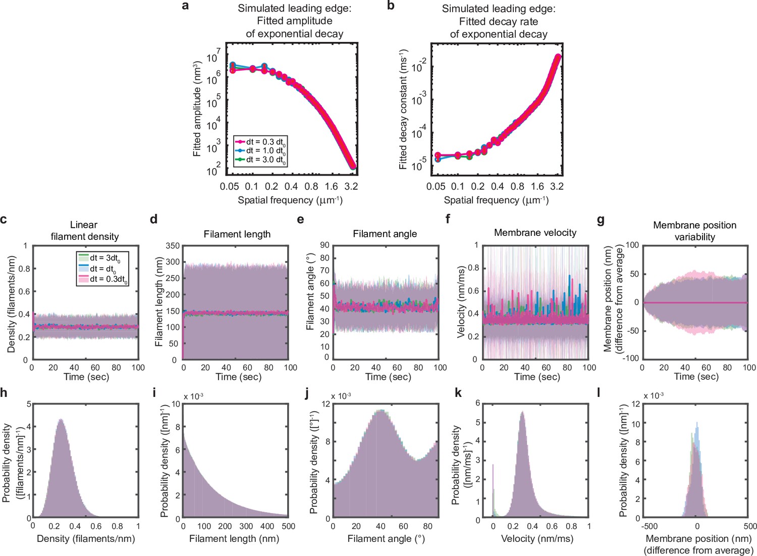
Simulations are performed at sufficient temporal discretization.
A summary of leading edge fluctuations and actin network properties for simulations using the standard timestep (blue), a timestep three-fold larger (green), and a timestep three times smaller (pink). Increasing the temporal discretization (decreasing the timestep) did not affect the simulation results, suggesting this chosen timestep is appropriate to resolve the fastest timescales in the system. (a–b) Fitted leading edge fluctuation parameters plotted as in Figure 5f–g. (c–g) Actin network properties plotted as in Figure 2d–h. (h–l) Histograms of actin network property distributions at steady state (last 90 s of the simulated timepoints in panels c-g). The y-axis corresponds to the probability density per histogram bin width. The sum of the probability density across all bins is equal to one. Histograms with bin widths less than one may have a probability density greater than one.
Figure 2—figure supplement 2
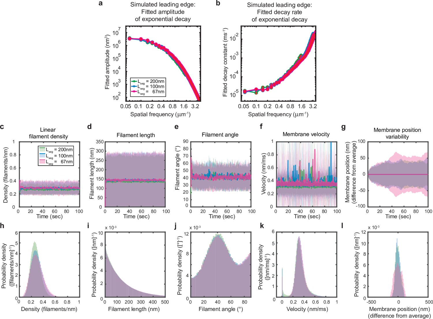
Simulations are performed at sufficient spatial discretization.
(a–l) A summary of leading edge fluctuations and actin network properties, plotted as in Figure 2—figure supplement 1, for simulations using the standard membrane segment length (blue), a segment size twofold larger (green) and a length 30% smaller (pink). Increasing the spatial discretization (decreasing the segment size) did not significantly change the leading edge properties, suggesting the chosen discretization is sufficient to approximate a continuous membrane.
Figure 2—figure supplement 3
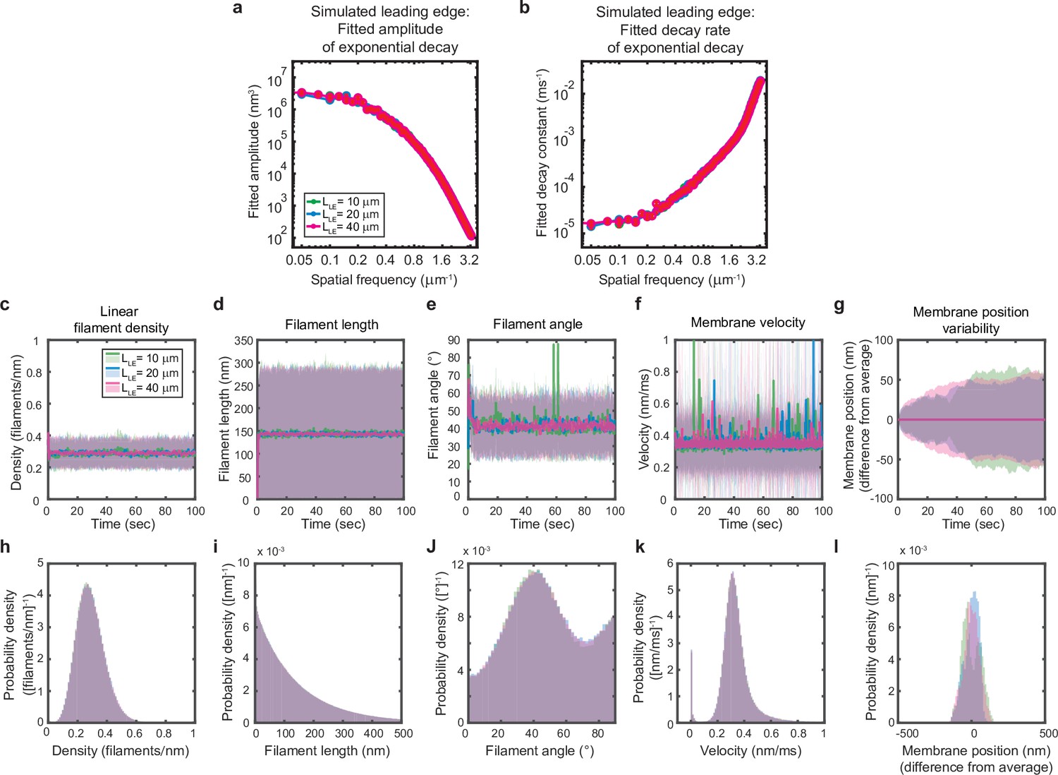
Simulated leading edge behavior is not affected by leading edge length.
(a–l) A summary of leading edge fluctuations and actin network properties, plotted as in Figure 2—figure supplement 1, for simulations using the standard leading edge length (blue), a length two times smaller (green) and a length twofold larger (pink). Increasing the leading edge length did not change the properties of the fluctuations and actin network.
Figure 3
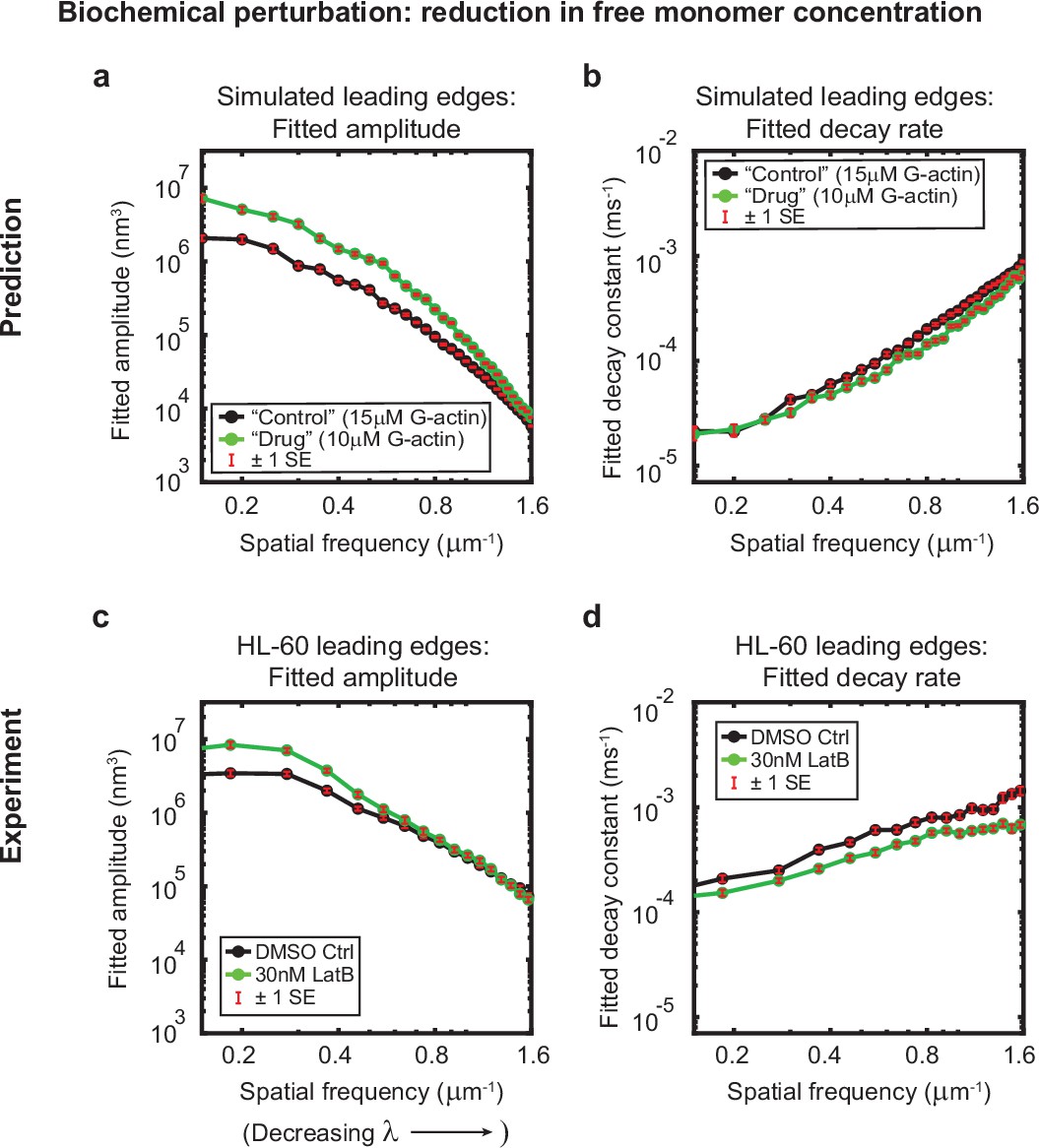
Minimal model correctly predicts response of HL-60 cells to drug treatment.
Predicted and experimentally-measured response of the autocorrelation decay fit parameters to drug treatment with Latrunculin B, plotted as in Figure 1g–h. (a–b) Predicted response to a reduction in the free monomer concentration (green, 10 µM G-actin) compared to the standard concentration used in this work (black, 15 µM G-actin) – medians over 40 simulations for each condition. (c–d) Experimentally measured behavior: DMSO control – medians over 67 cells (same data as plotted in Figure 1g–h). 30 nM Latrunculin B – medians over 34 cells. Data from this figure can be found in Figure 3—source data 1.
-
Figure 3—source data 1
Source data corresponding to plots in Figure 3.
See Readme for a description of the contents, and the locations of the corresponding plots in the figure.
- https://cdn.elifesciences.org/articles/74389/elife-74389-fig3-data1-v3.zip
Figure 4
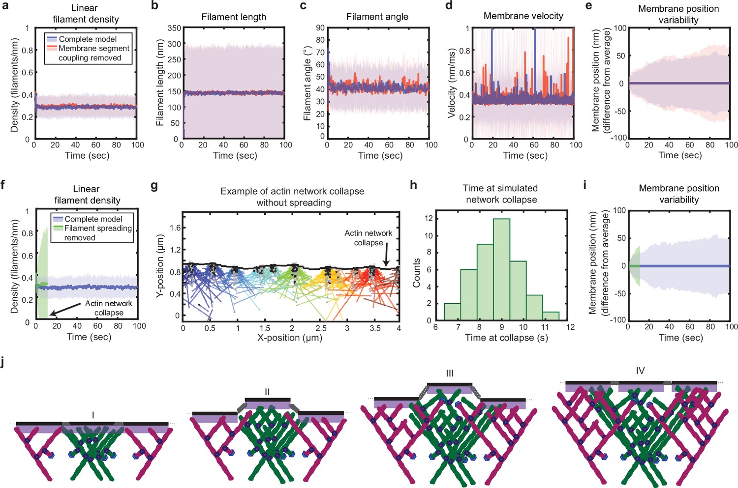
Simulated lamellipodial stability is governed by leading edge geometry.
(a–e) Comparison of leading edge properties with and without the coupling of the membrane segments by tension and bending rigidity (no coupling: Fspring = 0 in Figure 2a), plotted as in Figure 2d–h. (f–i) Comparison of leading edge properties with and without the ability of filaments to spread between neighboring membrane segments. (g) A snapshot of the simulation after filament network collapse (defined as a state where at least 25% of the membrane segments have no associated filaments). (f,g,i) Plots made from the same simulation. (h) A histogram of the average time to network collapse over 40 simulations. (j) Schematic representing the proposed molecular mechanism underlying the stability of leading edge shape, with time increasing from I-IV. Data from this figure can be found in Figure 4—source data 1.
-
Figure 4—source data 1
Source data corresponding to plots in Figure 4.
See Readme for a description of the contents, and the locations of the corresponding plots in the figure.
- https://cdn.elifesciences.org/articles/74389/elife-74389-fig4-data1-v3.zip
Figure 5
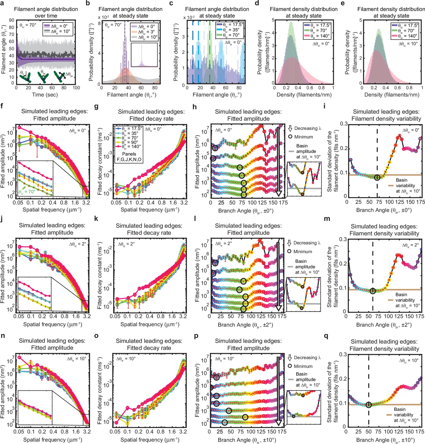
The genetically-encoded Arp2/3-mediated branching angle is optimal for suppressing leading edge fluctuations.
(a–c) Time course (a) and steady state distribution (b–c) of the filament angle (θf) for simulations with various branching angle standard deviations (Δθbr), (a–b) and means (θbr), (c). Dashed lines represent θbr/2 plus integer multiples of θbr. (d–e) Steady state filament density distribution as a function of the mean branching angle in the context of Δθbr=0° (d) and Δθbr=10° (e). (a–b, d–e) Results from a representative simulation for each condition. (c) Data integrated over 40 simulations. (f–q) Predicted response of leading edge fluctuations and filament density variability to changes in the branch angle and branch angle variability, medians over 40 simulations for each condition. Red error bars – standard error. Color map is identical for panels c-q. (h,l,p) Fitted amplitude as a function of branch angle, where each line represents a different spatial frequency, increasing from 0.2 to 3.2 µm–1 in intervals of 0.5 µm–1. Insets have identical x-axes to main panels. (i,m,q) Standard deviation of the filament density at steady state plotted as a function of branch angle. Note the x- and y-axes limits in (f–g, j–k, n–o) are expanded compared to the equivalent panels in Figures 1—3. Data from this figure can be found in Figure 5—source data 1.
-
Figure 5—source data 1
Source data corresponding to plots in Figure 5.
See Readme for a description of the contents, and the locations of the corresponding plots in the figure.
- https://cdn.elifesciences.org/articles/74389/elife-74389-fig5-data1-v3.zip
Videos
Video 1
Segmentation overlaid onto migrating HL-60 cell.
Time lapse video representation of segmentation results shown in Figure 1a.
Video 2
Example fish epidermal keratocyte.
Time lapse video corresponding to the data shown in Figure 1—figure supplement 6a-e.
Video 3
Example simulation.
Time lapse video representation of simulation results shown in Figure 2c.
Video 4
Example HL-60 cell treated with 30 nM latrunculin B.
Video 5
Example HL-60 cell treated with 0.1% DMSO vehicle control.
Video 6
Example HL-60 cell treated with 100 μM CK-666.
Tables
Table 1
Actin network growth parameters.
Parameters listed are the default used for the simulations.
| Notation | Meaning | Value | Source |
|---|---|---|---|
| M | Free monomer concentration | 15 µM | Cooper, 1991; Marchand et al., 1995 |
| kon | Polymerization rate | 11∙10–3 monomers ms–1 µM–1 | Pollard, 1986 |
| koff | Depolymerization rate | 10–3 monomers ms–1 | Pollard, 1986 |
| kcap | Capping rate | 3∙10–3 ms–1 | ~3∙10–3 µM–1 ms-1 Schafer et al., 1996at 1 µM capping protein Pollard et al., 2000 |
| kbranch | Branching rate | 4.5∙10–5 branches ms–1 µM–1 nm–1 | 50 nm branch spacing Svitkina et al., 1997; Svitkina and Borisy, 1999;Branch rate approximated such that elongation rate / branch rate = 50 nm; kbranch = (kon∙M∙lm)/(50 nm∙M∙ybranch) |
| ybranch | Branching window length | 15 nm | ~3–5 protein diameters away from the membrane |
| θbranch | Branching angle | 70 ± 10° | Mullins et al., 1998; Volkmann et al., 2001; Rouiller et al., 2008; Blanchoin et al., 2000; Cai et al., 2008; Svitkina and Borisy, 1999 |
| lp | Actin filament persistence length | 1 µm | Käs et al., 1996 |
| lm | Actin monomer length | 2.7 nm | Pollard, 1986 |
Table 2
Physical parameters.
Parameters listed are the default used for the simulations.
| Notation | Meaning | Value | Source |
|---|---|---|---|
| kB | Boltzmann constant | 0.0183 pN nm K–1 | – |
| T | Temperature | 310.15 K | – |
| σ | Membrane tension | 0.03 pN nm–1 | Lieber et al., 2013 |
| κ | Membrane bending modulus | 140 pN nm | Lieber et al., 2013 |
| ηw | Viscosity of water at 37 °C | 7∙10–7 pN ns nm–2 | – |
| η | Effective viscosity at the leading edge | 3000 ηw | ~ effective viscosity of micron-scale beads in cytoplasm Wirtz, 2009 |
| L | Leading edge length | 20 µm | This work |
| h | Leading edge height | 200 nm | Abraham et al., 1999; Laurent et al., 2005; Urban et al., 2010 |
| Δx | Membrane segment length | 100 nm | – |
| N | Number of membrane segments | 200 | – |
Additional files
Download links
A two-part list of links to download the article, or parts of the article, in various formats.
Downloads (link to download the article as PDF)
Open citations (links to open the citations from this article in various online reference manager services)
Cite this article (links to download the citations from this article in formats compatible with various reference manager tools)
Leading edge maintenance in migrating cells is an emergent property of branched actin network growth
eLife 11:e74389.
https://doi.org/10.7554/eLife.74389


