Competition for fluctuating resources reproduces statistics of species abundance over time across wide-ranging microbiotas
- Department of Bioengineering, Stanford University, United States
- Department of Applied Physics, Stanford University, United States
- Chan Zuckerberg Biohub, United States
- Department of Microbiology and Immunology, Stanford University School of Medicine, United States
Figures
Figure 1 with 2 supplements
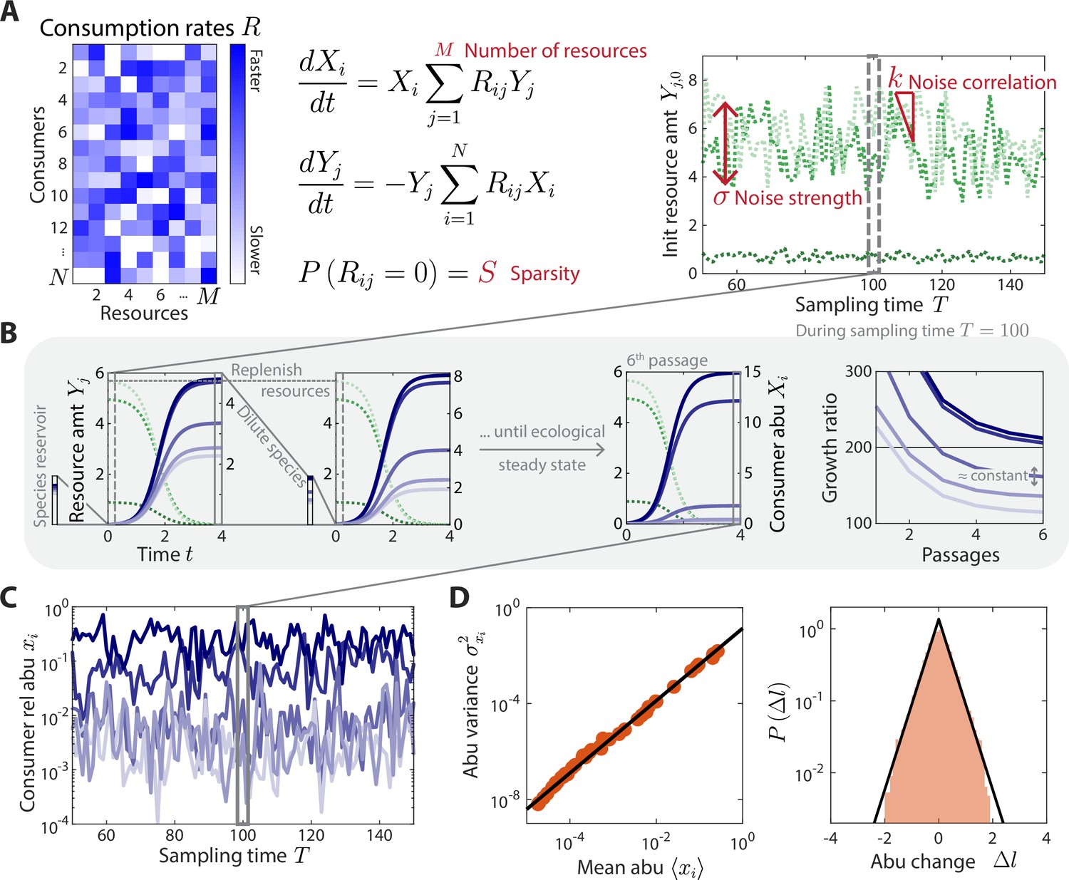
A coarse-grained consumer-resource model with fluctuating resource amounts.
(A) In the consumer-resource model, denotes the abundance (abu) of consumer i and denotes the amount of coarse-grained resource . The dynamics of the model are specified by consumption rates for consumers and resources. is drawn from a uniform distribution, and each is set to zero with probability , the sparsity of resource competition. The initial resource amount at each sampling time fluctuates with noise strength and restoring force . is estimated from each data set, and the four free ensemble level parameters are highlighted in red. (B) Shown are the dynamics of the model within one sampling time (, dashed gray box) for a subset of consumers and resources in a typical simulation. At each sampling time , the model was simulated under a serial dilution scheme in which consumers (solid blue lines) grew until all resources (dotted green lines) were depleted, after which all consumer abundances were diluted by a fixed factor and resource amounts were replenished to . Each sampling time was initiated from an external reservoir of consumers, with all consumers present at equal abundance. Dilutions were repeated until an approximate ecological steady state was reached in which the ratios of final to initial abundances of all consumers changed by less than 5% of between subsequent dilutions (Materials and methods). The relative abundances at sampling time were obtained from the final species abundances at steady state. (C) The model maps a set of fluctuating resource amounts to a time series of consumer relative abundances that can be compared to experimental measurements. (D) The simulated time series in (C) exhibits statistical behaviors that reproduce those found in experiments, including a power law scaling between the abundance variance and mean over time of each species (left) and an approximately exponential distribution of abundance changes (right). Black lines denote the best linear fit (left) and the best fit exponential distribution (right). The simulation shown in (A–D) was generated with .
Figure 1—figure supplement 1
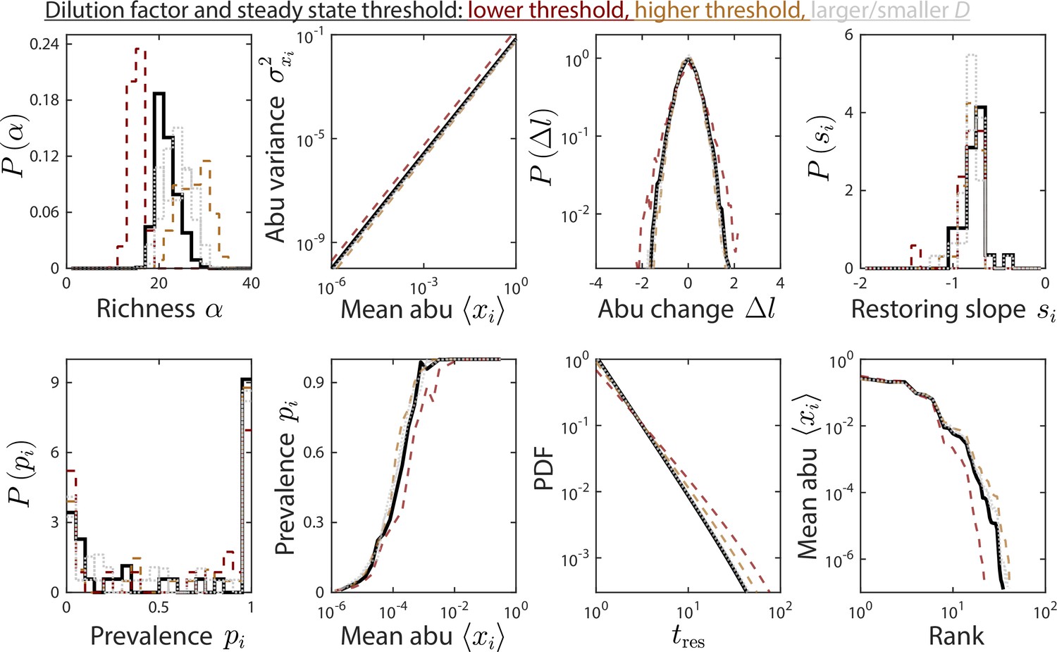
The dilution factor and steady-state threshold do not substantially affect time series statistics.
Depicted are time series statistics of relative abundances (abu) for one instance of the parameter set used in Figures 1 and 2, simulated using a dilution factor and a steady-state threshold of 5% (solid black line), or with a threshold of 5% (dotted gray lines), and a threshold of 1% and 10% with (dashed brown and orange lines, respectively).
Figure 1—figure supplement 2
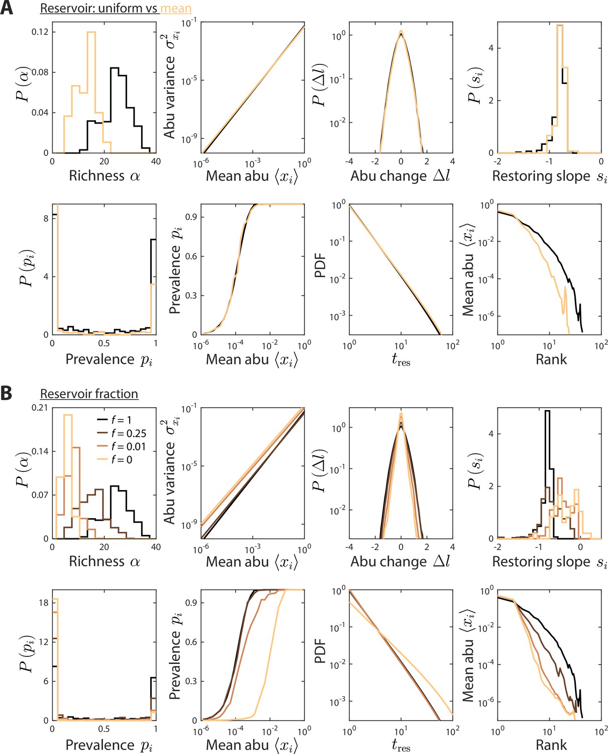
Reservoir composition does not substantially affect time series statistics.
(A) Depicted are model predictions using the parameter set in Figures 1 and 2, with two definitions of the reservoir of consumers used to initialize the dynamics at each sampling time: a uniform reservoir in which all consumers are present at equal abundance (black), and a mean reservoir equal to the steady-state composition given by the set point environment initialized with a uniform reservoir (light brown). Most statistics were not substantially affected. The richness was lower when initializing with the mean reservoir, but the susceptibility of richness to model parameters is expected to remain qualitatively the same. (B) Depicted are model predictions with varying reservoir fraction , in which initial consumer abundances (abu) during sampling time were determined by a combination of the reservoir and the steady state at the previous sampling time, . Many statistics were substantially affected by the value of . Notably, the contribution from the previous steady state introduces autocorrelations, thereby increasing the mean restoring slope. Moreover, the absence of a reservoir substantially decreased richness since low abundance consumers do not have enough time to grow to high abundances even when resource levels fluctuate in their favor.
Figure 2 with 2 supplements

A coarse-grained consumer-resource model with fluctuating resource amounts reproduces experimentally observed statistics in an abundance time series from daily sampling of a human gut microbiota.
In all panels, blue points and bars denote experimental data analyzed and aggregated at the family level (Caporaso et al., 2011). Red lines and shading denote best fit model predictions as the mean and standard deviation, respectively, across 20 random instances of the best fit ensemble level parameters, . (A–D) Illustrations of various time series statistics in (E–L). (A) The distribution of richness , the number of consumers present at a sampling time, and its mean are well fit by the model. (B) The variance and mean over time of each family’s abundance (abu) scale as a power law with exponent . Here, in experimental data and in simulations. (C) The distribution of log10(abundance change) across all families is well fit by an exponential with standard deviation . The gray line denotes the best fit exponential distribution, and is largely overlapping with the model prediction in red. (D) The distribution of restoring slopes , defined based on the linear regression between the abundance change and the relative abundance for a species across time, is tightly distributed around a mean that reflects the environmental restoring force. Best fit values of model parameters were determined by minimizing errors in , , , and (E–H, respectively). Using these values, our model also reproduced the distribution of prevalences (fraction of sampling times in which a consumer is present, I), the relationship between prevalence and mean abundance (J), the distributions of residence and return times (durations of sustained presence or absence, respectively, as illustrated in D) (K), and the rank distribution of abundances (L).
Figure 2—figure supplement 1

Grouping at a coarser taxonomic level results in similar time series statistics.
Shown are data from Caporaso et al., 2011, as in Figure 2, but with relative abundances (abu) grouped and analyzed at the class instead of family level. The best fit model predictions are shown, with best fit parameters .
Figure 2—figure supplement 2
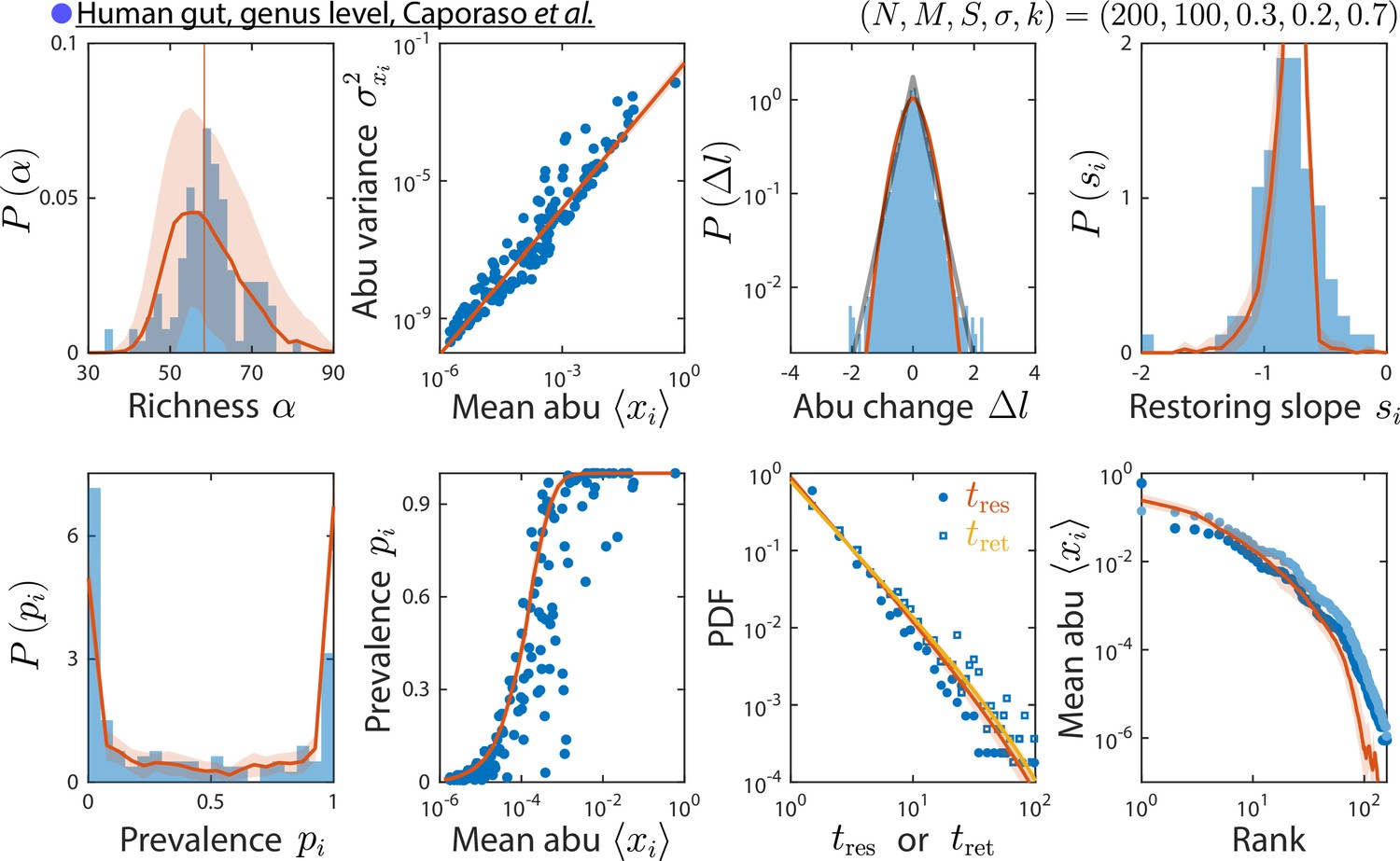
The consumer-resource (CR) model can reproduce time series statistics at the genus level of a human gut microbiota.
Shown are data from Caporaso et al., 2011, as in Figure 2, but with relative abundances (abu) grouped and analyzed at the genus level. Data are compared against the CR model with the best fit parameters shown. The rank distribution of mean abundances shown in light blue was obtained after removing the dominant Bacteroides genus and recomputing relative abundances.
Figure 3 with 5 supplements
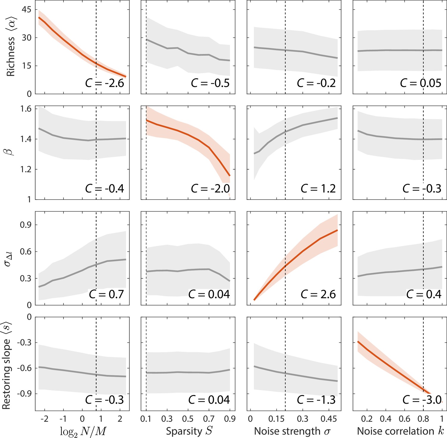
Macroscopic parameters of resource competition affect time series statistics in distinct manners.
Shown are the changes in time series statistics (y-axis) in response to changes in model parameters (x-axis) for a comprehensive search across relevant regions of parameter space. Lines and shading show the mean and standard deviation of a statistic at the given parameter value across variations in all other parameters. Data are plotted in red when the corresponding susceptibility , indicating that statistic is strongly affected by parameter regardless of the values of other parameters. Dashed lines highlight best fit parameter values to the experimental data in Figure 2. Simulations were carried out for across , in 0.1 increments, in 0.05 increments, and in 0.1 increments.
Figure 3—figure supplement 1

Time series statistics are differentially susceptible to model parameters.
Twenty-eight relative abundance (abu) time series statistics were clustered (A) and ranked (B) according to their susceptibilities to identify statistics that strongly constrain the values of key parameters.
Figure 3—figure supplement 2
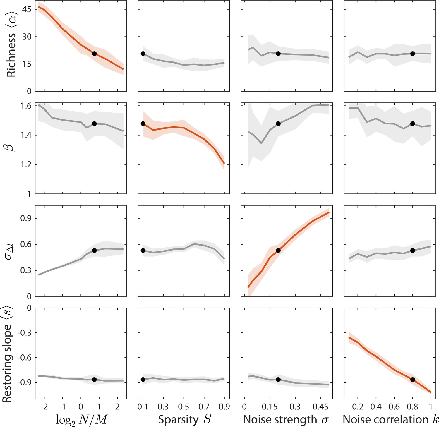
Local susceptibilities behave similarly to their global counterparts.
Shown are changes in time series statistics (y-axis) in response to changes in model parameters (x-axis) as in Figure 3. Here, lines and shading show the mean and standard deviation of a statistic at the given parameter value with other parameters fixed to their best fit values, as opposed to Figure 3 in which other parameters were averaged across their entire ranges. Black dots denote the best fit values.
Figure 3—figure supplement 3
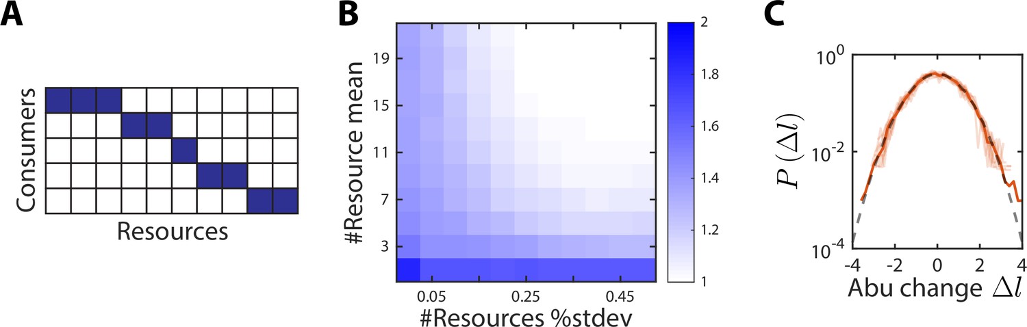
A no-competition model provides a partial explanation for the scaling exponent between and .
(A) In the no-competition model, each consumer consumes a disjoint set of resources. (B) The mean and standard deviation of the number of resources consumed per consumer determine the scaling exponent . Shown is the average value of over 1000 random instances of the no-competition model, across values of the mean number of resources consumed per consumer (y-axis) and the standard deviation in the number of resources consumed divided by the mean (x-axis). In this example, the model involved 10 consumers. At large mean number of resources consumed and high variance (top right), , whereas when each consumer utilizes its own unique resource (bottom left), . (C) Aggregate (solid orange line) and individual (light orange lines) distributions of abundance (abu) changes are normal (gray dashed line) in the no-competition model. The distributions of abundance changes, normalized by their sample standard deviations, are shown for an example simulation with 7 ± 1 resources per consumer.
Figure 3—figure supplement 4

Sparsity and the number of metabolites determine the shape of the distribution of abundance changes .
(A) Shown is the average goodness of fit (GOF, as determined by the p-value of the Kolmogorov-Smirnov test) of to an exponential (left) or a normal (right) distribution, for the distribution aggregated over all consumers (top) or the median value across the distributions of individual consumers (bottom). Larger values (blue) denote better fits. Green letters denote examples shown in (B). The other model parameters were fixed at as in Figure 2. (B) Shown are two regimes that result in an exponential distribution of abundance (abu) changes. Example (a) demonstrates that when , the aggregated distribution is better fit by an exponential (black dotted line) than by a normal distribution (top), and that the median of the individual distributions is also better fit by an exponential (bottom). Example (b) demonstrates that when and is high, the aggregated distribution is still better fit by an exponential, but the median of the individual distributions is better fit by a normal distribution.
Figure 3—figure supplement 5
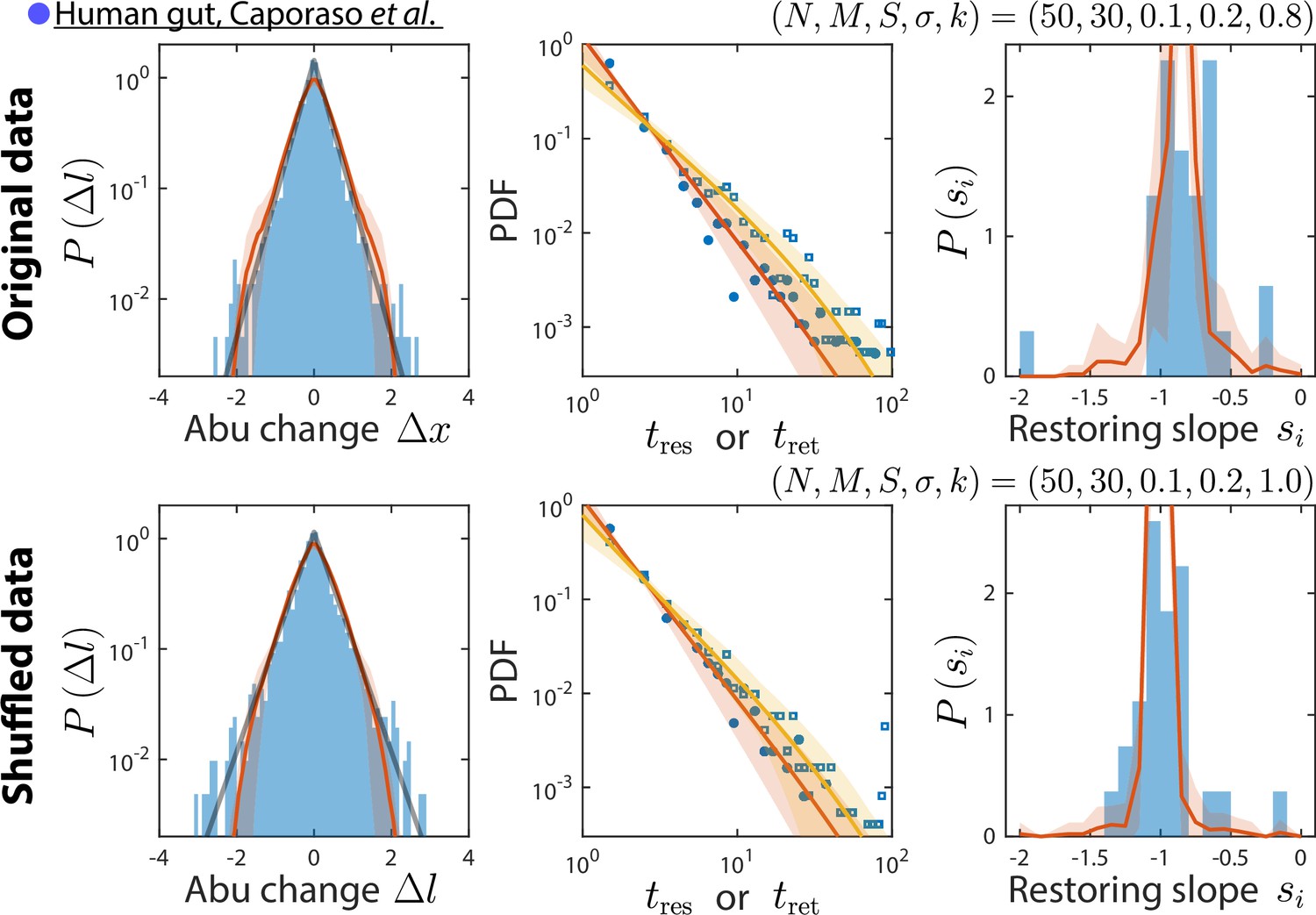
Our consumer-resource (CR) model is consistent with results obtained by shuffling time labels.
Shown are the original data from Caporaso et al., 2011, and the best fit model predictions as in Figure 2 (top), and the same data but with time labels shuffled (bottom). Only time series statistics that are affected by shuffling time labels are shown. Model predictions are based on the best fit parameters for the shuffled data, which were the same as for the original data except . Shuffling led to more negative restoring slopes, as expected from abolishing correlation between sampling times. The resulting mean restoring slope yielded a best fit value of , which in turn predicted the distributions of residence and return times after shuffling.
Figure 4 with 5 supplements
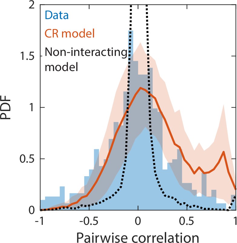
Correlations between abundances of consumer pairs were captured by the consumer-resource model, but not by a null model without interspecies interactions.
Shown in blue is the probability density function (PDF) of correlations between the abundances across sampling times of all consumer pairs for the experimental data in Figure 2. Red line represents parameter-free model predictions as in Figure 2, using the same best fit parameters; shading represents 1 standard deviation. Black dashed line shows predictions of a null model without interspecies interactions in which consumer abundances were drawn from independent normal distributions whose mean and variance were extracted from data.
Figure 4—figure supplement 1
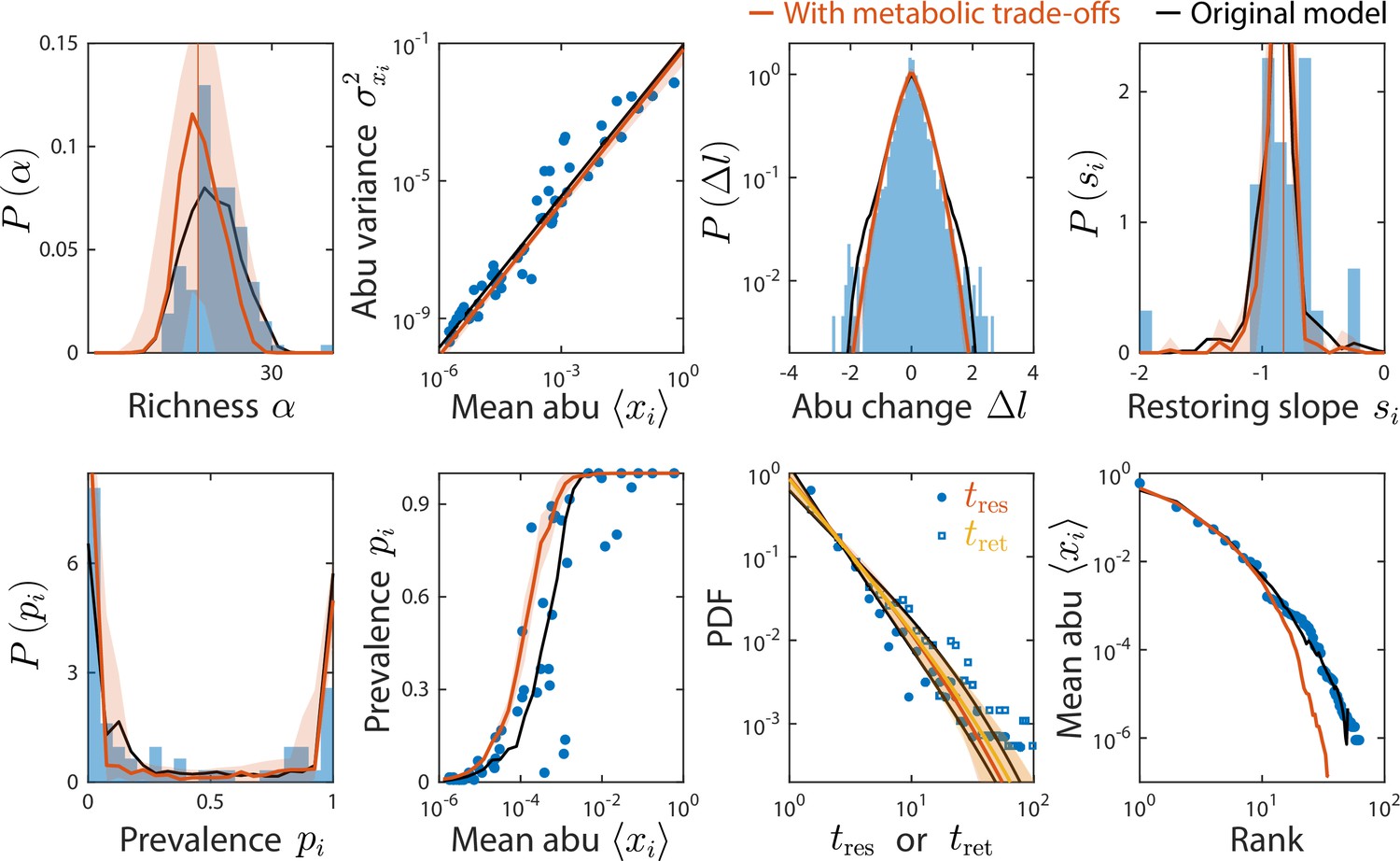
The consumer-resource (CR) model with metabolic trade-offs produces similar statistics as the original model and can also recapitulate experimental data.
Shown are data from Caporaso et al., 2011, as in Figure 2, with the mean prediction of the original CR model shown in black. Red (and yellow for ) lines and error regions denote predictions of the model including metabolic trade-offs (Materials and methods).
Figure 4—figure supplement 2
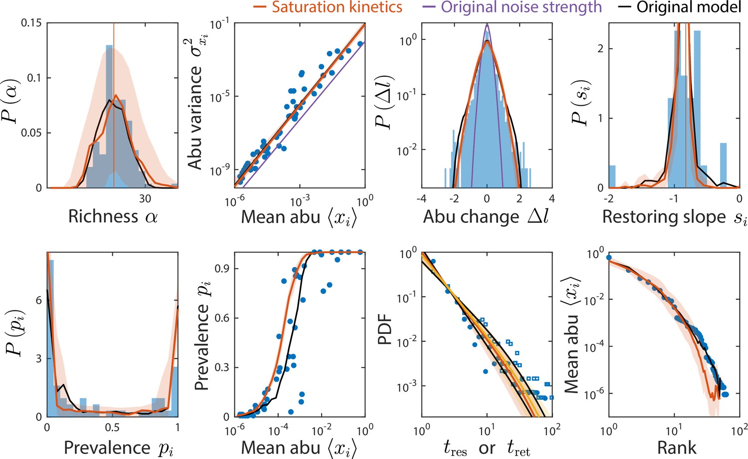
Consumer-resource (CR) model with saturation kinetics exhibits dampened fluctuations but can still reproduce experimentally observed statistics.
Shown are data from Caporaso et al., 2011, as in Figure 2, with predictions of the CR model with and without saturation kinetics (Materials and methods). Red (and yellow for ) lines denote the model with increased noise strength of , compared to purple, which denotes the model with saturation kinetics and the original noise strength . Predictions of the original CR model are shown in black. To aid visualization, only predictions from the model with the original noise strength that are visually different from the model with increased noise are shown.
Figure 4—figure supplement 3
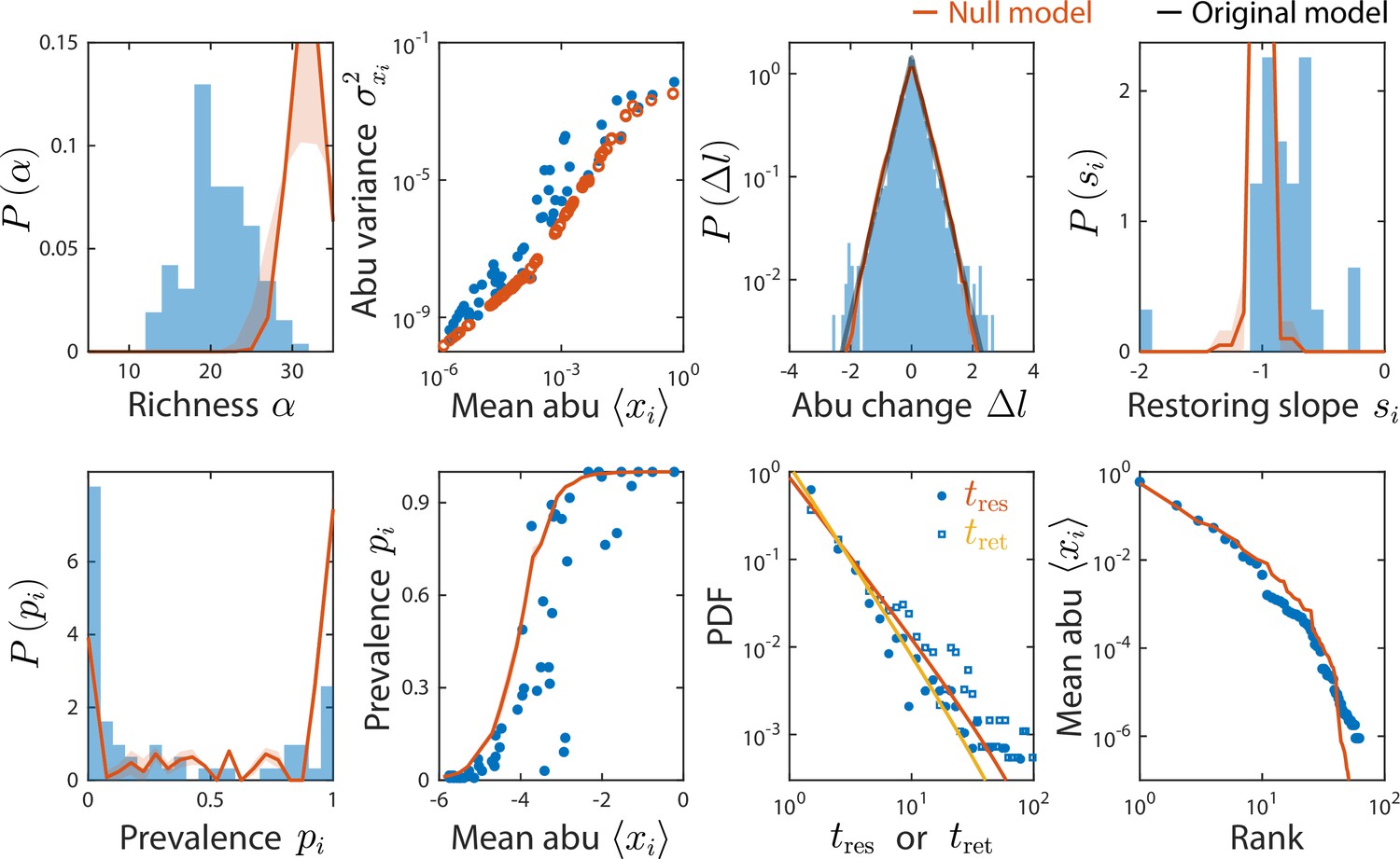
A non-interacting null model reproduced some, but not all, time series statistics.
Shown are data from Caporaso et al., 2011, as in Figure 2 and comparisons to a non-interacting null model in which consumer abundances were drawn from independent normal distributions whose mean and variance were extracted from data. As a result of its many free parameters, the null model was able to reproduce statistics such as the rank distribution of abundances, but was unable to reproduce the distributions of richness and residence and return times, nor the distribution of pairwise correlations (Figure 4).
Figure 4—figure supplement 4
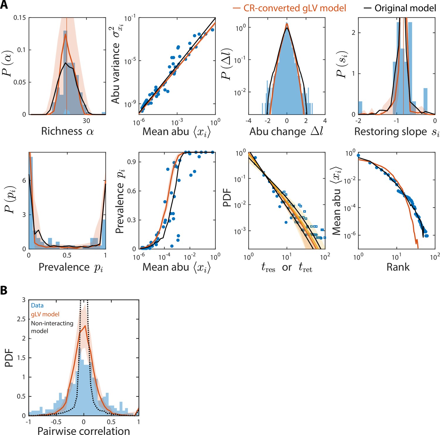
Generalized Lotka-Volterra (gLV) model with consumer-resource (CR)-converted interaction coefficients generates time series statistics similar to the original CR model and also recapitulates experimental data.
Shown are data from Caporaso et al., 2011, as in Figure 2, with predictions of the CR-converted gLV model (Materials and methods) for the time series statistics (A) and the distribution of pairwise correlations (B). Black denotes predictions of the original CR model (A) or the null model as in Figure 4—figure supplement 3 (B).
Figure 4—figure supplement 5
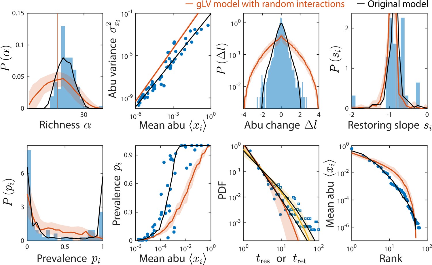
Generalized Lotka-Volterra (gLV) model with normally distributed interaction coefficients cannot reproduce experimental data.
Shown are data from Caporaso et al., 2011, as in Figure 2, with predictions of the gLV model with random interaction coefficients (Materials and methods). Predictions of the original consumer-resource (CR) model are shown in black.
Figure 5 with 6 supplements
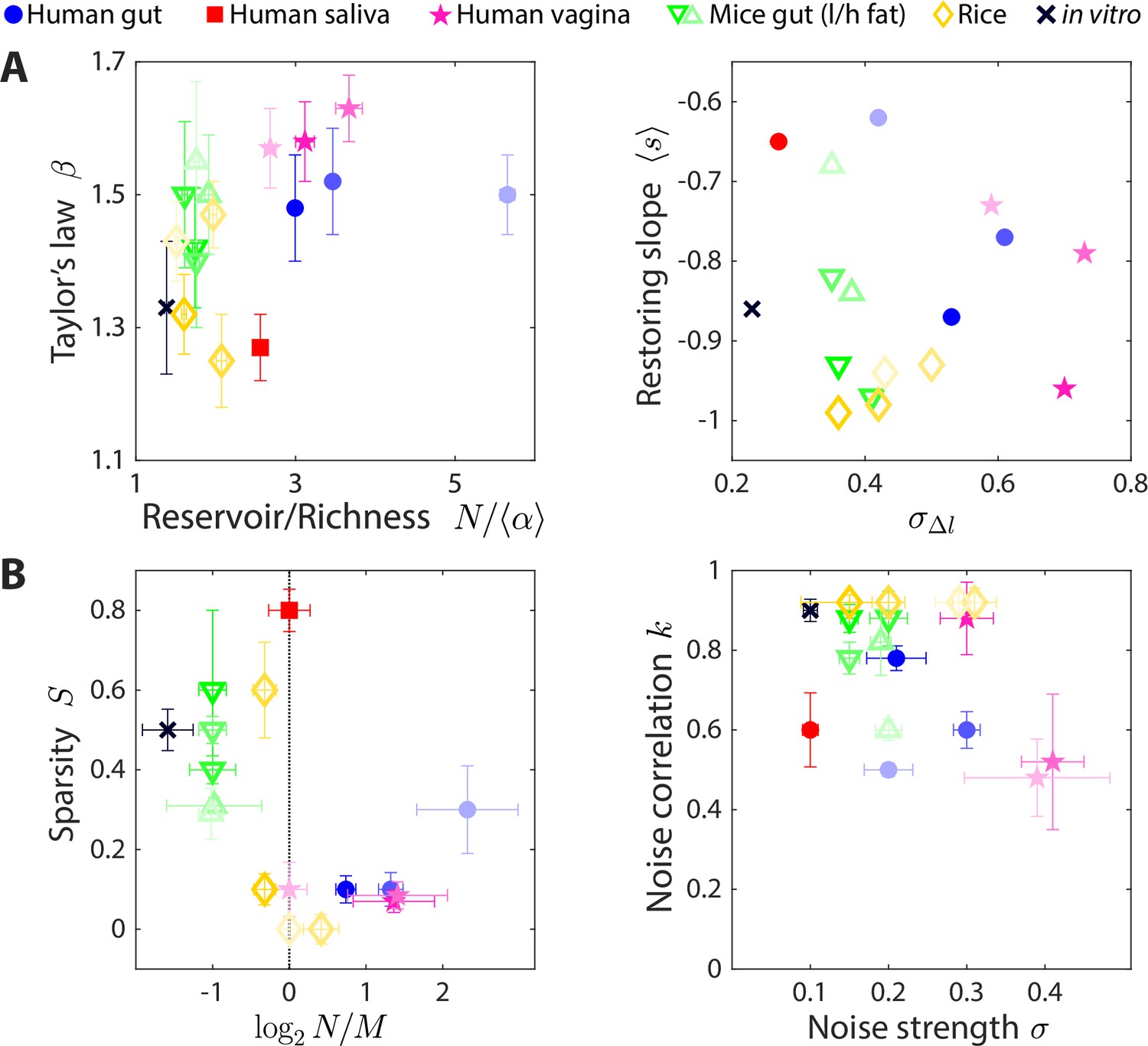
The statistics of wide-ranging microbiotas were captured by the coarse-grained consumer-resource model in different regimes of resource competition and environmental fluctuations.
Shown are time series statistics (A) and corresponding best fit model parameters (B) for human microbiotas from stool (Caporaso et al., 2011; David et al., 2014) (blue circles), saliva (David et al., 2014) (red square), and the vagina (Song et al., 2020) (pink stars), gut microbiotas of mice under low fat (green downward triangles) and high fat (green upward triangles) diets (Carmody et al., 2015), and plant microbiotas from the rice endosphere, rhizosphere, rhizoplane, and bulk soil (Edwards et al., 2018) (diamonds). (A) Microbiota origin generally dictates the scaling exponent and the ratio between the reservoir size N (number of observed families throughout the time series) and the richness (left), as well as the mean restoring slope and standard deviation of log10(abundance change) (right). Error bars denote 95% confidence intervals. (B) Microbiota origin generally dictates the best fit parameters of resource competition, and (left), and of environmental fluctuations, and (right). Error bars denote variation in the parameter that would increase model error (as interpolated between parameter values scanned) by 5% of the mean error across all parameter values scanned.
Figure 5—figure supplement 1
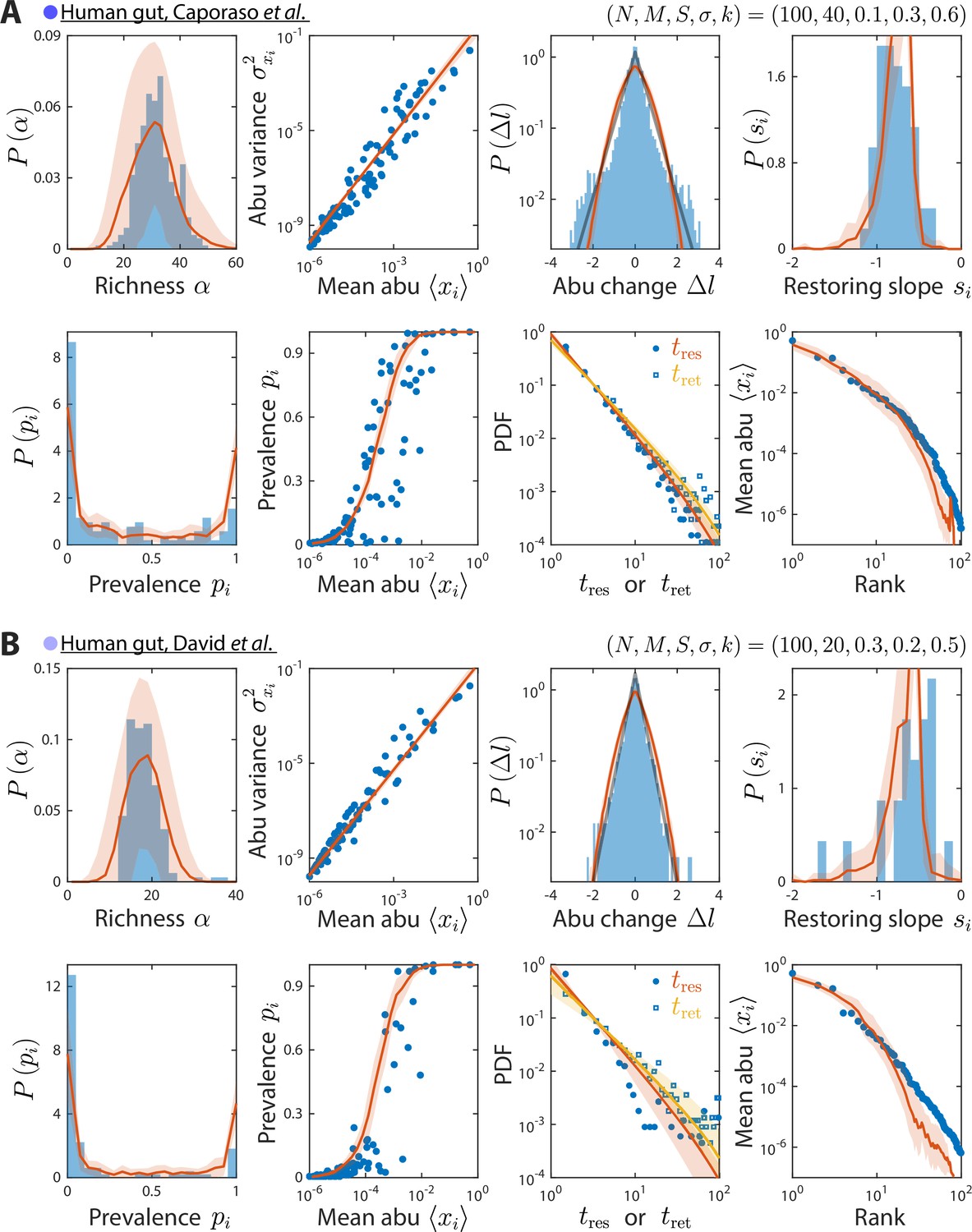
Model reproduces experimentally observed time series statistics in human gut microbiotas.
Shown are the same time series statistics as in Figure 2 for representative data sets (blue) from Caporaso et al., 2011 (A) and David et al., 2014 (B) and best fit model predictions (red).
Figure 5—figure supplement 2
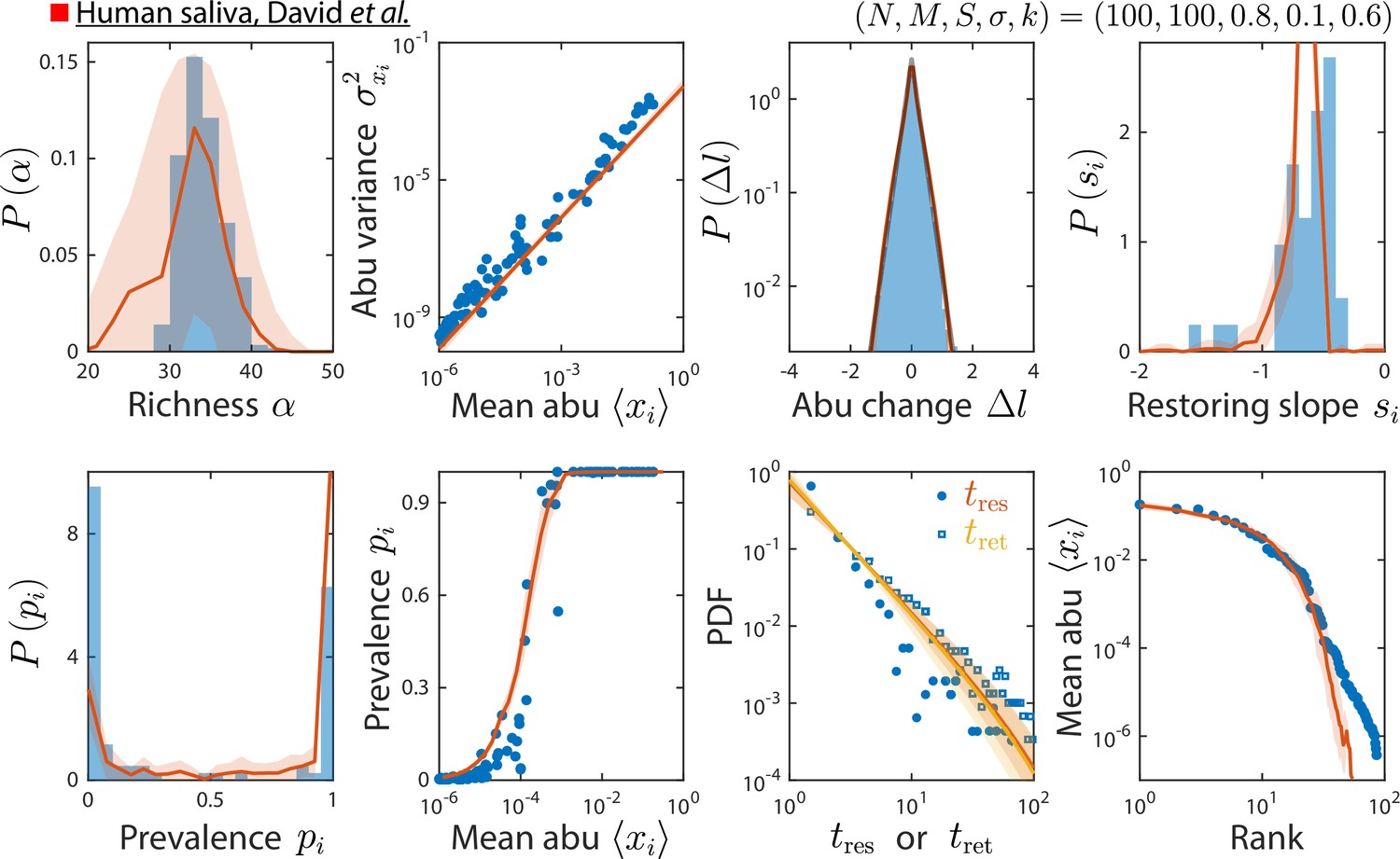
Model reproduces experimentally observed time series statistics in a human saliva microbiota.
Shown are the same time series statistics as in Figure 2 for an experimental data set (blue) from David et al., 2014, and best fit model predictions (red).
Figure 5—figure supplement 3
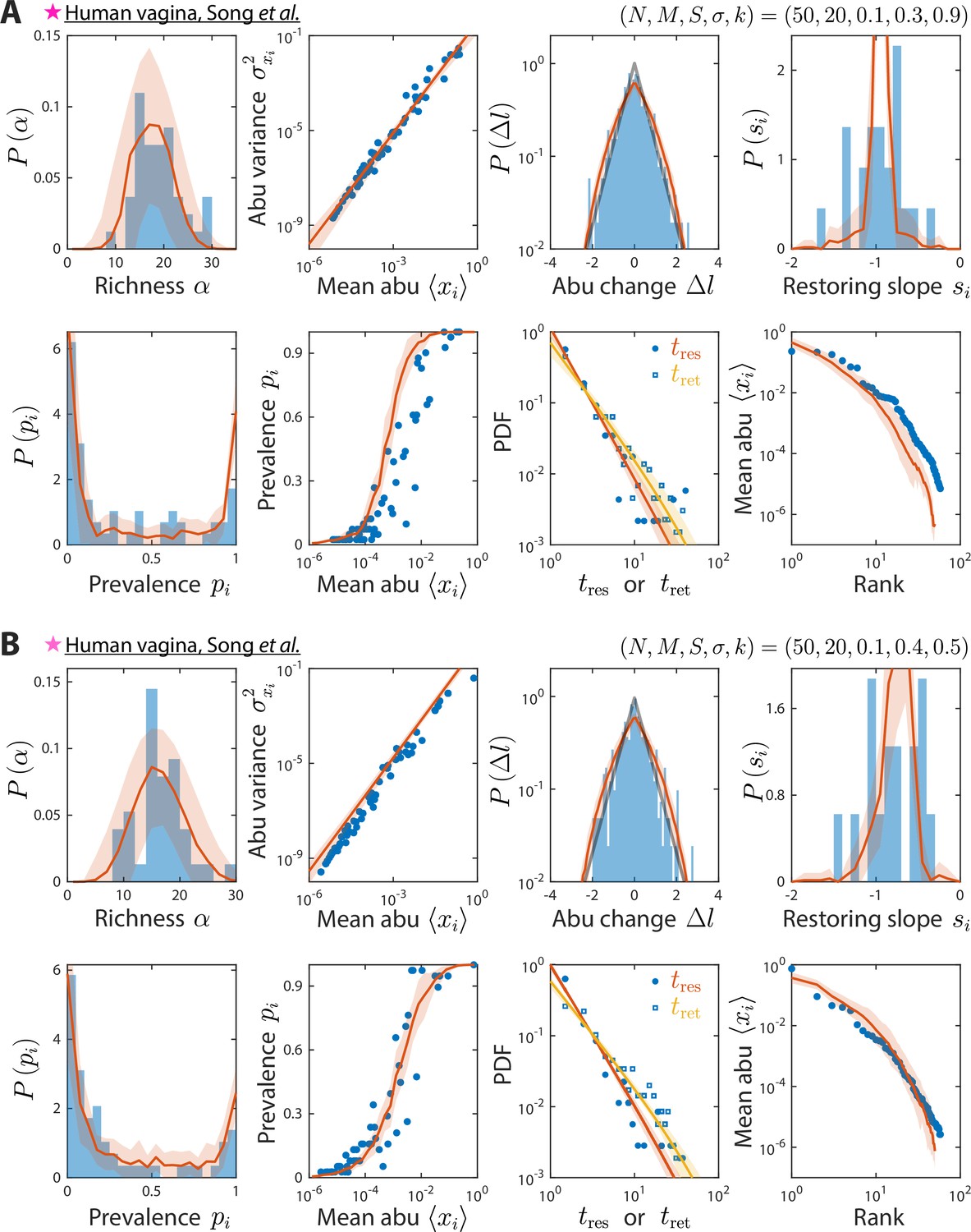
Model reproduces experimentally observed time series statistics in human vagina microbiotas.
Shown are the same time series statistics as in Figure 2 for representative data sets (blue) of vaginal microbiotas with high diversity (A) and dominated by Lactobacillus iners (B) from Song et al., 2020, and best fit model predictions (red).
Figure 5—figure supplement 4

Model reproduces experimentally observed time series statistics in mice gut microbiotas.
Shown are the same time series statistics as in Figure 2 for representative data sets (blue) of mice fed a low fat (A) and high fat diet (B) from Carmody et al., 2015, and best fit model predictions (red).
Figure 5—figure supplement 5

Model reproduces experimentally observed time series statistics in rice microbiotas.
Shown are the same time series statistics as in Figure 2 for representative data sets (blue) of the rhizoplane (A) and endosphere (B) from Edwards et al., 2018, and best fit model predictions (red).
Figure 5—figure supplement 6
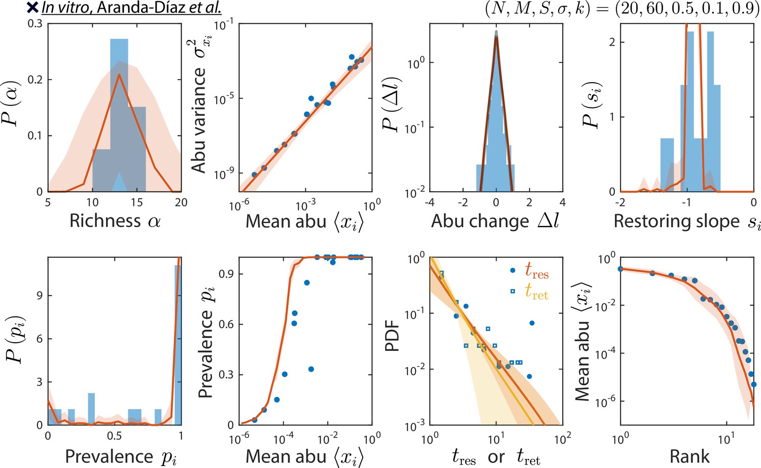
odel reproduces experimentally observed time series statistics in an in vitro-passaged complex community.
Shown are the same time series statistics as in Figure 2 for representative data (blue) from Aranda-Díaz et al., 2022, and best fit model predictions (red).
Author response image 1
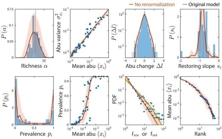
Taxa below the limit of detection do not affect time series statistics.
Shown are data from Caporaso et al. as in Figure 2. The original analysis is shown as dotted black lines. Colored lines denote model predictions without renormalizing the relative abundances after ignoring taxa with relative abundance below the detectability threshold of 10-4; the two lines are virtually indistinguishable in every case.
Additional files
Download links
A two-part list of links to download the article, or parts of the article, in various formats.
Downloads (link to download the article as PDF)
Open citations (links to open the citations from this article in various online reference manager services)
Cite this article (links to download the citations from this article in formats compatible with various reference manager tools)
Competition for fluctuating resources reproduces statistics of species abundance over time across wide-ranging microbiotas
eLife 11:e75168.
https://doi.org/10.7554/eLife.75168


