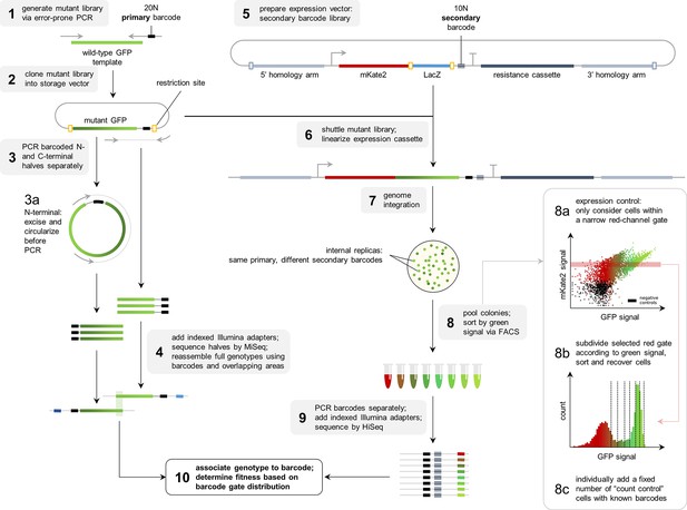
Heterogeneity of the GFP fitness landscape and data-driven protein design
Figures
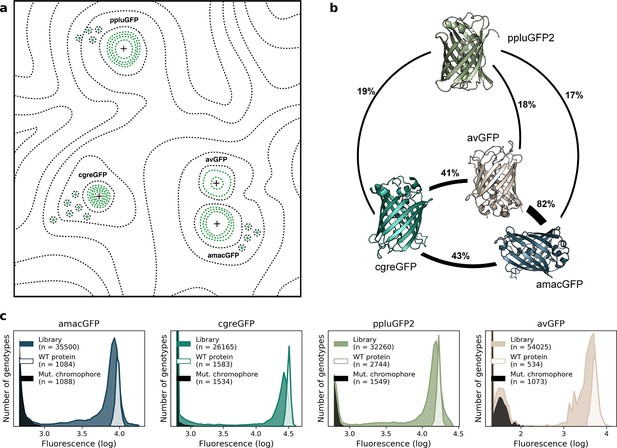
Comparison of four GFP fitness peaks.
(a) A conceptual representation of the GFP fitness landscape following the visualization proposed by Wright, 1932. The black dotted lines represent the unknown regions of the fitness landscape and the green lines the surveyed local fitness peak. Wildtype GFPs (black +) and the predicted functional GFPs (green +) are shown at an approximate scale of sequence divergence from each other. Between the four wildtype fitness peaks there must also be some unknown but large number of other functional and wildtype GFP sequences. For clarity, we do not draw them in the figure. (b) Amino acid sequence identity between different orthologs, displayed in percent. (c) Distribution of fluorescence of mutant libraries (colour), control wildtype protein sequences (white), and protein sequences containing loss-of-function mutations in the chromophore (black).

Distributions of wild-type protein genotypes with and without synonymous mutations.
Fluorescence level distributions of individual barcodes linked to wild-type nucleotide sequences (colour) versus sequences containing only synonymous mutations (dotted line). The minimum number of observations per barcode was 50. The differences between barcoded wildtypes and synonymous variants in all four libraries was not significant (p-value >0.17, two-tailed Mann Whitney U-test).
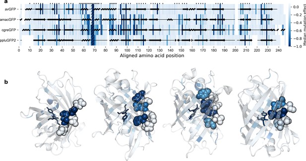
Effects of mutations across the GFP sequences.
(a) Median effects of single mutations according to sequence position. Amino acid residues on one single strand of the beta barrel of GFP monomers. The chromophore sites are hatched (positions 67–69) and sites with buried amino acid side chains are labeled with tick marks. The overlaid protein secondary structure was obtained with Pymol from the respective crystal structures. (b), Median effects of single mutations visualized on protein 3D structures, left-to-right: avGFP (2WUR), amacGFP (7LG4), cgreGFP (2HPW), and ppluGFP2 (2G3O). In each case, a single example beta sheet is represented as spheres in order to better illustrate the difference in mutational effects on residues with internally- versus externally-oriented side chains.

Mutational bias in datasets generated from different mutagenesis strategies.
(a) Observed frequencies of nucleotide mutation types in the four landscapes. Libraries of amacGFP, cgreGFP, and ppluGFP2 were generated with the Mutazyme II kit under the same conditions while the avGFP library was generated by Sarkisyan et al., 2016 employing different dNTP ratios with an in-house error-prone polymerase. ‘Subsampled avGFP’ refers to subsets of 15,000 genotypes of the avGFP library, sampled to mimic the mutational patterns of the Mutazyme-generated libraries. (b) Median brightness of genotypes as a function of the number of nucleotide mutations. Black X marks indicate the values for the complete avGFP dataset, and the colored line shows the values for the subsampled datasets whose mutational patterns are shown in the hatched bars in (a). Error bars indicate standard deviation for 100 simulations. The horizontal red line indicates the threshold used in Sarkisyan et al., 2016, under which genotypes were considered non-functional. (c) Fractions of non-synonymous mutations which result in a significant change in the chemical properties (Creighton and Creighton, 1993) of the amino acid. With the exception of histidine (aromatic and positively charged), we considered amino acids as belonging to one of six categories: positively charged (Arg, Lys, His), negatively charged (Glu, Asp), polar uncharged (Ser, Thr, Gln, Asn), aromatic (Tyr, Trp, Phe, His), aliphatic (Ala, Iso, Leu, Met, Val), and other (Gly, Pro, Cys). A type change was considered to occur when a mutation resulted in the new amino acid belonging to a different category from the original. The difference in percentages between the avGFP ratios and the average amacGFP/cgreGFP/ppluGFP2 ratios were not statistically significant (Fisher’s exact test, P=0.3).
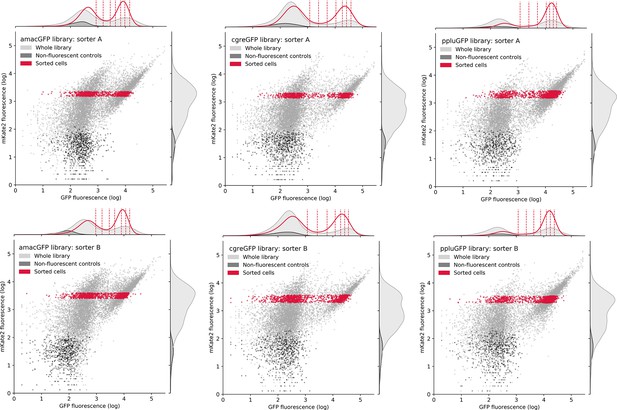
Distribution of cells during FACS sorting.
Entire mutant libraries are shown in grey, non-fluorescent negative controls are shown in black. Sorted cells, falling within the selected gate in the mKate2 channel and corresponding to around 10% of all bacterial cells, are shown in red. Vertical dashed lines in the upper histogram indicate the eight gates in the green channel that cells were recovered from. The histograms indicate the distribution of cells in a single channel.
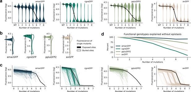
Distributions of fluorescence.
(a) Fluorescence level distributions of genotypes at varying distances from the wildtype and the logistic curves fitted to the median fluorescence for each category (black line). (b), Distribution of fluorescence of genotypes with a single amino acid mutation at exposed (colour) versus buried (white) sites. (c) Starting from genotypes with one mutation away from the wildtype sequence, each line represents the median fluorescence as a function of sequence divergence away from such genotypes. Only points with at least 15 available genotypes are shown. The median fluorescence level at varying distances for the wildtype sequence, black lines, are shown for comparison. (d) The fraction of genotypes without epistasis was calculated as the ratio of the number of observed functional genotypes divided by and the number of genotypes expected to be functional under the assumption of no epistatic interactions between amino acid sites. In the absence of epistasis, the expectation is a constant value of 100% independent of the number of amino acid changes relative to the wildtype.
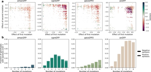
Epistatic interactions of mutations in GFP.
(a) Epistasis in genotypes with two mutations, highlighting negative epistatic interactions between individually neutral or slightly deleterious mutations. The values of impact on fluorescence have an upper and a lower bound. For example, when two mutations that each have an effect of –1.2 (they reduce fluorescence to zero) are present in a single genotype their expected additive effect is still –1.2 because a GFP cannot have a fluorescence less than zero. Thus, negative epistasis is observed for mutations with a weak effect and cannot be observed for strongly deleterious mutations. (b) Fraction of genotypes that display strong epistasis (>1 or 10-fold change) at different distances from the wildtype.
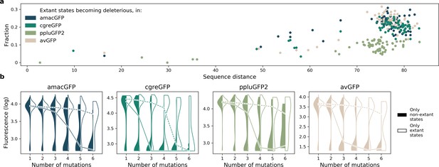
Effect of extant and non-extant mutations.
(a) Fraction of wildtype states in extant green fluorescent proteins which become deleterious in our data, as a function of the sequence divergence (from 0 to 100) between the two proteins. (b) Distribution of fitnesses of mutant genotypes containing only known extant states, or containing no known extant states, at increasing distances from the reference.
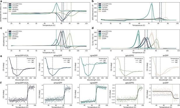
Thermal sensitivity of GFP orthologs.
(a) Thermal unfolding measured by differential scanning fluorimetry (DSF) showing the first derivative of the ratio of 350/330 nm emission. Shaded areas indicate standard deviation of triplicates. (b) Melting curves of green fluorescence emission (510 nm) as a function of temperature measured on a qPCR machine. Shaded areas indicate standard deviations of eight technical replicates. (c) Thermal aggregation measured by DSF showing the first derivative of the light scattering. Shaded areas indicate standard deviation of triplicates. (d) Specific heat capacities measured by differential scanning calorimetry in duplicate. (e) Circular dichroism (CD) spectra measured before (30 °C) and after (98 °C) with the melting curves depicted in (f) where vertical dotted lines indicate the monitored wavelength in (f). f, CD melting curves monitored at 218 nm (and additionally 208 nm in the case of avGFP, where 218 nm did not show a transition), fitted with a logistic curve. In (a), (b), (c), (d), (f), vertical dashed lines indicate the melting temperature, except ppluGFP2 in (b). In (a), (b), (d), (f), temperature was increased at a rate of 1 °C per minute, in (c), at a rate of ~2 °C per minute, the slowest allowed by the LightCycler.
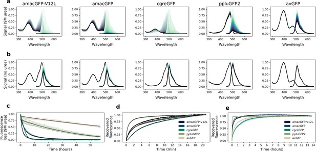
Urea denaturation and refolding of orthologues.
(a) Absorbance (grey) and fluorescence (green) spectra of purified protein in 9 M urea, or (b), 1 x PBS, measured at 42 °C every 30 min for 60 hr; darker lines correspond to later time points. Plotted values are the means of eight technical replicates. (c), Decrease in fluorescence over time during exposure to 9 M urea. avGFP and ppluGFP2 fluorescence loss curves are fitted with one exponential function (f(x) = ), amacGFP and amacGFP:V12L curves are fitted with two exponential functions (black lines), while a good fit using only exponential functions could not be achieved for cgreGFP. Data points from eight technical replicates are shown. (d, e), Fluorescence recovery curves of 9M-urea-denatured proteins upon dilution with 20 volumes of 1 x PBS. Fluorescence (excitation 485 nm, emission 520 nm) was measured every second for twenty minutes in (d), and every 50 s for over 13 hours in (e). Values are normalized to the end points. Recovery curves in (d) were fitted with three exponential functions (black). Shaded areas in (e) represent standard deviations of six technical replicates.
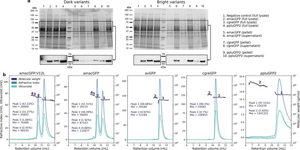
Aggregation and oligomeric states in GFP orthologues.
(a) Coomassie-stained gels (top) of full lysate, pellet, and supernatant of pooled functional (bright) or non-functional (dark) genome-integrated library variants for amacGFP, cgreGFP, and ppluGFP2. Western blot (bottom) of the same samples using an anti-His-tag antibody, showing different aggregation tendency (i.e. pellet localization) for dark versus bright variants. Expected molecular weight of the mKate2-GFP fusion is 53–56 kDa depending on the GFP ortholog. Negative controls are cells of the same strain, but without integrated GFP constructs. Lane identity in both gels is the same, and displayed on the right. (b) SEC-MALS analysis of wild-type proteins, showing protein peaks. Peak analysis is consistent with the following oligomeric states for each gene: amacGFP: primarily mono- and dimeric, with small fractions of tri- and/or tetramers; avGFP: primarily monomeric, with a small dimeric fraction; cgreGFP: primarily dimeric, with a small tetrameric fraction; ppluGFP2: primarily tetrameric, with a small fraction forming large aggregates or oligomers. Mw/Mn ratios for all peaks were between 1 and 1.002, with the exception of the large ppluGFP2 aggregates (Mw/Mn = 1.147).
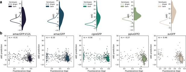
Correlation between fluorescence and ddG predicted by Rosetta.
(a) Distribution of ddG predictions for single mutations observed to either maintain wildtype-level fluorescence (white) or render a genotype non-functional (color). Differences between the two distributions were found to be significant for all genes (Two-tailed Mann Whitney U test, p=0.02 for amacGFP:V12L, and p<0.00002 for all other genes). ddG predictions for mutations to and from proline and glycine were not considered. (b), Correlation between ddG predictions and observed fluorescence of single mutations. The indicated Spearman’s rank correlation coefficient (r) was significant for all genes (p<7 · 10–15).
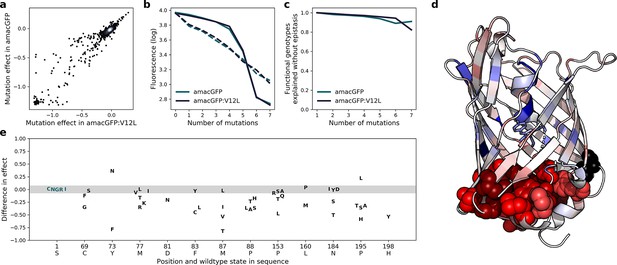
Effects of mutations in amacGFP and amacGFP:V12L.
(a) Correlation between effects of specific mutations in amacGFP backgrounds with and without the V12L (position 14 in our alignment) mutation (Pearson’s r=0.96). (b), Median (solid lines) and mean (dashed lines) fluorescence values of genotypes as a function of the number of mutations relative to amacGFP or amacGFP:V12L sequences. (c), Fraction of observed fluorescent genotypes versus expected to be fluorescent under the assumption of no epistasis as a function of the number of mutations away from amacGFP and amacGFP:V12L. (d), Median difference of the effect of mutations in amacGFP:V12L relative to amacGFP, colored on the crystal structure of amacGFP. Position 12 is colored black. Residues, mutations of which have a stronger effect in amacGFP:V12L are red, those in which the effect of the mutation is stronger in amacGFP are blue. Atoms of residues with a median difference <−0.1 are shown as spheres. (e) Differences in mutation effect between amacGFP:V12L and amacGFP, at the 12 most affected positions. The majority of mutations have a difference in effect between –0.07 and 0.07 (shaded region, for reference see position 1 S).
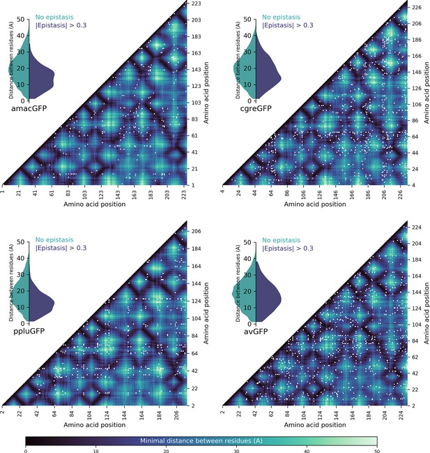
Spatial proximity of amino acid residues and detected pairwise epistasis.
Heatmaps show the minimal distance in Angstroms between two residues, with pairs showing epistatic interactions >0.3 (representing twofold change in fluorescence compared to the additive expectation) shown by white dots. Inset violin plots show the distribution of distances between non-epistatic (green) and epistatic (blue) pairs; in all four cases, the epistatic pairs tended to be physically closer (Two-sided Mann-Whitney U-test, p<10–13).
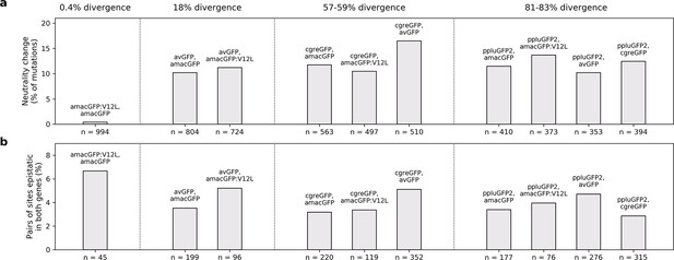
Differences in mutational effects in GFP orthologues.
(a) The proportion of single amino acid mutations which were observed to be neutral (maintaining fluorescence within two standard deviations of the wildtype level) in one GFP sequence and deleterious (reducing fluorescence by over five standard deviations) in another GFP, out of all mutations surveyed in both. The total number of amino acid states considered is indicated beneath the bars. (b), For each pairwise GFP comparisons, first we selected all pairs of amino acid sites for which epistasis was measured. Then, out of these pairs of sites we calculated the number that had epistasis >0.3 in either of the two GFP genes (reported underneath each bar). Finally, we calculated the percent of epistatically interacting sites that were measured to be epistatically interacting in both (y-axis). In (a) and (b), pairs of genes are arranged in order of increasing sequence divergence.
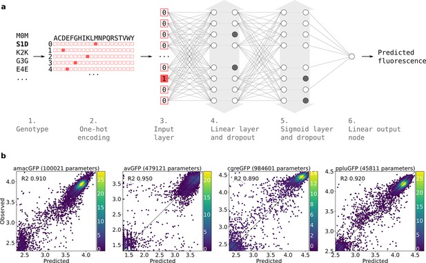
Neural network structure.
(a) 1. Each genotype in the dataset was denoted by the mutations it contained relative to its parental wildtype sequence. 2. Genotypes were one-hot encoded. For each position in the sequence, a binary vector indicated present (red = 1) and absent (white = 0) amino acid states. 3. One-hot encoded sequences were flattened and provided to the neural network as input. 4. The first hidden layer contained linear nodes followed by a dropout layer of the same size. 5. The second hidden layer contained sigmoid nodes followed by a dropout layer of the same size. Grey arrows indicate layer widths that were optimised by a random search. Greyed-out neurons without output connections represent randomly inactivated neurons in dropout layers. During training, randomly inactivated neurons prevented overfitting. At inference time, randomly inactivated neurons allowed the model to provide different estimates of the fluorescence each time a prediction was run on a genotype. 6. Linear node outputting predicted fluorescence values. For each predicted genotype, the median of several fluorescence estimates was used as the final fluorescence level. (b) Correlations between observed and predicted levels of fluorescence with an optimized architecture. Datapoint density is represented in color.
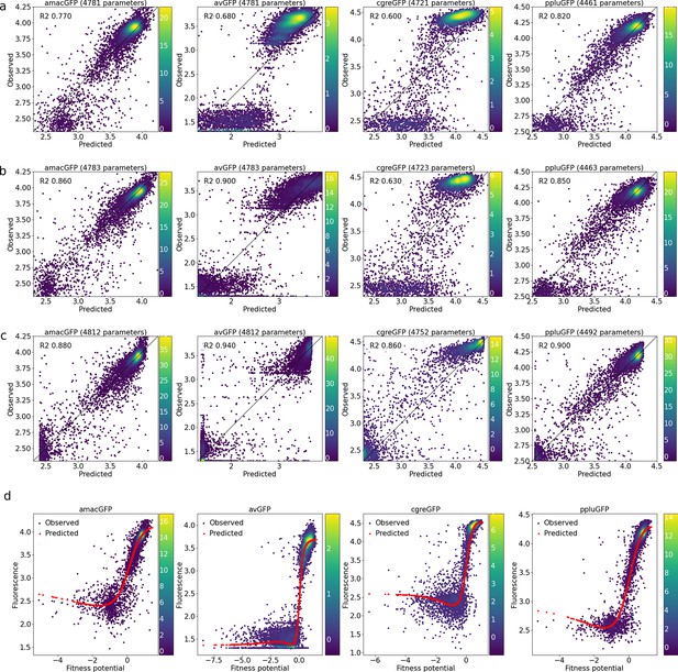
Correlations between observed and predicted levels of fluorescence.
(a) With a linear model, (b), with a linear model and a sigmoid output node, (c), with an output subnetwork, and (d), non-trivial sigmoidal functions transform fitness potentials into predicted fluorescence. Datapoint density is represented in color.
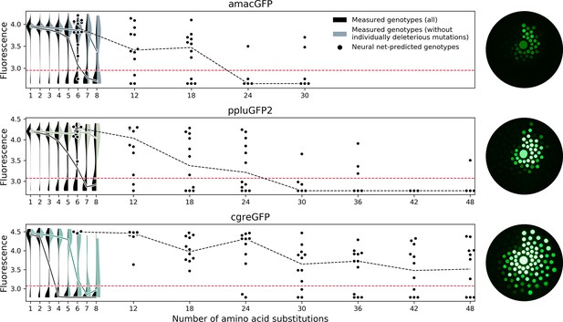
Predicting functional GFP mutants.
Violin plots show the distribution of fluorescence of all genotypes (black) and combinations of only individually neutral mutations (color). Experimental measurements of the level of fluorescence in genotypes predicted by the neural network are shown as black dots (12 genotypes per distance). Black dashed lines show the median fluorescent values for each group. Red dashed lines indicate the cutoff of detectable fluorescence. Photos of agar plates with E. coli spots expressing predicted GFP variants are shown on the right. Spots of bacteria expressing GFP variants are arranged in circles around the wildtype gene at increasing distance with the number of mutations (6, 12, 18, 24, 30, 36, 42, 48 mutations). For each group of genotypes, the brightest ones were inoculated at the top, with fluorescence decreasing clockwise.

Mutations used in machine learning-generated genotypes.
(a) For all genotypes generated by the neural network model (see Figure 5), we show the measured fluorescence as a function of the strongest deleterious effect of any mutation in that genotype that was measured in any genotype in the initial library. In the library of genotypes, individual mutations were observed in multiple genetic contexts, allowing for the measurement of their effect in different backgrounds. Many mutations were neutral in some contexts but deleterious in others. The X axis shows, for each neural network-generated genotype, the strongest deleterious measured effect of any mutation in that genotype. Each colored dot represents one genotype. The threshold for functionality is shown by the dashed red line. (b) In functional neural net-generated genotypes, the proportion of the mutations which were observed to be deleterious (causing over two-fold loss of fluorescence) in at least one genetic context in our data. The total number of mutations used in functional predictions is indicated below the gene name.
Tables
The dataset in numbers.
The avGFP data is from Sarkisyan et al., 2016.
| Gene | amacGFP | cgreGFP | ppluGFP2 | avGFP |
|---|---|---|---|---|
| Number of protein genotypes surveyed | 35,500 | 26,165 | 32,260 | 51,715 |
| Average (median) number of AA substitutions per genotype | 4.37 (3) | 4.23 (3) | 3.7 (2) | 3.93 (4) |
| Average (median) number of barcode replicates per protein genotype | 8.7 (5) | 6.8 (5) | 12 (7) | 1.2 (1) |
| Amino acid identity | avGFP: 82% cgreGFP: 43% ppluGFP2: 17% | avGFP: 41% amacGFP: 43% ppluGFP2: 19% | avGFP: 18% amacGFP: 17% cgreGFP: 19% | amacGFP: 82% cgreGFP: 41% ppluGFP2: 18% |
| False positive rate* | 0.55% (9 of 1635) | 0.75% (14 of 1860) | 0.49% (11 of 2242) | 0.24% (2 of 839) |
| False negative rate* | 0% (0 of 1084) | 0% (0 of 1583) | 0% (0 of 2744) | 0.08% (2 of 2444) |
| Mean wildtype log10 fluorescence level ± standard deviation | 3.97±0.031 (3.96±0.030 for amacGFP:V12L) | 4.50±0.028 | 4.23±0.027 | 3.72±0.082 |
| Fraction of genotypes in which epistasis cannot be ascertained† | 7.4% | 15.9% | 4.5% | 16.5% |
| Fraction of genotypes displaying |epistasis|>0.3 (>1) ‡ | 5.3% (0.2%) | 14.4% (5.6%) | 6.8% (0.9%) | 21.4% (11.6%) |
| Mutational LD50, loss of function § | 5.8 (5.7 for amacGFP:V12L) | 3.2 | 6.2 | 4.1 |
| Mutational LD50, loss of wildtype-level fluorescence level § | 1.7 (1.8 for amacGFP:V12L) | 0.9 | 1.7 | 2.2 |
| Proportion of machine-learning predicted genotypes displaying epistasis <–0.3 (<-1) | 78% (46%) | 57% (21%) | 81% (64%) | NA |
-
*
False positive rates refer to the fraction of genotypes which are expected to be dark or dim due to chromophore mutations but which were assigned a bright fitness; false negative rates refer to genotypes encoding wildtype protein which were assigned dim or dark fitnesses.
-
†
Calculation of epistasis requires knowledge of a genotype’s expected fluorescence, i.e. the sum of contributions of individual mutations. For genotypes with multiple mutations, all individual mutations comprising the genotype must have been measured in isolation.
-
‡
An absolute epistasis value of 0.3 or 1 implies a two-fold or ten-fold difference between the observed and expected fluorescence levels, respectively.
-
§
“Mutational LD50, loss of function” refers to the number of mutations at which 50% of genotypes are rendered non-functional (i.e. assigned to the darkest FACS gate), obtained by fitting a logistic curve to the fraction of non-functional genotypes at each mutational step (see values in Supplementary file 1) and solving for f(x)=0.5; “Mutational LD50, loss of wildtype fluorescence level” refers instead to the number of mutations at which 50% of genotypes maintain a fluorescence level within two standard deviations of the WT level.
Biophysical and biochemical characterisation of wildtype GFPs.
| amacGFP:V12L | amacGFP | cgreGFP | ppluGFP | avGFP | |
|---|---|---|---|---|---|
| Unfolding Tm (DSF) | 80.8 °C | 82.6 °C | 74.1 °C | 91.8 °C | 86.8 °C |
| Aggregation Tm (DSF) | 79.5 °C | 82.0 °C | 73.9 °C | 90.2 °C | 86.6 °C |
| Tm (CD) | 80.4 °C | 82.6 °C | 71.2 °C | 86.4 °C | 83.7 °C |
| Transition slope (CD) | 0.86 | 0.72 | 1.27 | 0.63 | 0.67 |
| Tm (DSC) | 80.2 °C | 82.4 °C | 72.9 °C | 90.3 °C | 86.3 °C |
| Enthalpy of denaturation (DSC) | 744 kJ/mol | 768 kJ/mol | 755 kJ/mol | 515 kJ/mol | 1012 kJ/mol |
| Fluorescence loss Tm (qPCR) | 81.1 °C | 82.6 °C | 72.9 °C | - | 87.5 °C |
| Urea denaturation: initial rate* | –0.87 | –0.35 | –0.18 | –0.02 | –0.009 |
| Kinetic parameters for urea denaturation curves* | a1=0.71 k1=0.96 h–1 a2=0.28 k2=0.25 h–1 | a1=0.52 k1=0.54 h–1 a2=0.43 k2=0.12 h–1 | - | a1=0.92 k1=0.02 h–1 | a1=0.92 k1=0.01 h–1 |
| Refolding: initial rate† | 0.01 | 0.01 | 0.000014 | 0.05 | 0.007 |
| Kinetic parameters for refolding curves† | a1=–0.35 k1=0.025 s–1 a2=–0.36 k2=0.005 s–1 a3=–0.38 k3=0.001 s–1 | a1=–0.057 k1=0.057 s–1 a2=–0.39 k2=0.013 s–1 a3=–0.63 k3=0.002 s–1 | a1=0.16 k1=0.036 s–1 a2=–0.45 k2=0.01 s–1 a3=–0.87 k3=0.001 s–1 | a1=–0.32 k1=0.14 s–1 a2=–0.45 k2=0.02 s–1 a3=–0.21 k3=0.003 s–1 | a1=–0.4 k1=0.016 s–1 a2=–0.36 k2=0.001 s–1 a3=–0.31 k3=0.001 s–1 |
| Expected monomer size | 28.1 kDa | 28.1 kDa | 27.4 kDa | 25.7 kDa | 27.9 kDa |
| Primary oligomeric state (SEC-MALS) | Monomer (67%), dimer (31%) | Monomer (51%), dimer (46%) | Dimer (>99%) | Tetramer (>97%) | Monomer (>99%) |
-
*
Curves monitoring loss of fluorescence in 9 M urea were fitted with two exponential functions in the case of amacGFP and amacGFP:V12L and one exponential function for avGFP and ppluGFP2, while cgreGFP fluorescence loss could not be well modeled using only exponential functions (see Figure 4—figure supplement 1). Initial rates were estimated by calculating the derivative at time t=0.
-
†
Curves monitoring the recovery of fluorescence after urea denaturation over the course of 20 minutes were fitted with three exponential functions (see Figure 4—figure supplement 1). Initial rates were estimated by calculating the derivative at time t=0.
Additional files
-
Transparent reporting form
- https://cdn.elifesciences.org/articles/75842/elife-75842-transrepform1-v3.docx
-
Supplementary file 1
Selected statistics of genotypes at different divergence from five GFP sequences.
- https://cdn.elifesciences.org/articles/75842/elife-75842-supp1-v3.docx
-
Supplementary file 2
Data Collection and Refinement Statistics.
- https://cdn.elifesciences.org/articles/75842/elife-75842-supp2-v3.docx
-
Source data 1
Absolute values for the borders between gates in the green channel during sorting, for all genes and machines, and the corrections applied to match values between the machines.
- https://cdn.elifesciences.org/articles/75842/elife-75842-data1-v3.xlsx
-
Source data 2
Dataframes containing the distribution across gates of all primary-secondary barcode combinations, along with their fitted fitness values (see Materials and methods).
Data are not filtered according to cell count, number of replicates, etc. One dataframe per gene and machine.
- https://cdn.elifesciences.org/articles/75842/elife-75842-data2-v3.zip
-
Source data 3
Dataframes linking nucleotide or protein genotypes to their measured fluorescence level (see Materials and methods).
Mutations in genotypes are labeled in the format AiB, where A is the original wildtype state, B is the mutated state, and i is the position (counting starts from Methionine = 0). In the nucleotide dataset, 'n_replicates' refers to the combined number of distinct barcodes representing a genotype and machines it was measured on. In the amino acid dataset, 'n_replicates' refers to the number of synonymous nucleotide sequences measured for each protein sequence. Nucleotide genotypes and amino acid genotypes are on separate tabs in the file.
- https://cdn.elifesciences.org/articles/75842/elife-75842-data3-v3.xlsx
-
Source data 4
Table containing ddG predictions for single mutations in avGFP, amacGFP, amacGFP:V12L, cgreGFP, and ppluGFP2.
Residue positions are labeled starting from 0 (methionine).
- https://cdn.elifesciences.org/articles/75842/elife-75842-data4-v3.csv
-
Source data 5
Dataframes containing the minimum physical distance between pairs of residues inside the 3D GFP structures, in Angstroms.
Row and column indices represent the residue position within the protein, starting from 0 for the initial methionine. Matrices for different proteins are included in different tabs in the file.
- https://cdn.elifesciences.org/articles/75842/elife-75842-data5-v3.xlsx
-
Source data 6
Table containing absorbance values (from 300 to 700nm) and fluorescence emission values (from 450nm to 700nm, upon 420nm excitation) for all genes, in 9M urea and PBS, measured on a plate reader at multiple consecutive time points.
Blank control values are already subtracted. Absorbance and fluorescence data are listed on separate tabs
- https://cdn.elifesciences.org/articles/75842/elife-75842-data6-v3.xlsx
-
Source data 7
Raw data from differential scanning fluorimetry and calorimetry, circular dichroism, and qPCR melting curves.
- https://cdn.elifesciences.org/articles/75842/elife-75842-data7-v3.xlsx
-
Source data 8
Coding sequences for neural network-generated genotypes, and their predicted and observed levels of fluorescence.
- https://cdn.elifesciences.org/articles/75842/elife-75842-data8-v3.csv
-
Source data 9
Table of over 70 documented natural fluorescent proteins used during analyses, including name, species, sequence, original reference and, where possible, accession numbers and measured excitation/emission peaks.
- https://cdn.elifesciences.org/articles/75842/elife-75842-data9-v3.csv
-
Source data 10
Estimated rates of evolution of amino acid states used in prediction of novel GFP sequences on each branch of the phylogeny of extant GFPs.
- https://cdn.elifesciences.org/articles/75842/elife-75842-data10-v3.xlsx


