Evolution-based mathematical models significantly prolong response to abiraterone in metastatic castrate-resistant prostate cancer and identify strategies to further improve outcomes
Figures
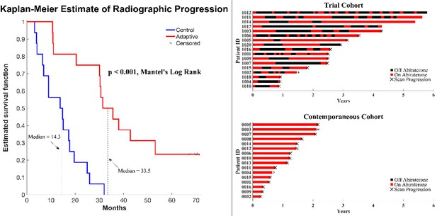
Clinical status of patients in the clinical trial at cutoff date of 01/01/2022.
(Left) Kaplan–Meier curve for time to radiographic progression in the adaptive therapy (n = 17) compared to continuous therapy (n = 16) cohort. Four patients in the adaptive arm remain in the trial with no evidence of progression (time on trial ranging from 52 to 69 months). (Right) Swimmer plot showing times on and off therapy, and clinical outcomes for each patient from both cohorts.

Estimates of key parameters (a, b) and relationship between time to radiographic progression (TTP) and initial population fraction of cancer cells resistant to abiraterone (c).
Parameters αRS (competition coefficient of sensitive on resistant cells) and (growth rate scaling factor) were estimated by a constrained nonlinear multivariable optimization minimizing the least-squares difference between the output of the model and the actual patient data over the entire cohort. The global minimum occurred at αRS = 6 and . (c) TTP declines with the estimated pretreatment fraction of resistant cells for both adaptive therapy and continuous therapy cohorts. Adaptive therapy is superior to continuous therapy. No adaptive therapy patient lies below the regression line for continuous therapy, and no continuous therapy patient lies above the regression line for adaptive therapy.

Based on estimated parameter values, retrospective analyses show that adaptive therapy could have provided disease control for patients on continuous therapy.
For patients C007 (a) and C004 (b), the pretreatment fraction of resistant cancer cells was estimated as 0.3 and 0.25, respectively, and time to radiographic progression was 526 and 128 days, respectively.
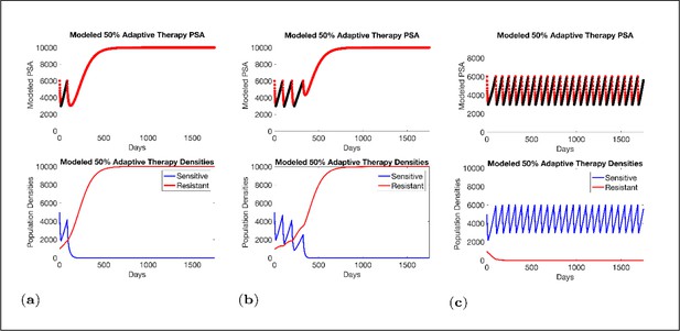
Sensitivity of resistant cell population to the value of the competition coefficient.
In the top panels, we show the ideal cycling of the PSA treatment in which treatment is stopped immediately upon reaching 50% of the pretreatment value and resumed immediately upon reaching that value. In the lower panel, we show computer simulations of changes in the treatment-sensitive (blue) and treatment-resistant populations (red). Treatment dynamics are sensitive to the value of the competition coefficient (αRS), which is dependent on the fitness differences of the sensitive and resistant populations in the absence of treatment. In panel (a) we assume αRS = 0.8 and increase in xS does not decrease the population xR and adaptive therapy fails. In panel (b), αRS = 2, the increase in xS during treatment holidays slows the growth of xR and delays treatment failure. In panel (c) the estimated αRSRS 6 results in a negative growth rate in xR during proliferation of xS. Over 3–4 cycles, the xR population approaches 0. This allows the cycling treatment to maintain tumor control indefinitely. Note that, however, this represents an ideal setting and does not account for other dynamics (see below) that may result in loss of control.
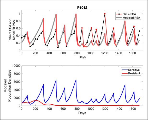
In the upper panel, the dotted line indicates actual PSA measurements.
The red line represents the model fit for the data. In the lower panel, computer simulations estimating the sizes of the treatment-sensitive (blue) and resistant (red) populations over time are demonstrated. Simulations suggest that optimal timing resulted in the elimination of the resistant population in adaptive therapy patients with prolonged survival. Patient 1012 in the adaptive therapy cohort with enduring control (>1800 days). Model simulations suggest that the sequence of 2–4 treatment cycles caused the resistant population to reduce to near extinction permitting a stable cycling regime in which only abiraterone-sensitive cells are present.
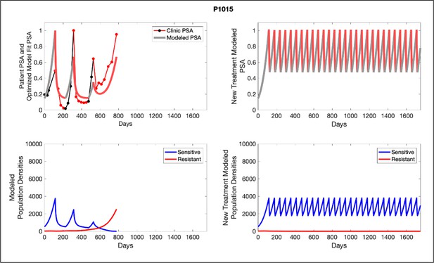
Left panels show actual patient PSA data (dotted line) and computer simulation curve fits (red line in upper panel) and estimated sizes (lower panel) of treatment-sensitive (blue) and resistant (red) populations during treatment.
Right panel represents a computer simulation in which treatment is withdrawn immediately upon reaching the 50% threshold and restarted immediately upon returning to the pretreatment value. Left panel: simulations suggest that unintended, yet excessive, reduction of the sensitive population led to the proliferation and dominance of the resistant population. Right panel: optimizing the timing of withdrawing therapy immediately upon reaching the 50% pretreatment PSA threshold, thereby preventing overtreatment, allows maximal suppression of the resistant population and consistent long-term control in adaptive therapy patients. Of note, allowing the PSA to increase above pretreatment value had no negative consequences because it generally caused a further decline in the resistant population (data not shown).
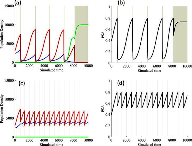
Results from adaptive therapy protocols in which a PSA drop of 80% is required before drug holiday (a) and (b), and in which only a 20% drop is required before drug holiday (c) and (d).
The red is TP cells that are directly affected by administration of abiraterone, blue is the T+ cells, and green is the therapy-resistant T- cells. The regions where the background is highlighted are the times at which abiraterone is being administered.
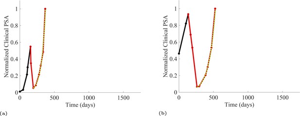
PSA time-series data for patients C005 (a) and C013 (b).
Here, the PSA dynamics are highlighted in red, showing that abiraterone is being administered. The green dotted line shows the fit used to estimate the growth rate of the resistant cell population after progression through abiraterone. As abiraterone is still being administered and cell populations are still growing, we assume that sensitive cells have been eliminated and only abiraterone-resistant cells remain.
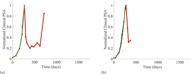
PSA time-series data for patients C014 (a) and C011 (b).
Here, the PSA dynamics are highlighted in red, showing that abiraterone is being administered. The green dotted line shows the fit used to estimate the growth rate of the sensitive cell population before any treatment with abiraterone. As abiraterone has not yet been introduced, this growth is assumed to be completely from the abiraterone-sensitive cells.
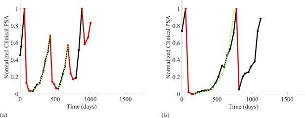
PSA time-series data for patients P1016 (a) and P1017 (b).
PSA dynamics highlighted in red and black show periods of abiraterone therapy on and off, respectively. Green dotted lines show exponential fits to periods when abiraterone was off. These provide estimates for the growth rates of the sensitive cell population during the off treatment period of an adaptive therapy cycle. We obtained two estimated values for P1016 and one for P1017. When off abiraterone, we assume that the growth in tumor burdens comes predominantly from the abiraterone-sensitive cells.
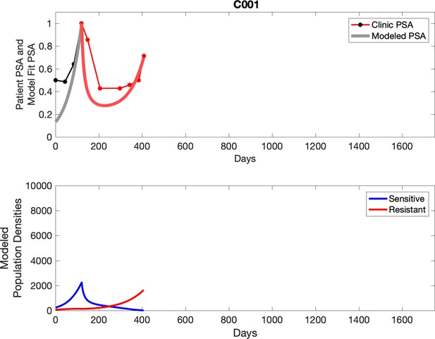
Observed PSA dynamics and model fit for the designated subject are shown in the top panel, and model simulations estimating changes in sensitive and resistant cell populations are in the lower panel.
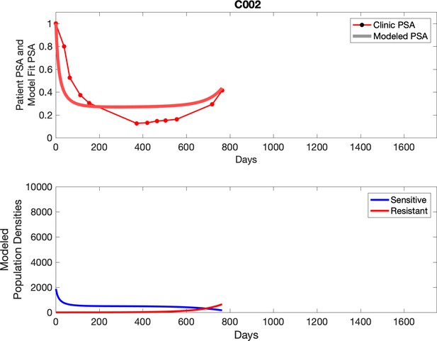
Observed PSA dynamics and model fit for the designated subject are shown in the top panel, and model simulations estimating changes in sensitive and resistant cell populations are in the lower panel.
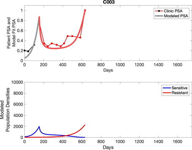
Observed PSA dynamics and model fit for the designated subject are shown in the top panel, and model simulations estimating changes in sensitive and resistant cell population are in the lower panel.
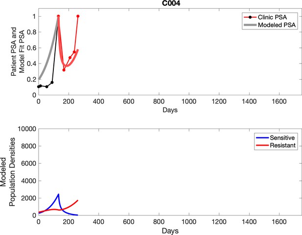
Observed PSA dynamics and model fit for the designated subject are shown in the top panel, and model simulations estimating changes in sensitive and resistant cell population are in the lower panel.
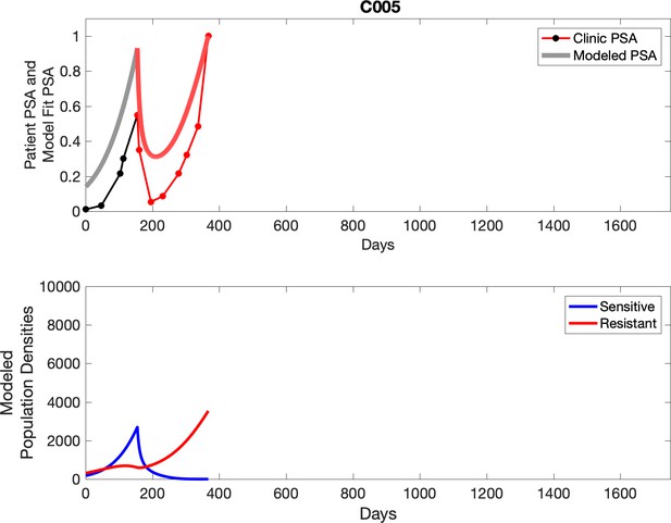
Observed PSA dynamics and model fit for the designated subject are shown in the top panel, and model simulations estimating changes in sensitive and resistant cell population are in the lower panel.
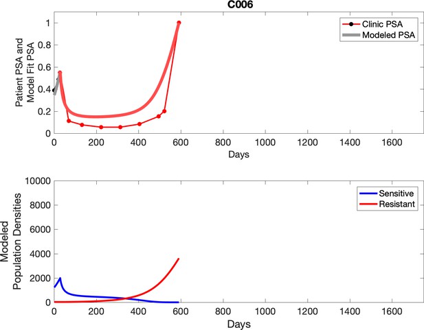
Observed PSA dynamics and model fit for the designated subject are shown in the top panel, and model simulations estimating changes in sensitive and resistant cell population are in the lower panel.
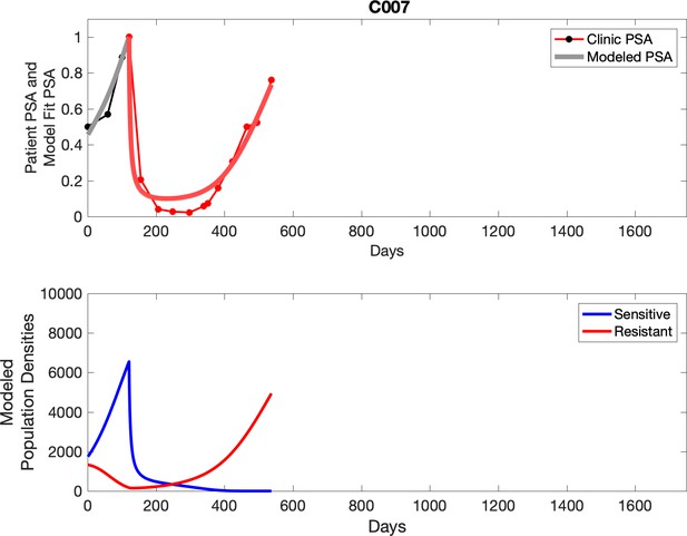
Observed PSA dynamics and model fit for the designated subject are shown in the top panel, and model simulations estimating changes in sensitive and resistant cell population are in the lower panel.
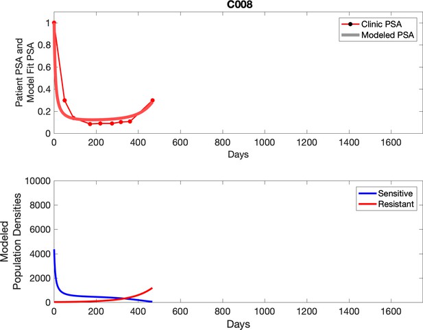
Observed PSA dynamics and model fit for the designated subject are shown in the top panel, and model simulations estimating changes in sensitive and resistant cell population are in the lower panel.
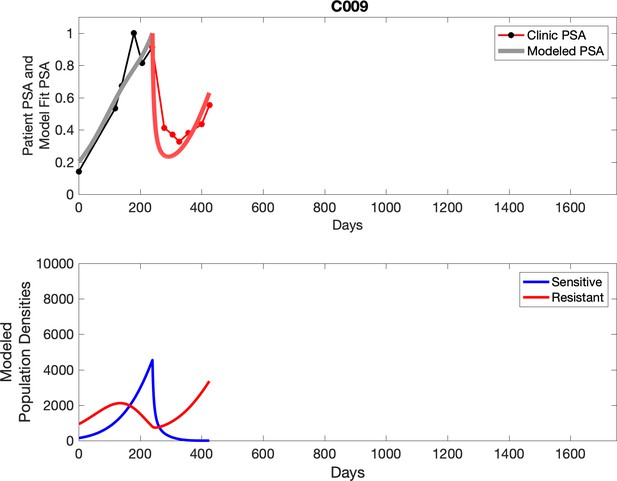
Observed PSA dynamics and model fit for the designated subject are shown in the top panel, and model simulations estimating changes in sensitive and resistant cell population are in the lower panel.
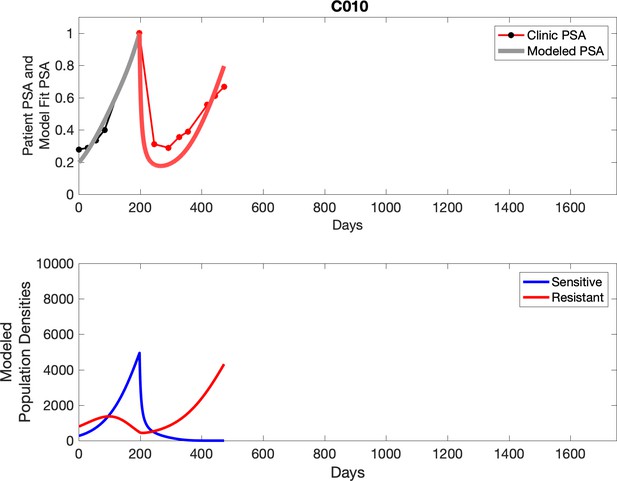
Observed PSA dynamics and model fit for the designated subject are shown in the top panel, and model simulations estimating changes in sensitive and resistant cell populations are in the lower panel.
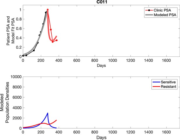
Observed PSA dynamics and model fit for the designated subject are shown in the top panel, and model simulations estimating changes in sensitive and resistant cell populations are in the lower panel.
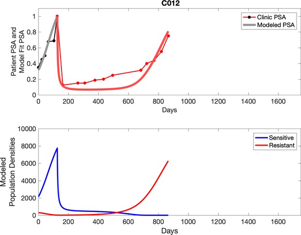
Observed PSA dynamics and model fit for the designated subject are shown in the top panel, and model simulations estimating changes in sensitive and resistant cell populations are in the lower panel.
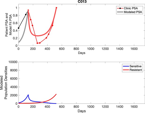
Observed PSA dynamics and model fit for the designated subject are shown in the top panel, and model simulations estimating changes in sensitive and resistant cell populations are in the lower panel.
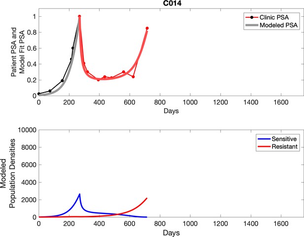
Observed PSA dynamics and model fit for the designated subject are shown in the top panel, and model simulations estimating changes in sensitive and resistant cell populations are in the lower panel.
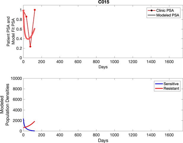
Observed PSA dynamics and model fit for the designated subject are shown in the top panel, and model simulations estimating changes in sensitive and resistant cell population are in the lower panel.
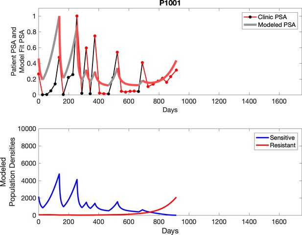
Observed PSA dynamics and model fit for the designated subject are shown in the top panel, and model simulations estimating changes in sensitive and resistant cell populations are in the lower panel.
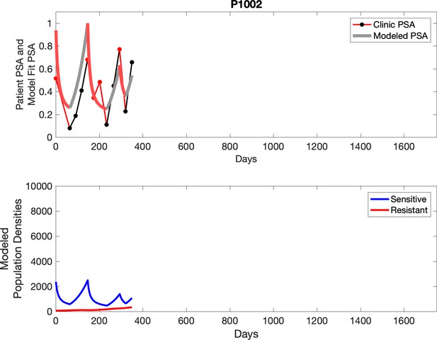
Observed PSA dynamics and model fit for the designated subject are shown in the top panel, and model simulations estimating changes in sensitive and resistant cell populations are in the lower panel.
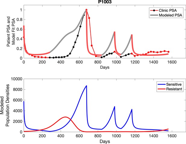
Observed PSA dynamics and model fit for the designated subject are shown in the top panel, and model simulations estimating changes in sensitive and resistant cell populations are in the lower panel.
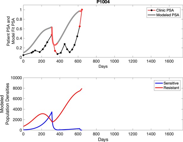
Observed PSA dynamics and model fit for the designated subject are shown in the top panel, and model simulations estimating changes in sensitive and resistant cell populations are in the lower panel.
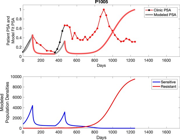
Observed PSA dynamics and model fit for the designated subject are shown in the top panel, and model simulations estimating changes in sensitive and resistant cell populations are in the lower panel.
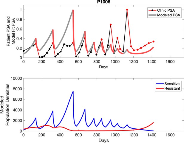
Observed PSA dynamics and model fit for the designated subject are shown in the top panel, and model simulations estimating changes in sensitive and resistant cell populations are in the lower panel.
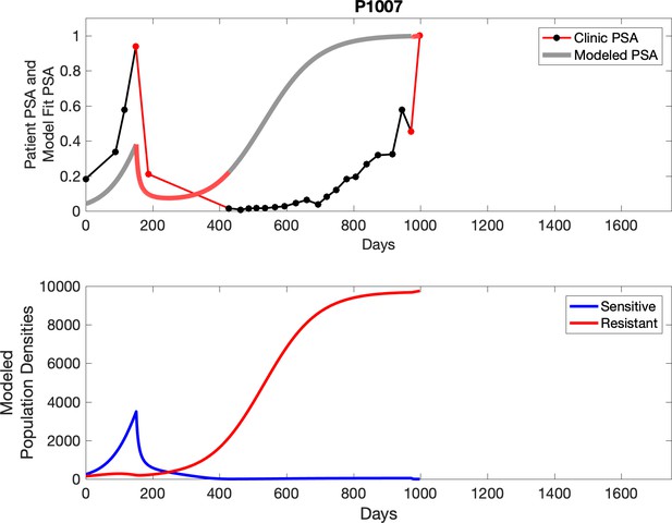
Observed PSA dynamics and model fit for the designated subject are shown in the top panel, and model simulations estimating changes in sensitive and resistant cell populations are in the lower panel.
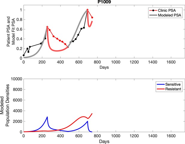
Observed PSA dynamics and model fit for the designated subject are shown in the top panel, and model simulations estimating changes in sensitive and resistant cell populations are in the lower panel.
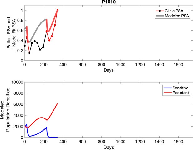
Observed PSA dynamics and model fit for the designated subject are shown in the top panel, and model simulations estimating changes in sensitive and resistant cell populations are in the lower panel.
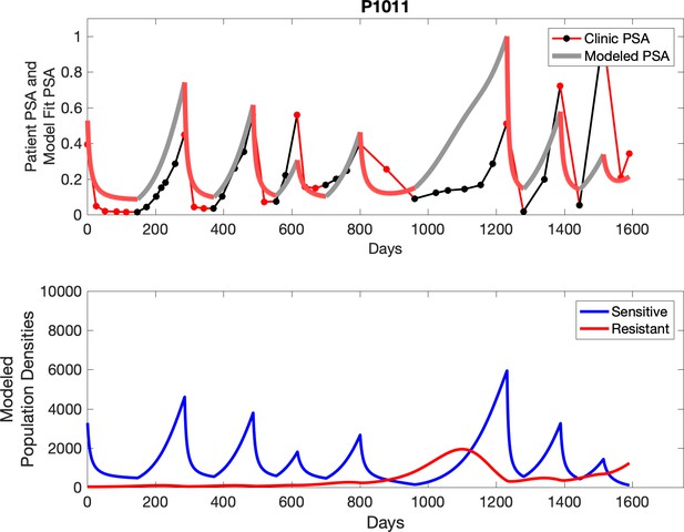
Observed PSA dynamics and model fit for the designated subject are shown in the top panel, and model simulations estimating changes in sensitive and resistant cell populations are in the lower panel.
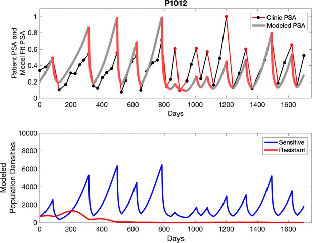
Observed PSA dynamics and model fit for the designated subject are shown in the top panel, and model simulations estimating changes in sensitive and resistant cell populations are in the lower panel.
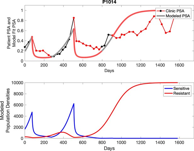
Observed PSA dynamics and model fit for the designated subject are shown in the top panel, and model simulations estimating changes in sensitive and resistant cell populations are in the lower panel.
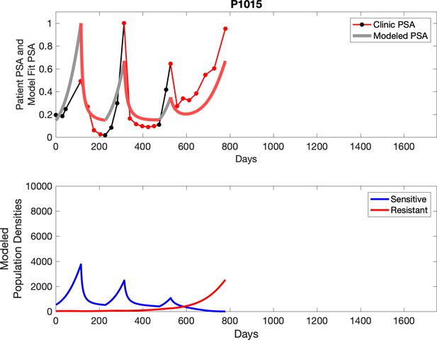
Observed PSA dynamics and model fit for the designated subject are shown in the top panel, and model simulations estimating changes in sensitive and resistant cell populations are in the lower panel.
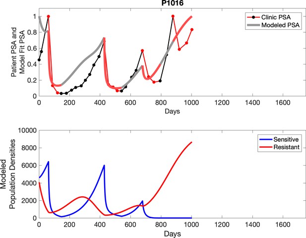
Observed PSA dynamics and model fit for the designated subject are shown in the top panel, and model simulations estimating changes in sensitive and resistant cell populations are in the lower panel.
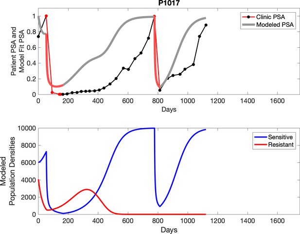
Observed PSA dynamics and model fit for the designated subject are shown in the top panel, and model simulations estimating changes in sensitive and resistant cell populations are in the lower panel.
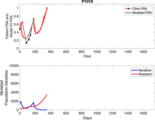
Observed PSA dynamics and model fit for the designated subject are shown in the top panel, and model simulations estimating changes in sensitive and resistant cell populations are in the lower panel.
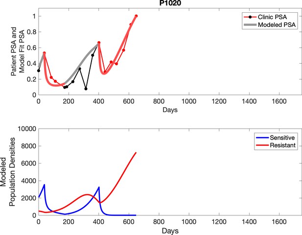
Observed PSA dynamics and model fit for the designated subject are shown in the top panel, and model simulations estimating changes in sensitive and resistant cell population are in the lower panel.
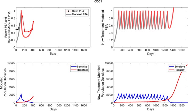
The left column shows actual outcome (upper panel) and computer simulations (lower panel) of the estimated population dynamics of the sensitive and resistant poulations for the indicated subject; the right column shows computer simulations based on an assumption that treatment was stopped immediately when the PSA fell below 0.5 of the pre-treatment and resumed immediately when PSA increased to the pretreatment value.
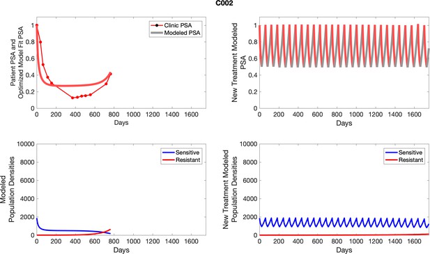
The left column shows actual outcome (upper panel) and computer simulations (lower panel) of the estimated population dynamics of the sensitive and resistant poulations for the indicated subject; the right column shows computer simulations based on an assumption that treatment was stopped immediately when the PSA fell below 0.5 of the pre-treatment and resumed immediately when PSA increased to the pretreatment value.
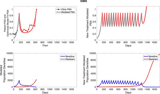
The left column shows actual outcome (upper panel) and computer simulations (lower panel) of the estimated population dynamics of the sensitive and resistant poulations for the indicated subject; the right column shows computer simulations based on an assumption that treatment was stopped immediately when the PSA fell below 0.5 of the pre-treatment and resumed immediately when PSA increased to the pretreatment value.
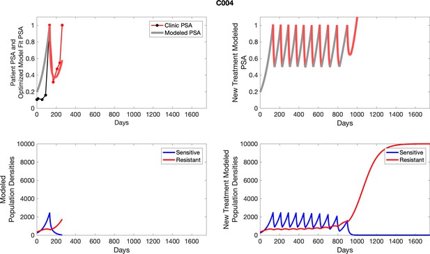
The left column shows actual outcome (upper panel) and computer simulations (lower panel) of the estimated population dynamics of the sensitive and resistant poulations for the indicated subject; the right column shows computer simulations based on an assumption that treatment was stopped immediately when the PSA fell below 0.5 of the pre-treatment and resumed immediately when PSA increased to the pretreatment value.
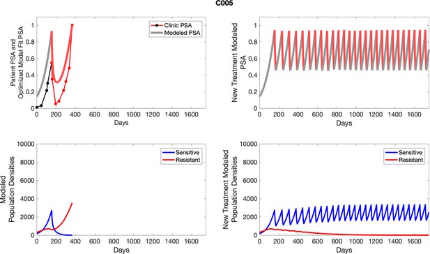
The left column shows actual outcome (upper panel) and computer simulations (lower panel) of the estimated population dynamics of the sensitive and resistant poulations for the indicated subject; the right column shows computer simulations based on an assumption that treatment was stopped immediately when the PSA fell below 0.5 of the pre-treatment and resumed immediately when PSA increased to the pretreatment value.
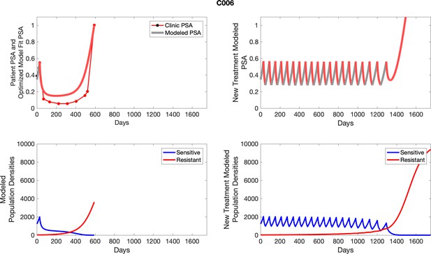
The left column shows actual outcome (upper panel) and computer simulations (lower panel) of the estimated population dynamics of the sensitive and resistant poulations for the indicated subject; the right column shows computer simulations based on an assumption that treatment was stopped immediately when the PSA fell below 0.5 of the pre-treatment and resumed immediately when PSA increased to the pretreatment value.
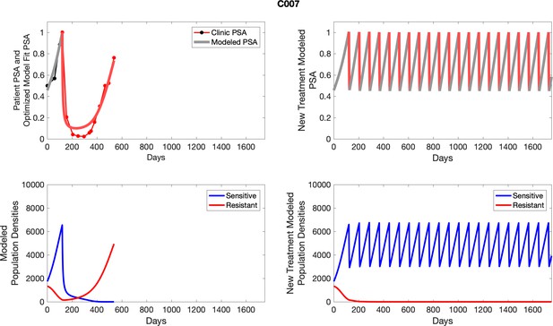
The left column shows actual outcome (upper panel) and computer simulations (lower panel) of the estimated population dynamics of the sensitive and resistant poulations for the indicated subject; the right column shows computer simulations based on an assumption that treatment was stopped immediately when the PSA fell below 0.5 of the pre-treatment and resumed immediately when PSA increased to the pretreatment value.
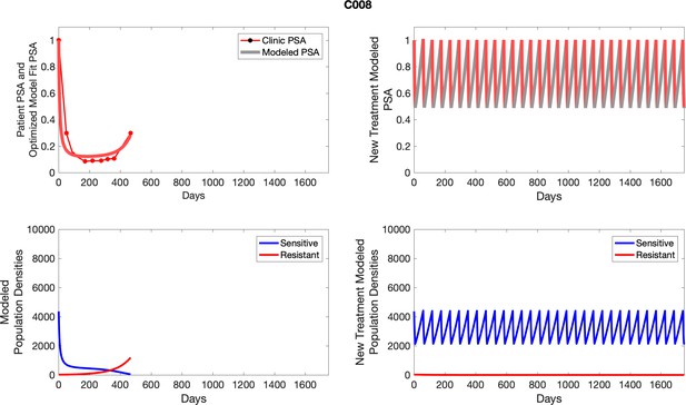
The left column shows actual outcome (upper panel) and computer simulations (lower panel) of the estimated population dynamics of the sensitive and resistant poulations for the indicated subject; the right column shows computer simulations based on an assumption that treatment was stopped immediately when the PSA fell below 0.5 of the pre-treatment and resumed immediately when PSA increased to the pretreatment value.
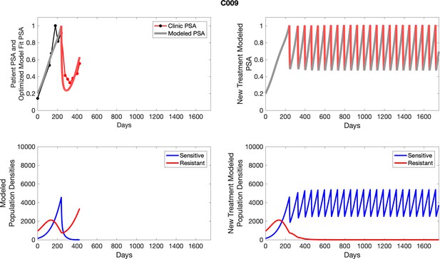
The left column shows actual outcome (upper panel) and computer simulations (lower panel) of the estimated population dynamics of the sensitive and resistant poulations for the indicated subject; the right column shows computer simulations based on an assumption that treatment was stopped immediately when the PSA fell below 0.5 of the pre-treatment and resumed immediately when PSA increased to the pretreatment value.
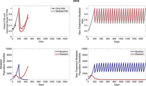
The left column shows actual outcome (upper panel) and computer simulations (lower panel) of the estimated population dynamics of the sensitive and resistant poulations for the indicated subject; the right column shows computer simulations based on an assumption that treatment was stopped immediately when the PSA fell below 0.5 of the pre-treatment and resumed immediately when PSA increased to the pretreatment value.
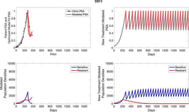
The left column shows actual outcome (upper panel) and computer simulations (lower panel) of the estimated population dynamics of the sensitive and resistant poulations for the indicated subject; the right column shows computer simulations based on an assumption that treatment was stopped immediately when the PSA fell below 0.5 of the pre-treatment and resumed immediately when PSA increased to the pretreatment value.
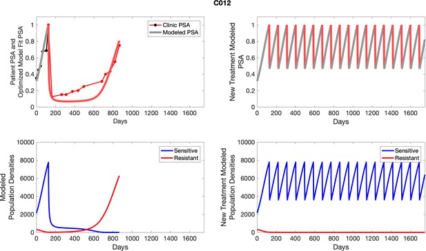
The left column shows actual outcome (upper panel) and computer simulations (lower panel) of the estimated population dynamics of the sensitive and resistant poulations for the indicated subject; the right column shows computer simulations based on an assumption that treatment was stopped immediately when the PSA fell below 0.5 of the pre-treatment and resumed immediately when PSA increased to the pretreatment value.
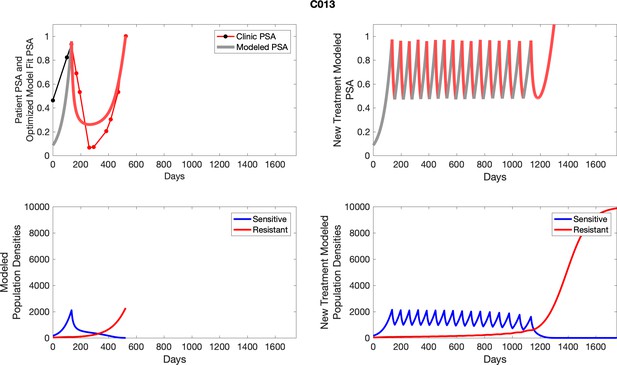
The left column shows actual outcome (upper panel) and computer simulations (lower panel) of the estimated population dynamics of the sensitive and resistant poulations for the indicated subject; the right column shows computer simulations based on an assumption that treatment was stopped immediately when the PSA fell below 0.5 of the pre-treatment and resumed immediately when PSA increased to the pretreatment value.
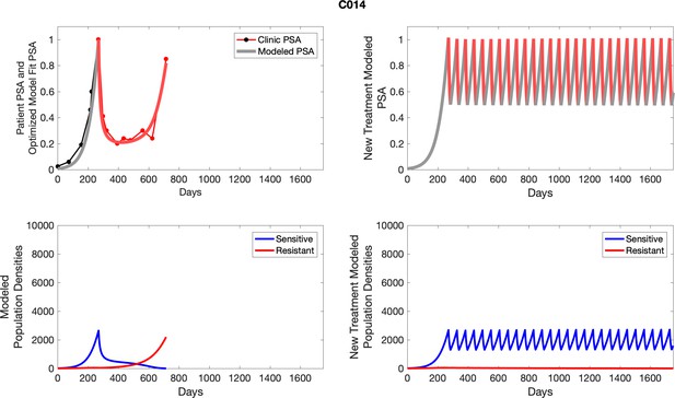
The left column shows actual outcome (upper panel) and computer simulations (lower panel) of the estimated population dynamics of the sensitive and resistant poulations for the indicated subject; the right column shows computer simulations based on an assumption that treatment was stopped immediately when the PSA fell below 0.5 of the pre-treatment and resumed immediately when PSA increased to the pretreatment value.
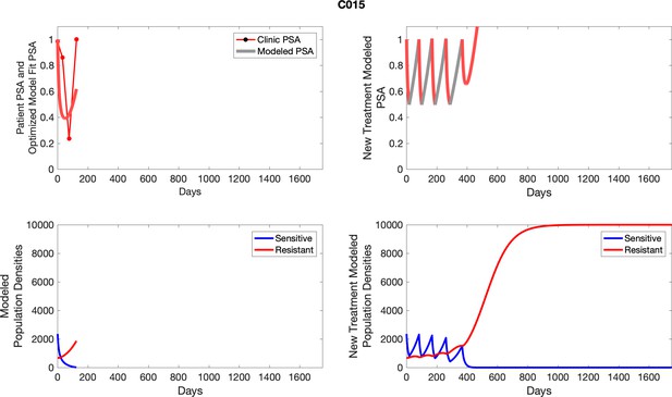
The left column shows actual outcome (upper panel) and computer simulations (lower panel) of the estimated population dynamics of the sensitive and resistant poulations for the indicated subject; the right column shows computer simulations based on an assumption that treatment was stopped immediately when the PSA fell below 0.5 of the pre-treatment and resumed immediately when PSA increased to the pretreatment value.
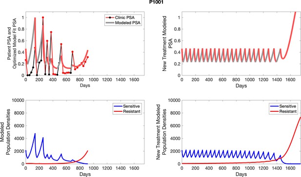
The left column shows actual outcome (upper panel) and computer simulations (lower panel) of the estimated population dynamics of the sensitive and resistant poulations for the indicated subject; the right column shows computer simulations based on an assumption that treatment was stopped immediately when the PSA fell below 0.5 of the pre-treatment and resumed immediately when PSA increased to the pretreatment value.
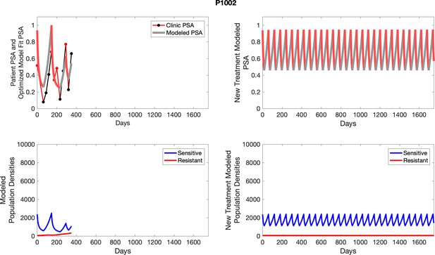
The left column shows actual outcome (upper panel) and computer simulations (lower panel) of the estimated population dynamics of the sensitive and resistant poulations for the indicated subject; the right column shows computer simulations based on an assumption that treatment was stopped immediately when the PSA fell below 0.5 of the pre-treatment and resumed immediately when PSA increased to the pretreatment value.
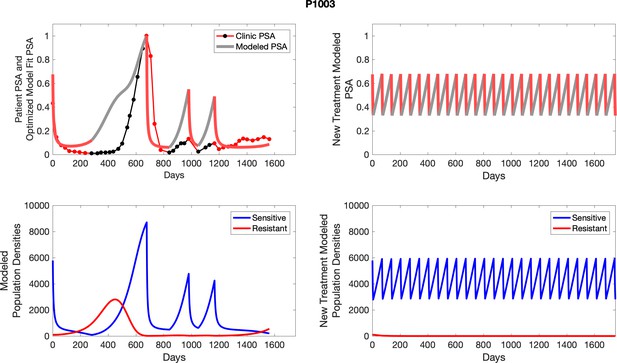
The left column shows actual outcome (upper panel) and computer simulations (lower panel) of the estimated population dynamics of the sensitive and resistant poulations for the indicated subject; the right column shows computer simulations based on an assumption that treatment was stopped immediately when the PSA fell below 0.5 of the pre-treatment and resumed immediately when PSA increased to the pretreatment value.
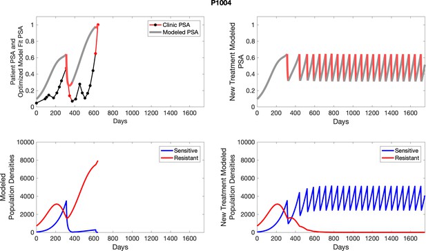
The left column shows actual outcome (upper panel) and computer simulations (lower panel) of the estimated population dynamics of the sensitive and resistant poulations for the indicated subject; the right column shows computer simulations based on an assumption that treatment was stopped immediately when the PSA fell below 0.5 of the pre-treatment and resumed immediately when PSA increased to the pretreatment value.
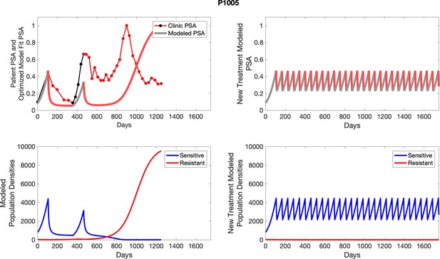
The left column shows actual outcome (upper panel) and computer simulations (lower panel) of the estimated population dynamics of the sensitive and resistant poulations for the indicated subject; the right column shows computer simulations based on an assumption that treatment was stopped immediately when the PSA fell below 0.5 of the pre-treatment and resumed immediately when PSA increased to the pretreatment value.
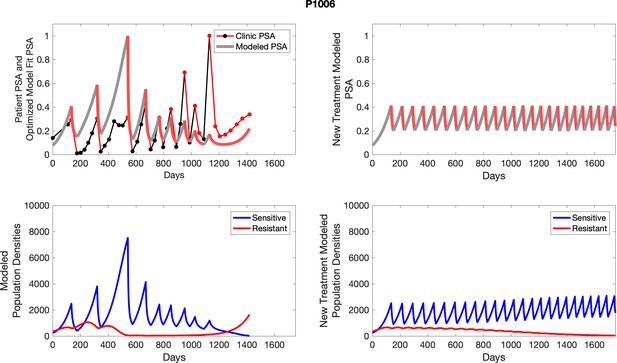
The left column shows actual outcome (upper panel) and computer simulations (lower panel) of the estimated population dynamics of the sensitive and resistant poulations for the indicated subject; the right column shows computer simulations based on an assumption that treatment was stopped immediately when the PSA fell below 0.5 of the pre-treatment and resumed immediately when PSA increased to the pretreatment value.
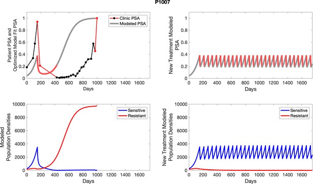
The left column shows actual outcome (upper panel) and computer simulations (lower panel) of the estimated population dynamics of the sensitive and resistant poulations for the indicated subject; the right column shows computer simulations based on an assumption that treatment was stopped immediately when the PSA fell below 0.5 of the pre-treatment and resumed immediately when PSA increased to the pretreatment value.
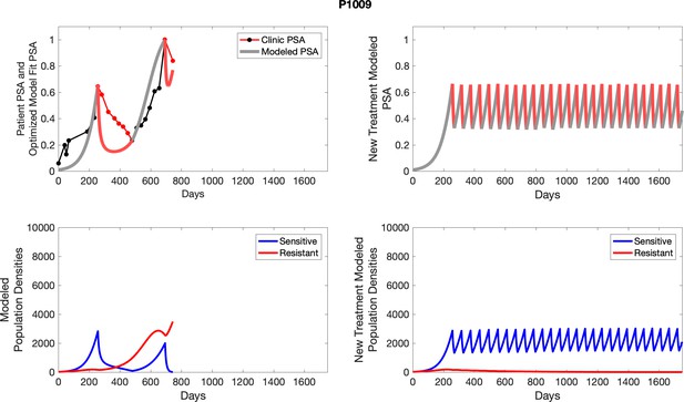
The left column shows actual outcome (upper panel) and computer simulations (lower panel) of the estimated population dynamics of the sensitive and resistant poulations for the indicated subject; the right column shows computer simulations based on an assumption that treatment was stopped immediately when the PSA fell below 0.5 of the pre-treatment and resumed immediately when PSA increased to the pretreatment value.
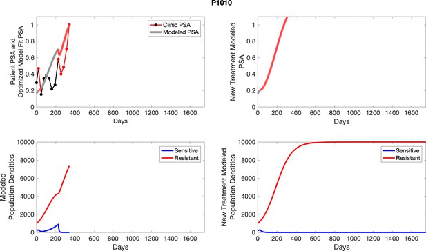
The left column shows actual outcome (upper panel) and computer simulations (lower panel) of the estimated population dynamics of the sensitive and resistant poulations for the indicated subject; the right column shows computer simulations based on an assumption that treatment was stopped immediately when the PSA fell below 0.5 of the pre-treatment and resumed immediately when PSA increased to the pretreatment value.
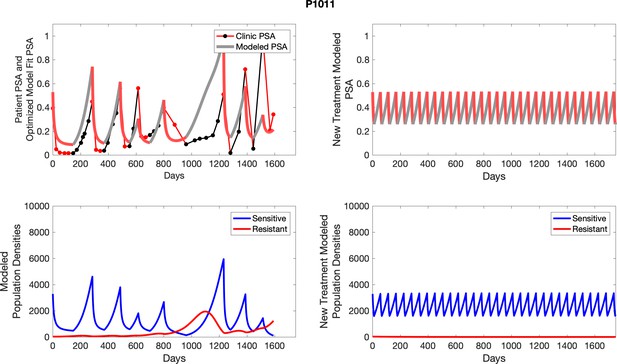
The left column shows actual outcome (upper panel) and computer simulations (lower panel) of the estimated population dynamics of the sensitive and resistant poulations for the indicated subject; the right column shows computer simulations based on an assumption that treatment was stopped immediately when the PSA fell below 0.5 of the pre-treatment and resumed immediately when PSA increased to the pretreatment value.
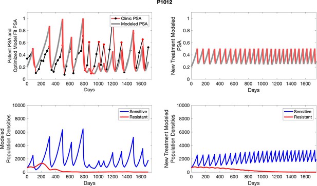
The left column shows actual outcome (upper panel) and computer simulations (lower panel) of the estimated population dynamics of the sensitive and resistant poulations for the indicated subject; the right column shows computer simulations based on an assumption that treatment was stopped immediately when the PSA fell below 0.5 of the pre-treatment and resumed immediately when PSA increased to the pretreatment value.
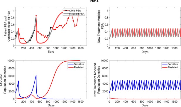
The left column shows actual outcome (upper panel) and computer simulations (lower panel) of the estimated population dynamics of the sensitive and resistant poulations for the indicated subject; the right column shows computer simulations based on an assumption that treatment was stopped immediately when the PSA fell below 0.5 of the pre-treatment and resumed immediately when PSA increased to the pretreatment value.
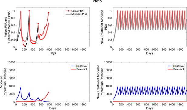
The left column shows actual outcome (upper panel) and computer simulations (lower panel) of the estimated population dynamics of the sensitive and resistant poulations for the indicated subject; the right column shows computer simulations based on an assumption that treatment was stopped immediately when the PSA fell below 0.5 of the pre-treatment and resumed immediately when PSA increased to the pretreatment value.
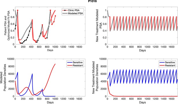
The left column shows actual outcome (upper panel) and computer simulations (lower panel) of the estimated population dynamics of the sensitive and resistant poulations for the indicated subject; the right column shows computer simulations based on an assumption that treatment was stopped immediately when the PSA fell below 0.5 of the pre-treatment and resumed immediately when PSA increased to the pretreatment value.
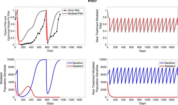
The left column shows actual outcome (upper panel) and computer simulations (lower panel) of the estimated population dynamics of the sensitive and resistant poulations for the indicated subject; the right column shows computer simulations based on an assumption that treatment was stopped immediately when the PSA fell below 0.5 of the pre-treatment and resumed immediately when PSA increased to the pretreatment value.
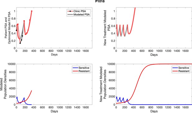
The left column shows actual outcome (upper panel) and computer simulations (lower panel) of the estimated population dynamics of the sensitive and resistant poulations for the indicated subject; the right column shows computer simulations based on an assumption that treatment was stopped immediately when the PSA fell below 0.5 of the pre-treatment and resumed immediately when PSA increased to the pretreatment value.
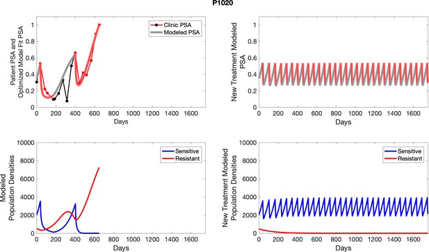
The left column shows actual outcome (upper panel) and computer simulations (lower panel) of the estimated population dynamics of the sensitive and resistant poulations for the indicated subject; the right column shows computer simulations based on an assumption that treatment was stopped immediately when the PSA fell below 0.5 of the pre-treatment and resumed immediately when PSA increased to the pretreatment value.
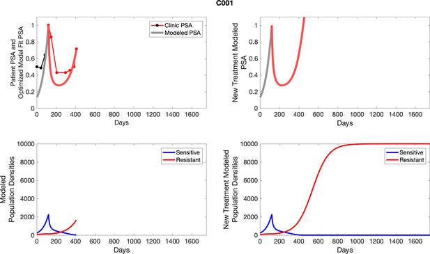
The left column shows actual PSA values (upper right panel) with the PSA dynamics of the fitted mathematical model for the indicated subject, the lower left panel shows computer simulations of the estimated population dynamics for sensitive and resistant cells; the right panels show computer simulations for extended therapy using the standard of care dosing with continuous MTD abiraterone.
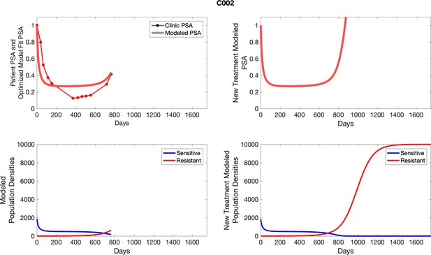
The left column shows actual PSA values (upper right panel) with the PSA dynamics of the fitted mathematical model for the indicated subject, the lower left panel shows computer simulations of the estimated population dynamics for sennsitive and resistant cells; the right panels show computer simulations for extended therapy using the standard of care dosing with continuous MTD abiraterone.
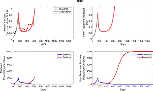
The left column shows actual PSA values (upper right panel) with the PSA dynamics of the fitted mathematical model for the indicated subject, the lower left panel shows computer simulations of the estimated population dynamics for sennsitive and resistant cells; the right panels show computer simulations for extended therapy using the standard of care dosing with continuous MTD abiraterone.
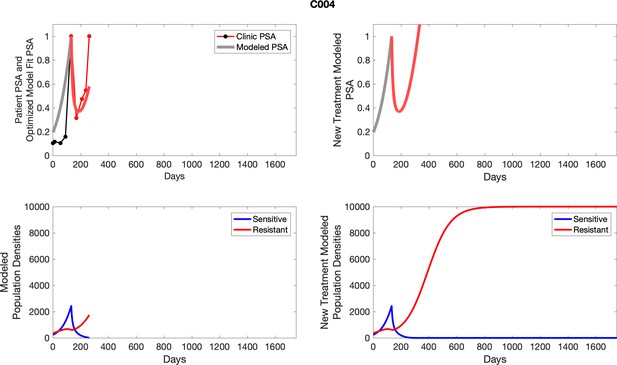
The left column shows actual PSA values (upper right panel) with the PSA dynamics of the fitted mathematical model for the indicated subject, the lower left panel shows computer simulations of the estimated population dynamics for sennsitive and resistant cells; the right panels show computer simulations for extended therapy using the standard of care dosing with continuous MTD abiraterone.

The left column shows actual PSA values (upper right panel) with the PSA dynamics of the fitted mathematical model for the indicated subject, the lower left panel shows computer simulations of the estimated population dynamics for sennsitive and resistant cells; the right panels show computer simulations for extended therapy using the standard of care dosing with continuous MTD abiraterone.
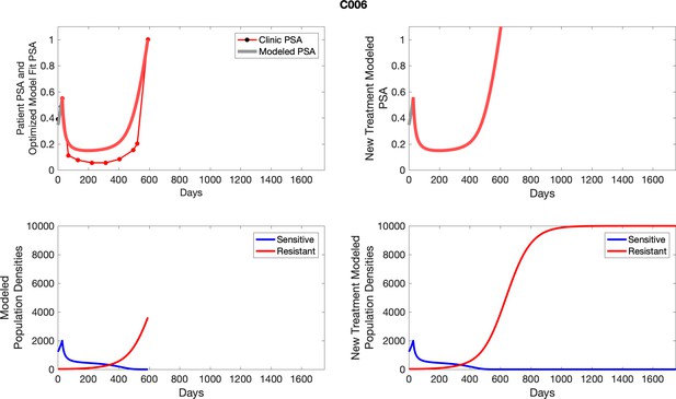
The left column shows actual PSA values (upper right panel) with the PSA dynamics of the fitted mathematical model for the indicated subject, the lower left panel shows computer simulations of the estimated population dynamics for sennsitive and resistant cells; the right panels show computer simulations for extended therapy using the standard of care dosing with continuous MTD abiraterone.
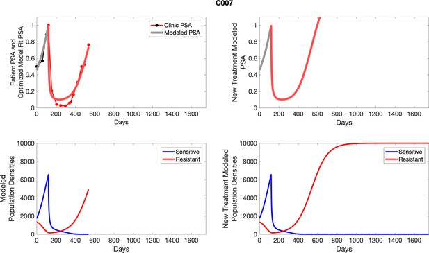
The left column shows actual PSA values (upper right panel) with the PSA dynamics of the fitted mathematical model for the indicated subject, the lower left panel shows computer simulations of the estimated population dynamics for sennsitive and resistant cells; the right panels show computer simulations for extended therapy using the standard of care dosing with continuous MTD abiraterone.
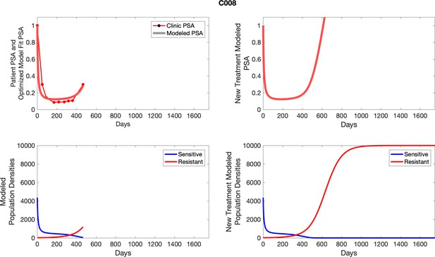
The left column shows actual PSA values (upper right panel) with the PSA dynamics of the fitted mathematical model for the indicated subject, the lower left panel shows computer simulations of the estimated population dynamics for sennsitive and resistant cells; the right panels show computer simulations for extended therapy using the standard of care dosing with continuous MTD abiraterone.

The left column shows actual PSA values (upper right panel) with the PSA dynamics of the fitted mathematical model for the indicated subject, the lower left panel shows computer simulations of the estimated population dynamics for sennsitive and resistant cells; the right panels show computer simulations for extended therapy using the standard of care dosing with continuous MTD abiraterone.
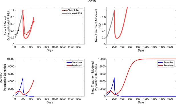
The left column shows actual PSA values (upper right panel) with the PSA dynamics of the fitted mathematical model for the indicated subject, the lower left panel shows computer simulations of the estimated population dynamics for sennsitive and resistant cells; the right panels show computer simulations for extended therapy using the standard of care dosing with continuous MTD abiraterone.
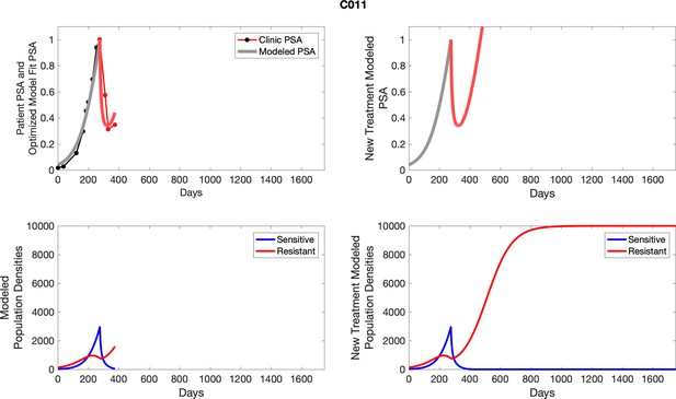
The left column shows actual PSA values (upper right panel) with the PSA dynamics of the fitted mathematical model for the indicated subject, the lower left panel shows computer simulations of the estimated population dynamics for sennsitive and resistant cells; the right panels show computer simulations for extended therapy using the standard of care dosing with continuous MTD abiraterone.
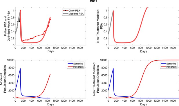
The left column shows actual PSA values (upper right panel) with the PSA dynamics of the fitted mathematical model for the indicated subject, the lower left panel shows computer simulations of the estimated population dynamics for sennsitive and resistant cells; the right panels show computer simulations for extended therapy using the standard of care dosing with continuous MTD abiraterone.
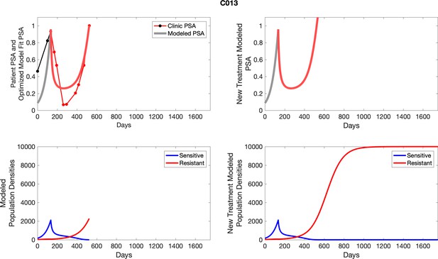
The left column shows actual PSA values (upper right panel) with the PSA dynamics of the fitted mathematical model for the indicated subject, the lower left panel shows computer simulations of the estimated population dynamics for sennsitive and resistant cells; the right panels show computer simulations for extended therapy using the standard of care dosing with continuous MTD abiraterone.
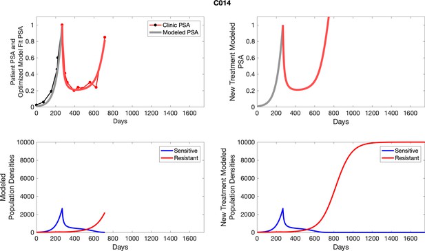
The left column shows actual PSA values (upper right panel) with the PSA dynamics of the fitted mathematical model for the indicated subject, the lower left panel shows computer simulations of the estimated population dynamics for sennsitive and resistant cells; the right panels show computer simulations for extended therapy using the standard of care dosing with continuous MTD abiraterone.

The left column shows actual PSA values (upper right panel) with the PSA dynamics of the fitted mathematical model for the indicated subject, the lower left panel shows computer simulations of the estimated population dynamics for sennsitive and resistant cells; the right panels show computer simulations for extended therapy using the standard of care dosing with continuous MTD abiraterone.
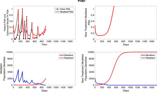
The left column shows actual PSA values (upper right panel) with the PSA dynamics of the fitted mathematical model for the indicated subject, the lower left panel shows computer simulations of the estimated population dynamics for sennsitive and resistant cells; the right panels show computer simulations for extended therapy using the standard of care dosing with continuous MTD abiraterone.
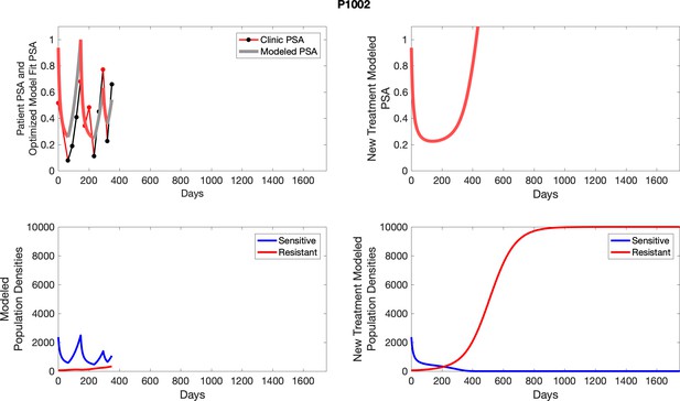
The left column shows actual PSA values (upper right panel) with the PSA dynamics of the fitted mathematical model for the indicated subject, the lower left panel shows computer simulations of the estimated population dynamics for sennsitive and resistant cells; the right panels show computer simulations for extended therapy using the standard of care dosing with continuous MTD abiraterone.
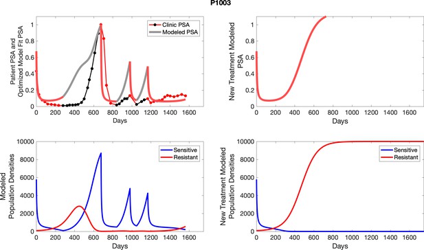
The left column shows actual PSA values (upper right panel) with the PSA dynamics of the fitted mathematical model for the indicated subject, the lower left panel shows computer simulations of the estimated population dynamics for sennsitive and resistant cells; the right panels show computer simulations for extended therapy using the standard of care dosing with continuous MTD abiraterone.
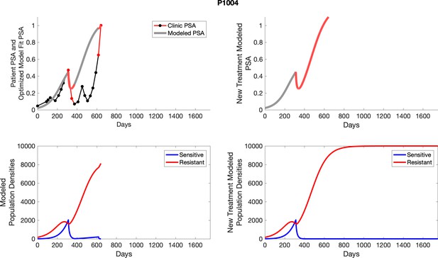
The left column shows actual PSA values (upper right panel) with the PSA dynamics of the fitted mathematical model for the indicated subject, the lower left panel shows computer simulations of the estimated population dynamics for sennsitive and resistant cells; the right panels show computer simulations for extended therapy using the standard of care dosing with continuous MTD abiraterone.
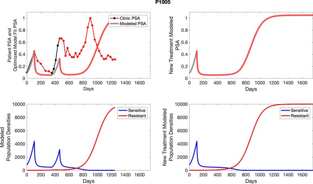
The left column shows actual PSA values (upper right panel) with the PSA dynamics of the fitted mathematical model for the indicated subject, the lower left panel shows computer simulations of the estimated population dynamics for sennsitive and resistant cells; the right panels show computer simulations for extended therapy using the standard of care dosing with continuous MTD abiraterone.

The left column shows actual PSA values (upper right panel) with the PSA dynamics of the fitted mathematical model for the indicated subject, the lower left panel shows computer simulations of the estimated population dynamics for sennsitive and resistant cells; the right panels show computer simulations for extended therapy using the standard of care dosing with continuous MTD abiraterone.
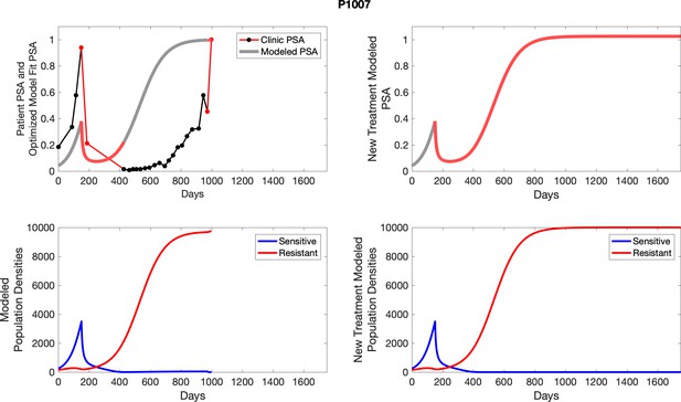
The left column shows actual PSA values (upper right panel) with the PSA dynamics of the fitted mathematical model for the indicated subject, the lower left panel shows computer simulations of the estimated population dynamics for sennsitive and resistant cells; the right panels show computer simulations for extended therapy using the standard of care dosing with continuous MTD abiraterone.
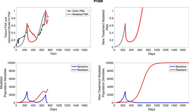
The left column shows actual PSA values (upper right panel) with the PSA dynamics of the fitted mathematical model for the indicated subject, the lower left panel shows computer simulations of the estimated population dynamics for sennsitive and resistant cells; the right panels show computer simulations for extended therapy using the standard of care dosing with continuous MTD abiraterone.
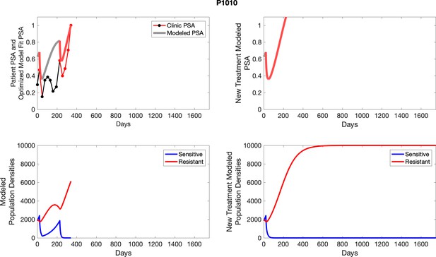
The left column shows actual PSA values (upper right panel) with the PSA dynamics of the fitted mathematical model for the indicated subject, the lower left panel shows computer simulations of the estimated population dynamics for sennsitive and resistant cells; the right panels show computer simulations for extended therapy using the standard of care dosing with continuous MTD abiraterone.
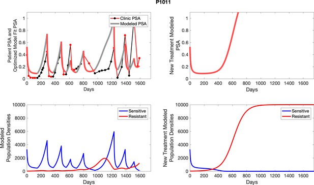
The left column shows actual PSA values (upper right panel) with the PSA dynamics of the fitted mathematical model for the indicated subject, the lower left panel shows computer simulations of the estimated population dynamics for sennsitive and resistant cells; the right panels show computer simulations for extended therapy using the standard of care dosing with continuous MTD abiraterone.

The left column shows actual PSA values (upper right panel) with the PSA dynamics of the fitted mathematical model for the indicated subject, the lower left panel shows computer simulations of the estimated population dynamics for sennsitive and resistant cells; the right panels show computer simulations for extended therapy using the standard of care dosing with continuous MTD abiraterone.
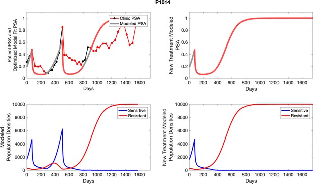
The left column shows actual PSA values (upper right panel) with the PSA dynamics of the fitted mathematical model for the indicated subject, the lower left panel shows computer simulations of the estimated population dynamics for sennsitive and resistant cells; the right panels show computer simulations for extended therapy using the standard of care dosing with continuous MTD abiraterone.
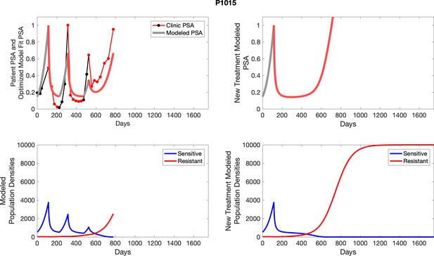
The left column shows actual PSA values (upper right panel) with the PSA dynamics of the fitted mathematical model for the indicated subject, the lower left panel shows computer simulations of the estimated population dynamics for sennsitive and resistant cells; the right panels show computer simulations for extended therapy using the standard of care dosing with continuous MTD abiraterone.

The left column shows actual PSA values (upper right panel) with the PSA dynamics of the fitted mathematical model for the indicated subject, the lower left panel shows computer simulations of the estimated population dynamics for sennsitive and resistant cells; the right panels show computer simulations for extended therapy using the standard of care dosing with continuous MTD abiraterone.
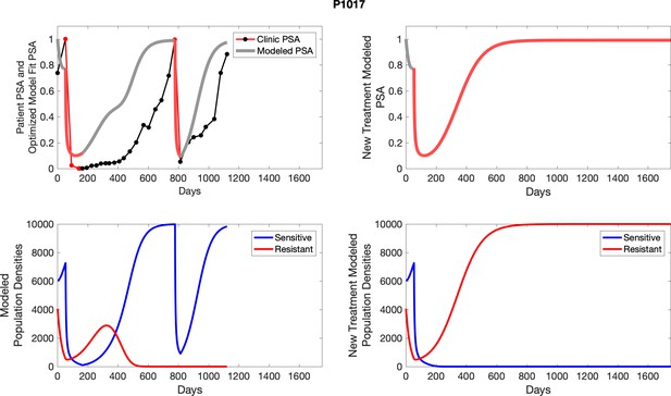
The left column shows actual PSA values (upper right panel) with the PSA dynamics of the fitted mathematical model for the indicated subject, the lower left panel shows computer simulations of the estimated population dynamics for sennsitive and resistant cells; the right panels show computer simulations for extended therapy using the standard of care dosing with continuous MTD abiraterone.

The left column shows actual PSA values (upper right panel) with the PSA dynamics of the fitted mathematical model for the indicated subject, the lower left panel shows computer simulations of the estimated population dynamics for sennsitive and resistant cells; the right panels show computer simulations for extended therapy using the standard of care dosing with continuous MTD abiraterone.

The left column shows actual PSA values (upper right panel) with the PSA dynamics of the fitted mathematical model for the indicated subject, the lower left panel shows computer simulations of the estimated population dynamics for sennsitive and resistant cells; the right panels show computer simulations for extended therapy using the standard of care dosing with continuous MTD abirateron.
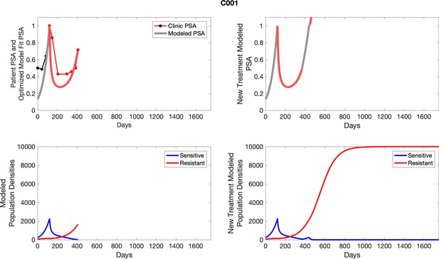
The left column shows PSA changes during treatment and associated model fit for each captioned patient (upper panel) as well as computer simulations for the population dynamics of the resistant and sensitive cells; the right column shows computer simulation in the same patient for a typical “intermittent therapy” protocol in which cycling therapy is insituted only after an 8 month induction period of continuous MTD application of abiraterone.
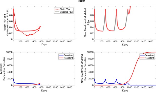
The left column shows PSA changes during treatment and associated model fit for each captioned patient (upper panel) as well as computer simulations for the population dynamics of the resistant and sensitive cells (lower panel); the right column shows computer simulation in the same patient for a typical “intermittent therapy” protocol in which cycling therapy is insituted only after an 8 month induction period of continuous MTD application of abiraterone.
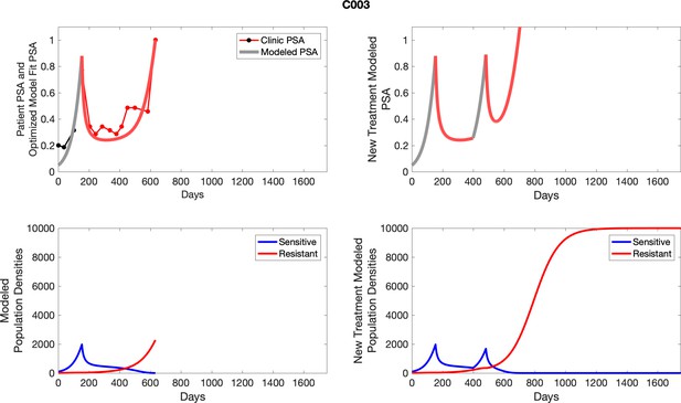
The left column shows PSA changes during treatment and associated model fit for each captioned patient (upper panel) as well as computer simulations for the population dynamics of the resistant and sensitive cells; the right column shows computer simulation in the same patient for a typical “intermittent therapy” protocol in which cycling therapy is insituted only after an 8 month induction period of continuous MTD application of abiraterone.

The left column shows PSA changes during treatment and associated model fit for each captioned patient (upper panel) as well as computer simulations for the population dynamics of the resistant and sensitive cells; the right column shows computer simulation in the same patient for a typical “intermittent therapy” protocol in which cycling therapy is insituted only after an 8 month induction period of continuous MTD application of abiraterone.
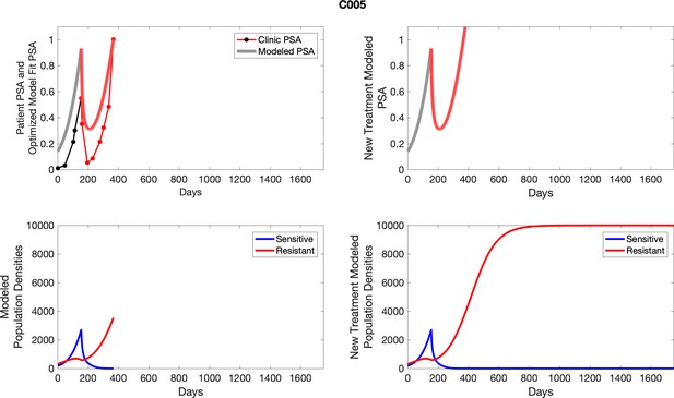
The left column shows PSA changes during treatment and associated model fit for each captioned patient (upper panel) as well as computer simulations for the population dynamics of the resistant and sensitive cells; the right column shows computer simulation in the same patient for a typical “intermittent therapy” protocol in which cycling therapy is insituted only after an 8 month induction period of continuous MTD application of abiraterone.
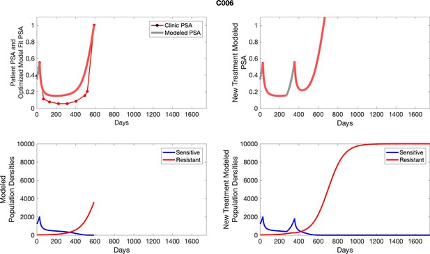
The left column shows PSA changes during treatment and associated model fit for each captioned patient (upper right panel) as well as computer simulations for the population dynamics of the resistant and sensitive cells; the right column shows computer simulation in the same patient for a typical “intermittent therapy” protocol in which cycling therapy is insituted only after an 8 month induction period of continuous MTD application of abiraterone.
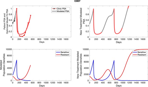
The left column shows PSA changes during treatment and associated model fit for each captioned patient (upper panel) as well as computer simulations for the population dynamics of the resistant and sensitive cells; the right column shows computer simulation in the same patient for a typical “intermittent therapy” protocol in which cycling therapy is insituted only after an 8 month induction period of continuous MTD application of abiraterone.
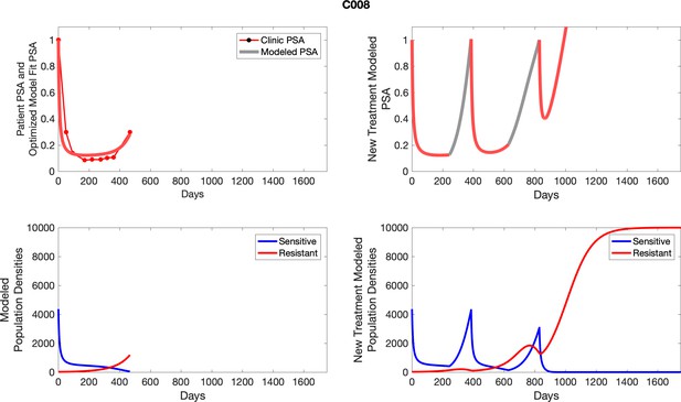
The left column shows PSA changes during treatment and associated model fit for each captioned patient (upper panel) as well as computer simulations for the population dynamics of the resistant and sensitive cells; the right column shows computer simulation in the same patient for a typical “intermittent therapy” protocol in which cycling therapy is insituted only after an 8 month induction period of continuous MTD application of abiraterone.

The left column shows PSA changes during treatment and associated model fit for each captioned patient (upper panel) as well as computer simulations for the population dynamics of the resistant and sensitive cells; the right column shows computer simulation in the same patient for a typical “intermittent therapy” protocol in which cycling therapy is insituted only after an 8 month induction period of continuous MTD application of abiraterone.
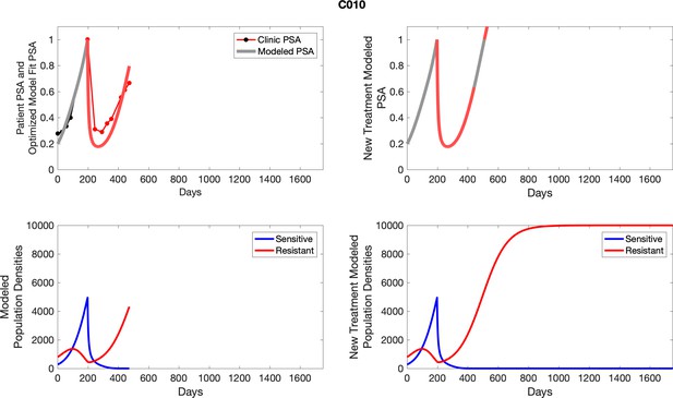
The left column shows PSA changes during treatment and associated model fit for each captioned patient (upper panel) as well as computer simulations for the population dynamics of the resistant and sensitive cells; the right column shows computer simulation in the same patient for a typical “intermittent therapy” protocol in which cycling therapy is insituted only after an 8 month induction period of continuous MTD application of abiraterone.

The left column shows PSA changes during treatment and associated model fit for each captioned patient (upper panel) as well as computer simulations for the population dynamics of the resistant and sensitive cells; the right column shows computer simulation in the same patient for a typical “intermittent therapy” protocol in which cycling therapy is insituted only after an 8 month induction period of continuous MTD application of abiraterone.
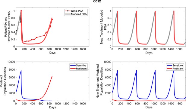
The left column shows PSA changes during treatment and associated model fit for each captioned patient (upper panel) as well as computer simulations for the population dynamics of the resistant and sensitive cells; the right column shows computer simulation in the same patient for a typical “intermittent therapy” protocol in which cycling therapy is insituted only after an 8 month induction period of continuous MTD application of abiraterone.
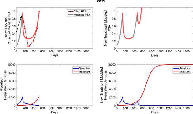
The left column shows PSA changes during treatment and associated model fit for each captioned patient (upper panel) as well as computer simulations for the population dynamics of the resistant and sensitive cells; the right column shows computer simulation in the same patient for a typical “intermittent therapy” protocol in which cycling therapy is insituted only after an 8 month induction period of continuous MTD application of abiraterone.
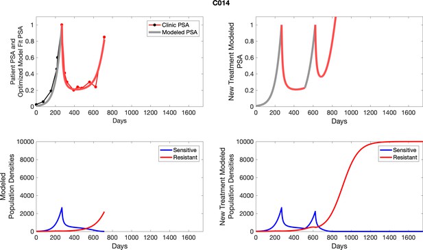
The left column shows PSA changes during treatment and associated model fit for each captioned patient (upper right panel) as well as computer simulations for the population dynamics of the resistant and sensitive cells; the right column shows computer simulation in the same patient for a typical “intermittent therapy” protocol in which cycling therapy is insituted only after an 8 month induction period of continuous MTD application of abiraterone.
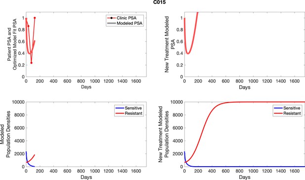
The left column shows PSA changes during treatment and associated model fit for each captioned patient (upper panel) as well as computer simulations for the population dynamics of the resistant and sensitive cells; the right column shows computer simulation in the same patient for a typical “intermittent therapy” protocol in which cycling therapy is insituted only after an 8 month induction period of continuous MTD application of abiraterone.
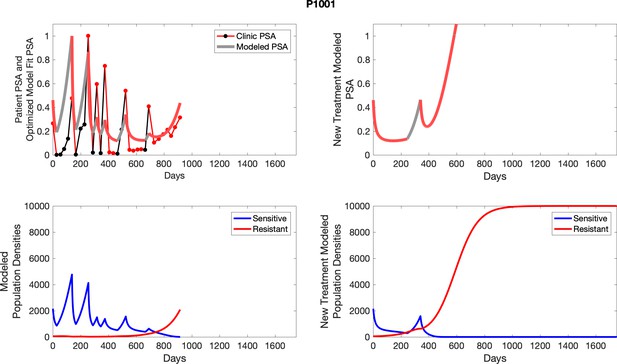
The left column shows PSA changes during treatment and associated model fit for each captioned patient (upper panel) as well as computer simulations for the population dynamics of the resistant and sensitive cells; the right column shows computer simulation in the same patient for a typical “intermittent therapy” protocol in which cycling therapy is insituted only after an 8 month induction period of continuous MTD application of abiraterone.
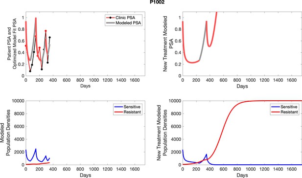
The left column shows PSA changes during treatment and associated model fit for each captioned patient (upper panel) as well as computer simulations for the population dynamics of the resistant and sensitive cells; the right column shows computer simulation in the same patient for a typical “intermittent therapy” protocol in which cycling therapy is insituted only after an 8 month induction period of continuous MTD application of abiraterone.
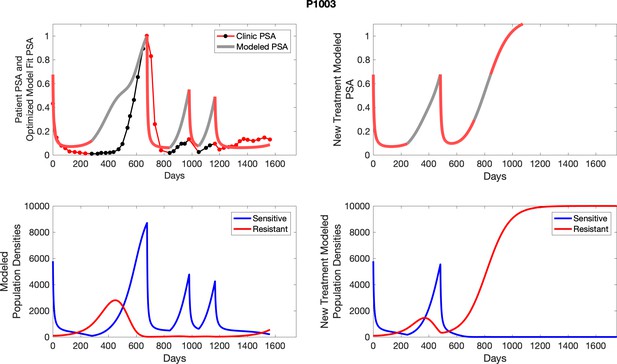
The left column shows PSA changes during treatment and associated model fit for each captioned patient (upper panel) as well as computer simulations for the population dynamics of the resistant and sensitive cells; the right column shows computer simulation in the same patient for a typical “intermittent therapy” protocol in which cycling therapy is insituted only after an 8 month induction period of continuous MTD application of abiraterone.
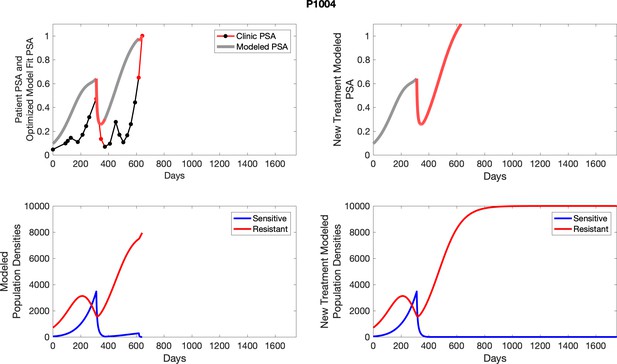
The left column shows PSA changes during treatment and associated model fit for each captioned patient (upper panel) as well as computer simulations for the population dynamics of the resistant and sensitive cells; the right column shows computer simulation in the same patient for a typical “intermittent therapy” protocol in which cycling therapy is insituted only after an 8 month induction period of continuous MTD application of abiraterone.
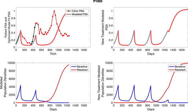
The left column shows PSA changes during treatment and associated model fit for each captioned patient (upper panel) as well as computer simulations for the population dynamics of the resistant and sensitive cells; the right column shows computer simulation in the same patient for a typical “intermittent therapy” protocol in which cycling therapy is insituted only after an 8 month induction period of continuous MTD application of abiraterone.
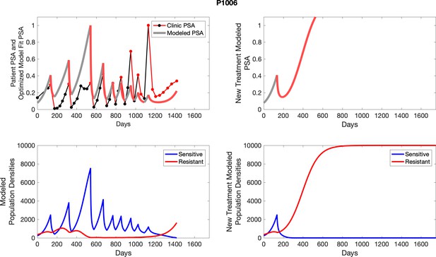
The left column shows PSA changes during treatment and associated model fit for each captioned patient (upper panel) as well as computer simulations for the population dynamics of the resistant and sensitive cells; the right column shows computer simulation in the same patient for a typical “intermittent therapy” protocol in which cycling therapy is insituted only after an 8 month induction period of continuous MTD application of abiraterone.
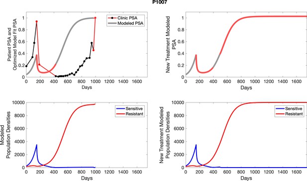
The left column shows PSA changes during treatment and associated model fit for each captioned patient (upper panel) as well as computer simulations for the population dynamics of the resistant and sensitive cells; the right column shows computer simulation in the same patient for a typical “intermittent therapy” protocol in which cycling therapy is insituted only after an 8 month induction period of continuous MTD application of abiraterone.
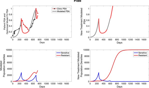
The left column shows PSA changes during treatment and associated model fit for each captioned patient (upper panel) as well as computer simulations for the population dynamics of the resistant and sensitive cells; the right column shows computer simulation in the same patient for a typical “intermittent therapy” protocol in which cycling therapy is insituted only after an 8 month induction period of continuous MTD application of abiraterone.

The left column shows PSA changes during treatment and associated model fit for each captioned patient (upper panel) as well as computer simulations for the population dynamics of the resistant and sensitive cells; the right column shows computer simulation in the same patient for a typical “intermittent therapy” protocol in which cycling therapy is insituted only after an 8 month induction period of continuous MTD application of abiraterone.
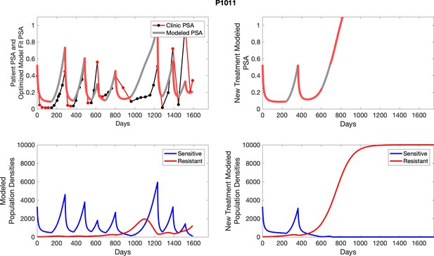
The left column shows PSA changes during treatment and associated model fit for each captioned patient (upper panel) as well as computer simulations for the population dynamics of the resistant and sensitive cells; the right column shows computer simulation in the same patient for a typical “intermittent therapy” protocol in which cycling therapy is insituted only after an 8 month induction period of continuous MTD application of abiraterone.
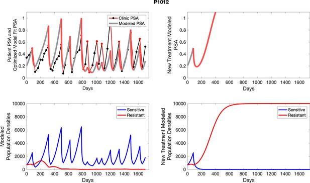
The left column shows PSA changes during treatment and associated model fit for each captioned patient (upper panel) as well as computer simulations for the population dynamics of the resistant and sensitive cells; the right column shows computer simulation in the same patient for a typical “intermittent therapy” protocol in which cycling therapy is insituted only after an 8 month induction period of continuous MTD application of abiraterone.
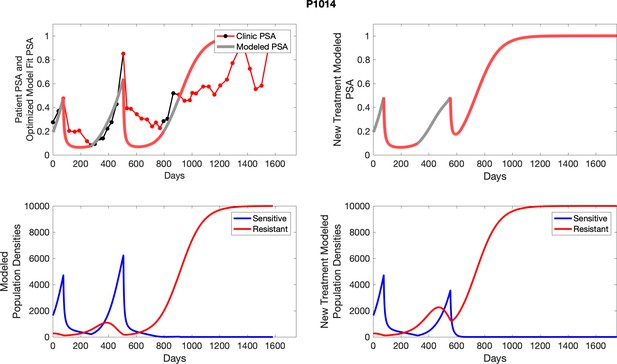
The left column shows PSA changes during treatment and associated model fit for each captioned patient (upper panel) as well as computer simulations for the population dynamics of the resistant and sensitive cells; the right column shows computer simulation in the same patient for a typical “intermittent therapy” protocol in which cycling therapy is insituted only after an 8 month induction period of continuous MTD application of abiraterone.
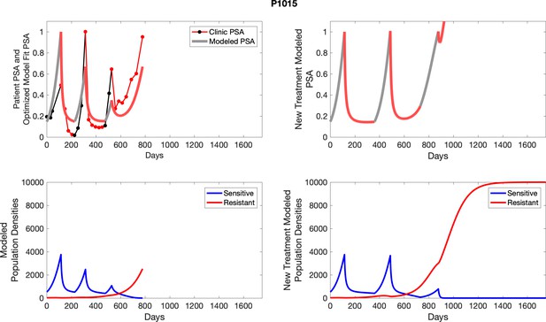
The left column shows PSA changes during treatment and associated model fit for each captioned patient (upper panel) as well as computer simulations for the population dynamics of the resistant and sensitive cells; the right column shows computer simulation in the same patient for a typical “intermittent therapy” protocol in which cycling therapy is insituted only after an 8 month induction period of continuous MTD application of abiraterone.
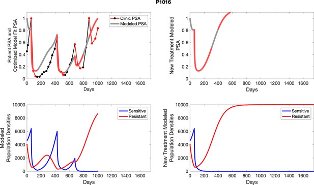
The left column shows PSA changes during treatment and associated model fit for each captioned patient (upper right panel) as well as computer simulations for the population dynamics of the resistant and sensitive cells; the right column shows computer simulation in the same patient for a typical “intermittent therapy” protocol in which cycling therapy is insituted only after an 8 month induction period of continuous MTD application of abiraterone.
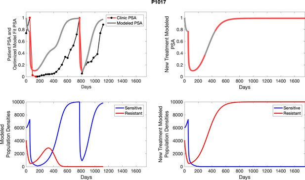
The left column shows PSA changes during treatment and associated model fit for each captioned patient (upper panel) as well as computer simulations for the population dynamics of the resistant and sensitive cells; the right column shows computer simulation in the same patient for a typical “intermittent therapy” protocol in which cycling therapy is insituted only after an 8 month induction period of continuous MTD application of abiraterone.
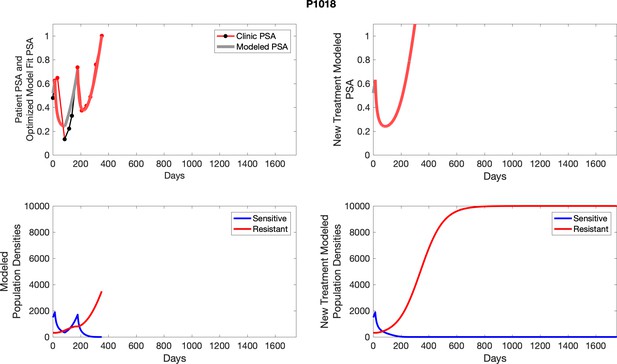
The left column shows PSA changes during treatment and associated model fit for each captioned patient (upper panel) as well as computer simulations for the population dynamics of the resistant and sensitive cells; the right column shows computer simulation in the same patient for a typical “intermittent therapy” protocol in which cycling therapy is insituted only after an 8 month induction period of continuous MTD application of abiraterone.
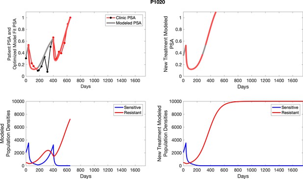
The left column shows PSA changes during treatment and associated model fit for each captioned patient (upper panel) as well as computer simulations for the population dynamics of the resistant and sensitive cells; the right column shows computer simulation in the same patient for a typical “intermittent therapy” protocol in which cycling therapy is insituted only after an 8 month induction period of continuous MTD application of abiraterone.
Tables
Demographic and prior treatment history in each cohort.
The study was conducted before abiraterone, enzalutamide, or apalutamide was approved for treating castration-sensitive prostate cancer. Sipuleucel-T was the only treatment given before abiraterone for metastatic castrate-resistant prostate cancer (mCRPC) in the control and adaptive abiraterone cohorts.
| Control (Pfister, 1995) | Adaptive abiraterone (Zhang et al., 2017) | |
|---|---|---|
| Age/mean [range] | 68 [57–76] | 67 [50–79] |
| History of androgen deprivation therapy for M0 prostate cancer | 5 | 7 |
| <12 months of androgen deprivation therapy prior to abiraterone for mCRPC | 3 | 3 |
| Sipuleucel-T prior to abiraterone | 5 | 6 |
| Gleason score/median [range] | 7 [7, 10] | 8 [6, 10] |
| Pre-abiraterone PSA/mean [range] | 36.52 [2.71, 93.4] | 29.7 [1.46, 109.4] |
| Lymph node metastases only | 1 | 1 |
| Bone, with or without lymph node metastases | 14 | 15 |
| Lung or soft tissue metastases | 1 | 1 |
Estimates of sensitive, resistant growth rates from patient data in both the contemporaneous and adaptive therapy cohorts.
| Sensitive cells | Resistant cells | ||
|---|---|---|---|
| Patient identifier | Extracted growth rate | Patient identifier | Extracted growth rate |
| C010 | 0.0071 | C013 | 0.0109 |
| C014 | 0.0142 | C012 | 0.0025 |
| C012 | 0.0075 | C010 | 0.0046 |
| C011 | 0.0123 | C005 | 0.0173 |
| C009 | 0.0107 | C008 | 0.0047 |
| C007 | 0.0062 | C007 | 0.0111 |
| C005 | 0.0214 | C006 | 0.0130 |
| C004 | 0.0196 | C005 | 0.0173 |
| C003 | 0.0100 | C004 | 0.0124 |
| C001 | 0.0062 | C002 | 0.0031 |
| P1018 | 0.0189 | C001 | 0.0022 |
| P1017 | 0.0068 | ||
| P1016 | 0.0106 | ||
| P1016 | 0.0146 | ||
| P1015 | 0.0419 | ||
| P1014 | 0.0109 | ||
| P1012 | 0.0059 | ||
| P1012 | 0.0076 | ||
| P1012 | 0.0091 | ||
| P1012 | 0.0160 | ||
| P1012 | 0.0100 | ||
| P1012 | 0.0170 | ||
| P1011 | 0.0191 | ||
| P1011 | 0.0191 | ||
| P1011 | 0.0304 | ||
| P1007 | 0.0118 | ||
| P1006 | 0.0216 | ||
| P1004 | 0.0071 | ||
| P1003 | 0.0124 | ||
| P1003 | 0.0116 | ||
| P1003 | 0.0105 | ||
| P1002 | 0.0245 | ||
| P1001 | 0.0446 | ||
| P1001 | 0.0317 | ||
Table of parameters and definitions to be optimized using constrained optimization.
| Parameter | Definition |
|---|---|
| Abundance of sensitive cells at the time of initial treatment | |
| Abundance of resistant cells at the time of initial treatment | |
| Competitive effect of sensitive cells on resistant cells | |
| Ecological scale factor |
Table of constraints on parameters to be optimized using constrained optimization.
| Parameter | Constraint |
|---|---|
Optimized parameters for each patient resulting from nonlinear constrained optimization.
| Patient | ||||
|---|---|---|---|---|
| P1001 | 86.74 | 1.00 | 6 | 8 |
| P1002 | 165.99 | 24.67 | 6 | 8 |
| P1003 | 10000.00 | 124.98 | 6 | 8 |
| P1004 | 19.90 | 400.57 | 6 | 8 |
| P1005 | 802.20 | 12.31 | 6 | 8 |
| P1006 | 102.28 | 174.59 | 6 | 8 |
| P1007 | 253.07 | 149.12 | 6 | 8 |
| P1009 | 20.41 | 23.61 | 6 | 8 |
| P1010 | 196.09 | 1001.19 | 6 | 8 |
| P1011 | 29.19 | 6.31 | 6 | 8 |
| P1012 | 567.60 | 663.13 | 6 | 8 |
| P1014 | 1640.76 | 273.61 | 6 | 8 |
| P1015 | 126.13 | 6.38 | 6 | 8 |
| P1016 | 4589.21 | 4078.11 | 6 | 8 |
| P1017 | 6035.16 | 4060.25 | 6 | 8 |
| P1018 | 1495.72 | 318.18 | 6 | 8 |
| P1020 | 2061.34 | 477.07 | 6 | 8 |
| C001 | 111.70 | 19.46 | 6 | 8 |
| C002 | 1867.68 | 1.00 | 6 | 8 |
| C003 | 61.96 | 5.81 | 6 | 8 |
| C004 | 110.57 | 156.36 | 6 | 8 |
| C005 | 66.07 | 127.48 | 6 | 8 |
| C006 | 1226.45 | 25.31 | 6 | 8 |
| C007 | 1740.08 | 1325.03 | 6 | 8 |
| C008 | 4362.58 | 24.08 | 6 | 8 |
| C009 | 148.30 | 936.54 | 6 | 8 |
| C010 | 273.95 | 798.61 | 6 | 8 |
| C011 | 19.85 | 129.22 | 6 | 8 |
| C012 | 2148.71 | 301.47 | 6 | 8 |
| C013 | 165.20 | 31.48 | 6 | 8 |
| C014 | 13.57 | 5.09 | 6 | 8 |
| C015 | 1211.43 | 483.69 | 6 | 8 |
Tumor composition of sensitive and resistant populations at the time of initial abiraterone therapy from the optimized model fits to patient data.
The calculated percentage of resistant to sensitive cells alongside the clinical time to progression (TTP) for each patient is also shown.
| Patient | % | TTP | ||
|---|---|---|---|---|
| P1001 | 2158.32 | 52.35 | 2.43 | 30.6 |
| P1003 | 5782.98 | 105.32 | 1.82 | 53.1 |
| P1004 | 3475.70 | 1621.81 | 46.66 | 11.0 |
| P1005 | 4407.49 | 7.77 | 0.18 | 38.0 |
| P1006 | 2483.02 | 603.80 | 24.32 | 42.8 |
| P1007 | 3503.41 | 203.61 | 5.81 | 30.1 |
| P1009 | 2830.43 | 156.89 | 5.54 | 17.0 |
| P1010 | 2407.93 | 1765.24 | 73.31 | 10.7 |
| P1011 | 3285.31 | 26.37 | 0.80 | 25.4 |
| P1012 | 2530.65 | 706.23 | 27.91 | 54.0 |
| P1014 | 4708.02 | 127.91 | 2.72 | 50.0 |
| P1015 | 3757.24 | 23.55 | 0.63 | 20.4 |
| P1016 | 6418.04 | 678.74 | 10.58 | 31.4 |
| P1017 | 7268.07 | 557.30 | 7.67 | 35.5 |
| P1018 | 1887.88 | 315.85 | 16.73 | 10.8 |
| P1020 | 3534.42 | 346.12 | 9.79 | 23.0 |
| C001 | 2250.42 | 136.14 | 6.05 | 9.0 |
| C002 | 1867.68 | 1.00 | 0.05 | 26.0 |
| C003 | 1976.15 | 32.96 | 1.67 | 15.0 |
| C004 | 2435.97 | 617.06 | 25.33 | 4.2 |
| C005 | 2696.58 | 600.39 | 22.26 | 7.0 |
| C006 | 1998.86 | 25.70 | 1.29 | 17.7 |
| C007 | 6552.52 | 166.29 | 2.54 | 17.3 |
| C008 | 4362.58 | 24.08 | 0.55 | 19.6 |
| C009 | 4545.92 | 787.31 | 17.32 | 6.5 |
| C010 | 4951.79 | 472.52 | 9.54 | 9.0 |
| C011 | 2953.60 | 772.31 | 26.15 | 4.0 |
| C012 | 7754.85 | 15.28 | 0.20 | 25.0 |
| C013 | 2113.11 | 72.78 | 3.44 | 13.8 |
| C014 | 2645.67 | 44.98 | 1.70 | 14.8 |
| C015 | 2356.24 | 683.69 | 29.02 | 3.2 |


