Nomograms of human hippocampal volume shifted by polygenic scores
- Centre for Medical Image Computing (CMIC), Department of Medical Physics and Biomedical Engineering, University College London, United Kingdom
- Medical and Population Genomics Lab, Human Genetics Department, Research Branch, Sidra Medicine, Qatar
- Stevens Neuroimaging and Informatics Institute, Keck School of Medicine, University of Southern California, United States
- Dementia Research Centre (DRC), Queen Square Institute of Neurology, University College London, United Kingdom
- Department of Genetic Medicine, Weill Cornell Medicine-Qatar, Qatar
Figures
Figure 1
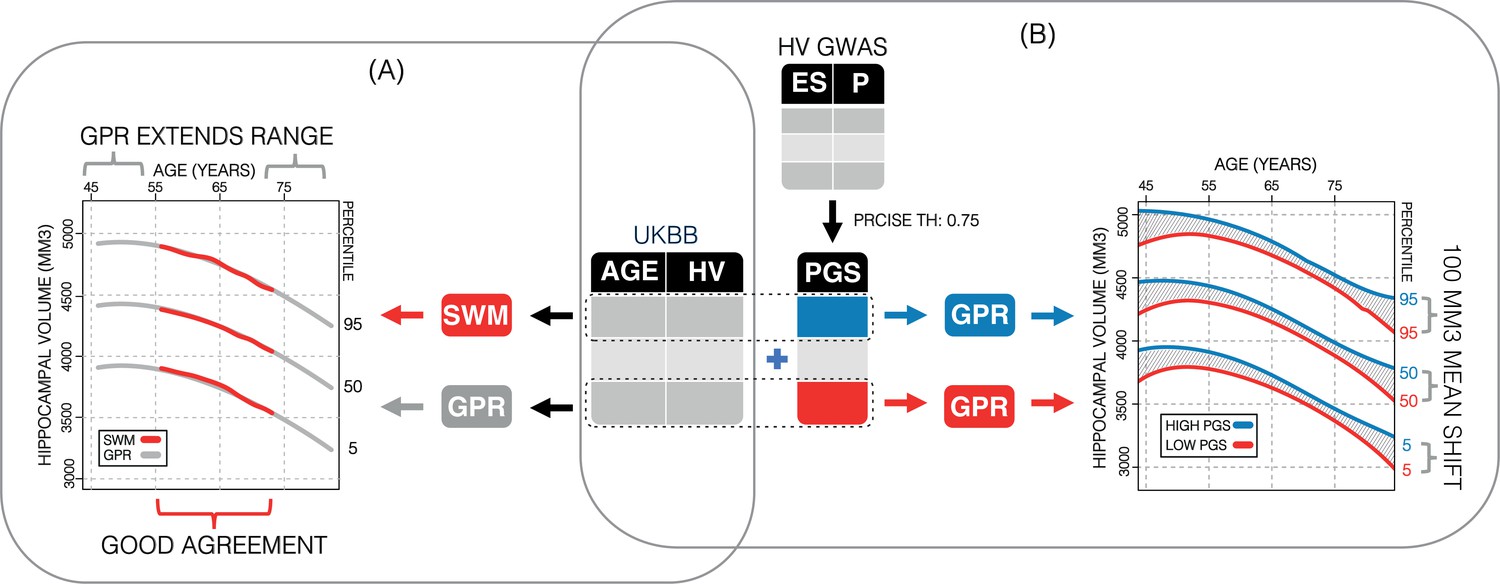
Study overview.
(A) Using 35,686 subjects from the UK Biobank, we generate nomograms using two methods: a previously reported sliding window method (SWM) and Gaussian process regression (GPR). We find that GPR is more data efficient than the SWM and can extend the nomogram into dementia critical age ranges. (B) Using a previously reported genome-wide association study, we generate polygenic scores (PGSs) for the subjects in our UK Biobank table. We then stratify the table by PGS and generate nomograms for the top and bottom 30% of samples separately. We find the genetic adjustment differentiates the nomograms by an average of 100 mm3, which is equivalent to about 3 years of normal aging for a 65-year-old.
Figure 2 with 4 supplements
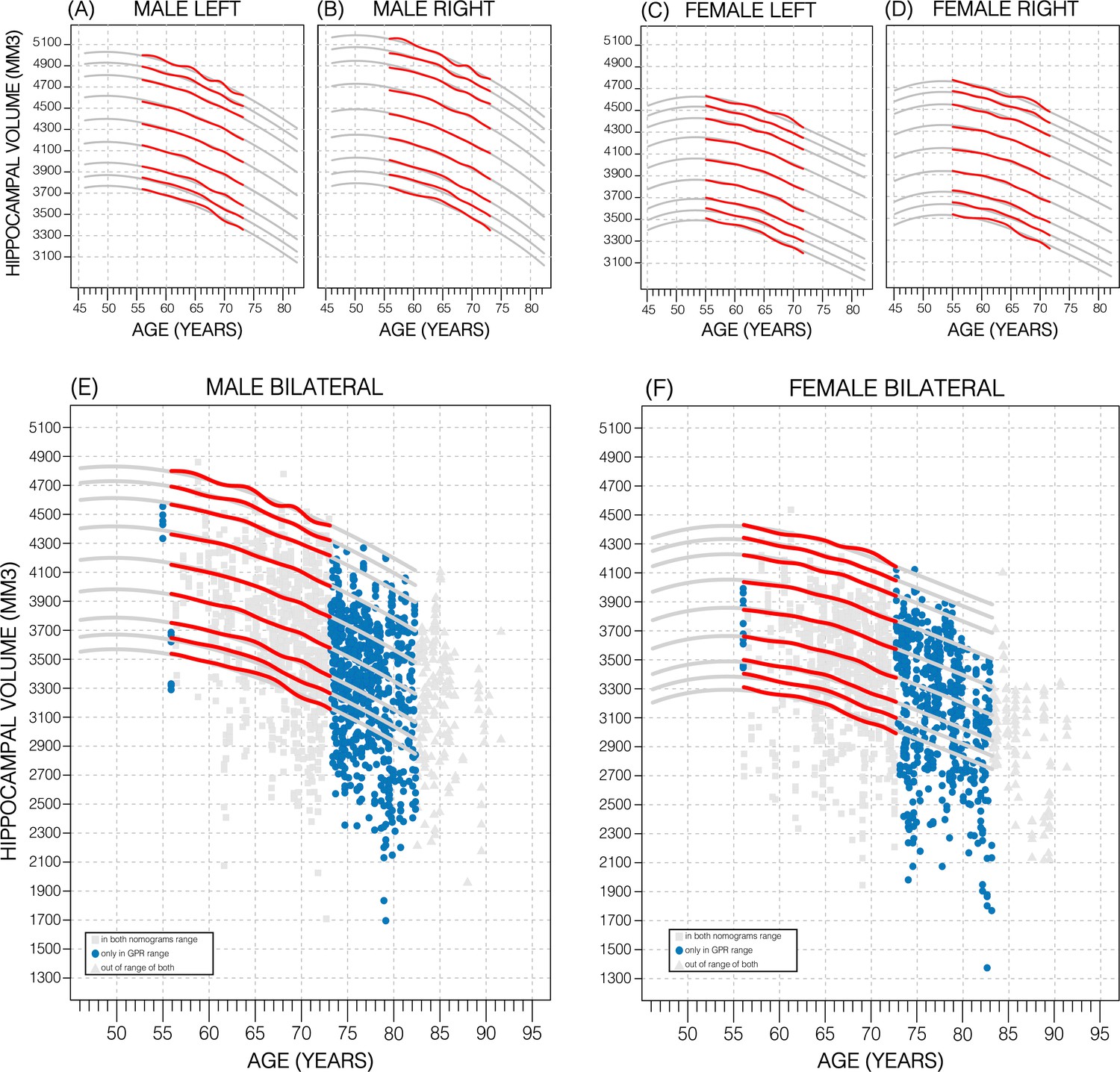
Comparing nomogram generation methods.
Nomograms produced from healthy UK Biobank (UKB) subjects using the sliding window approach (SWA) (red lines) and Gaussian process regression (GPR) method (grey lines) show similar trends. Both left hemisphere nomograms (A, C) are lower than their right counterparts (B, D). Male nomograms are higher than female nomograms (A vs. C) and (B vs. D). Female hippocampal volume (HV) shows a peak at 53.5 years of age, while male HV shows a less prominent peak at 50 years of age. SWA and GPR show good agreement, while GPR enables a 10-year nomogram extension in either direction. The benefits of this extension can be seen with scatter plots of Alzheimer’s Disease Neuroimaging Initiative (ADNI) subjects of all diagnoses overlayed (E, F). The extended age range of the GPR nomograms (45–82 years) enables the evaluation of an additional 43% of male data (E) and 34% of female data (F) (turquoise circles). A similar figure with only the cognitively normal ADNI subjects can be found in Figure 2—figure supplement 2.
Figure 2—figure supplement 1
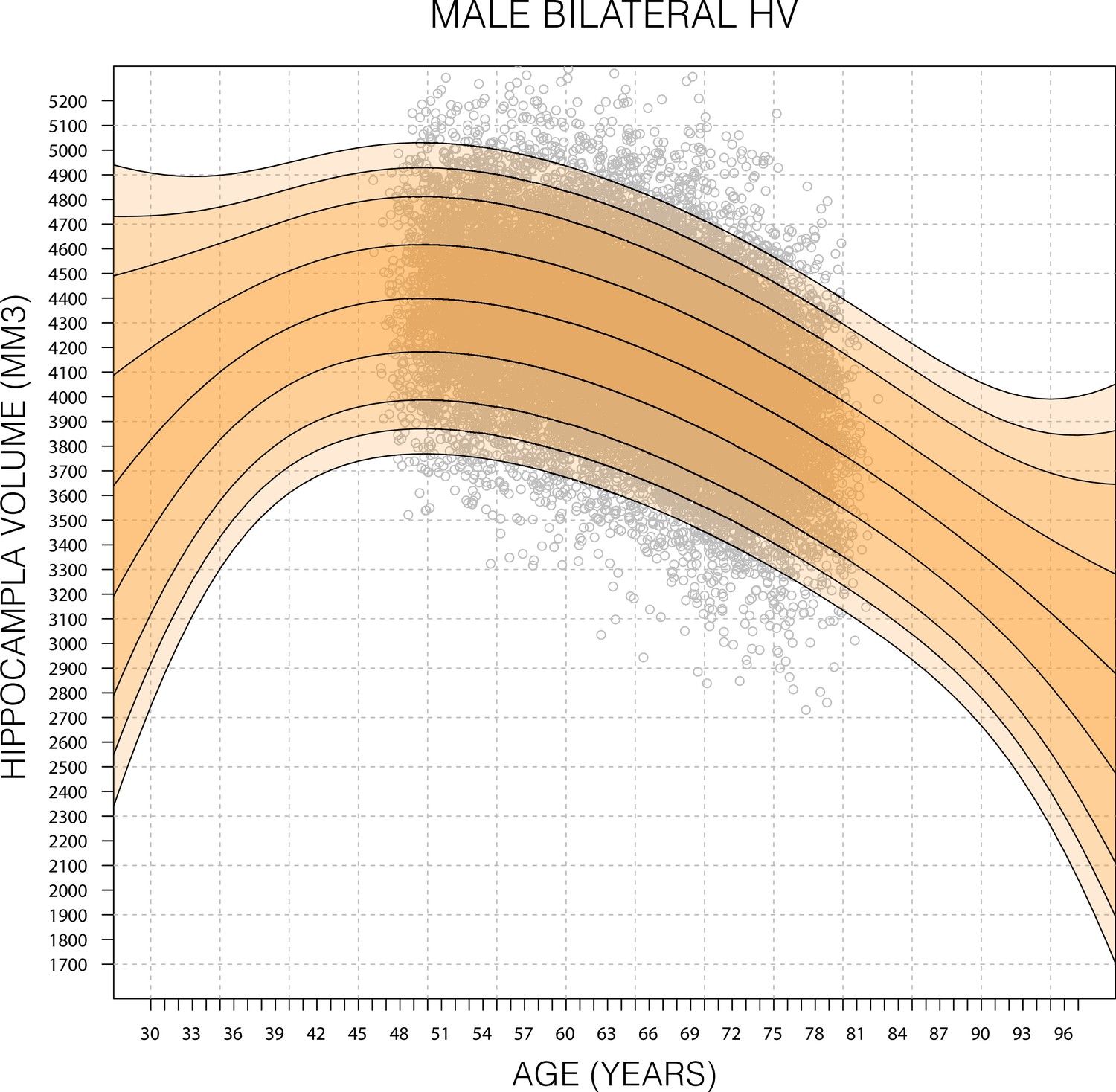
Expanded Gaussian process regression (GPR) nomogram.
A GPR model trained with mean bilateral hippocampal volume (HV) of male subjects in the age range 45–82 (grey circles) and then generated nomograms for the age range 30–100. Within training data range nomogram follows data reasonably well. Outside data rage, nomogram flairs out from expected range after 2–6 years. Fairing is faster in the lower ages because, outside the data range, the GPR model reverts to a normal distribution with zero mean. For all sub-figures, the black lines – from top to bottom – represent the 2.5%, 5%, 10%, 25%, 50%, 75%, 90%, 95%, and 97.5% quantiles, respectively.
Figure 2—figure supplement 2
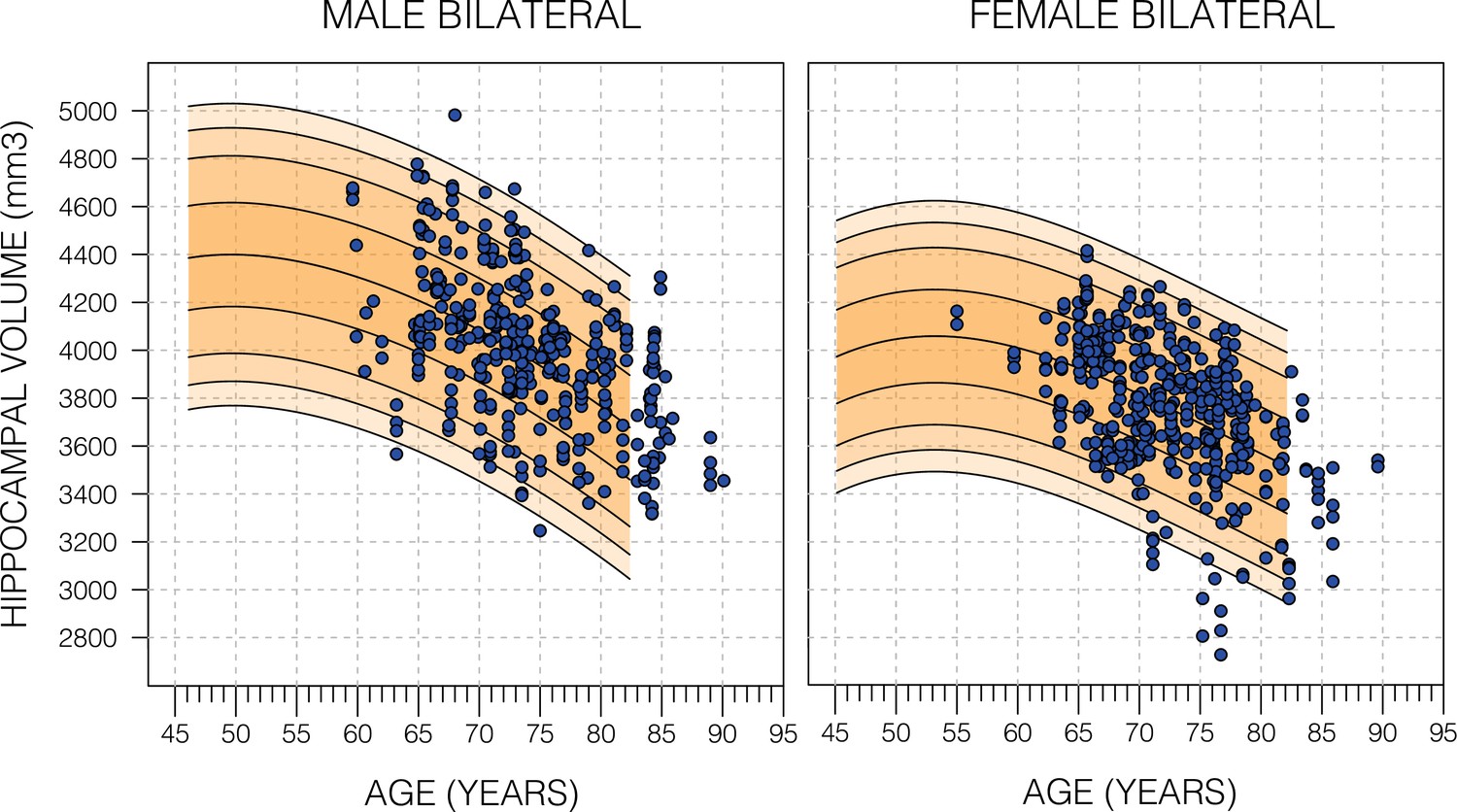
Model fit of healthy Alzheimer’s Disease Neuroimaging Initiative (ADNI) subjects.
Nomograms produced from healthy subjects in the UK Biobank (UKB) using the Gaussian process regression (GPR) method. Overlayed are scatter plots cognitively normal subjects from the ADNI dataset. Male subjects averaged (56.9%±24.6 SD) and female subjects averaged (54.9±26.5 SD). For both sub-figures, the black lines – from top to bottom – represent the 2.5%, 5%, 10%, 25%, 50%, 75%, 90%, 95%, and 97.5% quantiles respectively.
Figure 2—figure supplement 3
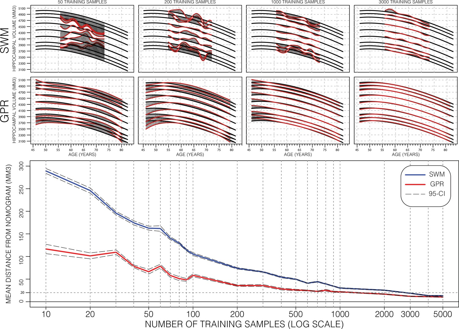
Performance of Gaussian process regression (GPR) and sliding window method (SWM) across sample size.
Model training progression is shown for both SWM (top row) and GPR (middle row) models at representative training sizes. Performance (bottom figure) is summarized using the mean distance between generated nomograms and the GPR nomograms built with the full training set (~15k) (shaded areas in the top two rows). By repeatedly sampling data from across age (10 times at each training sample size), we plot the average performance and 95% CI of each method. Both methods are data efficient, SWM can achieve 20 mm3 mean difference (0.4% of mean hippocampal volume [HV]) performance using ~3000 samples (20% of training set), and GPR can achieve the same performance using only 1000 samples (~7% of training set).
Figure 2—figure supplement 4
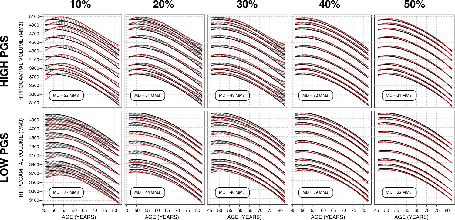
Gaussian process regression (GPR) model across top/bottom thresholds.
Illustrated is male bilateral hippocampal volume (HV). When stratifying by polygenic risk score (PRS), there is a trade-off between training set size and final model performance. In these figures, performance is measured by average distance between the percentile curves. At 10%, (leftmost column), the top/bottom strata contain ~1500 samples each and the mean distance is 65 mm3, and at 50% (the rightmost column) they contain ~7500 and the mean distance is 21.5 mm3. For all sub-figures, the black lines – from top to bottom – represent the 2.5%, 5%, 10%, 25%, 50%, 75%, 90%, 95%, and 97.5% quantiles, respectively.
Figure 3 with 2 supplements
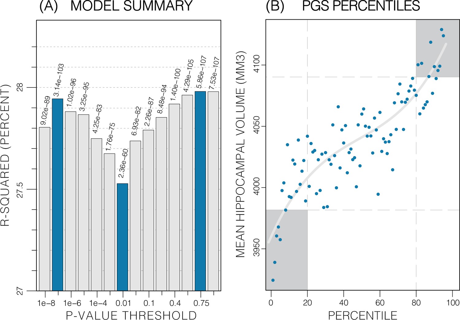
Summary of polygenic score (PGS) models.
Polygenic risk score in models of mean hippocampal volume (HV) across both sexes. (A) R2 of linear models across increasing p-value thresholds. All models are of bilateral HV and account for age, sex, and top 10 genetic principal components. The minimum R2 on the y-scale is the R2 of the models without any PGS. (B) Distribution of mean HV across percentiles of PGS. Excluding the top and bottom 20% of percentiles reduces the variance by 49% (darker grey areas). Fitting a cubic polynomial to the means produces the grey line.
-
Figure 3—source data 1
Summary of PGS vs HV regression models.
- https://cdn.elifesciences.org/articles/78232/elife-78232-fig3-data1-v2.xlsx
Figure 3—figure supplement 1
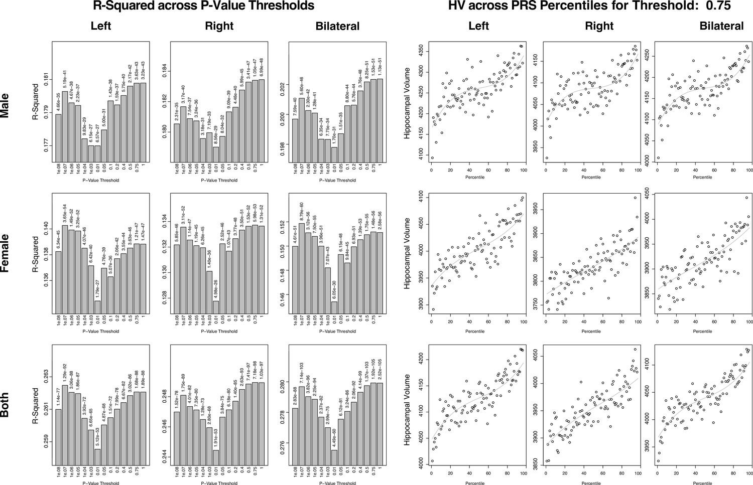
Summary of polygenic scores (PGSs) based on hippocampal volume (HV) genome-wide association study (GWAS) in UK Biobank (UKB) samples.
The left set of graphs show the R2 of the regression models of polygenic risk score (PRS) across HV for the scores built across SNP p-value thresholds. While the difference is small, we consistently see a dip in the R2 for the middle set of thresholds. The set of figures to the right show the spread of HV across PRS percentile. We display the percentiles for the 0.75 threshold as it showed the best correlation with HV overall.
Figure 3—figure supplement 2
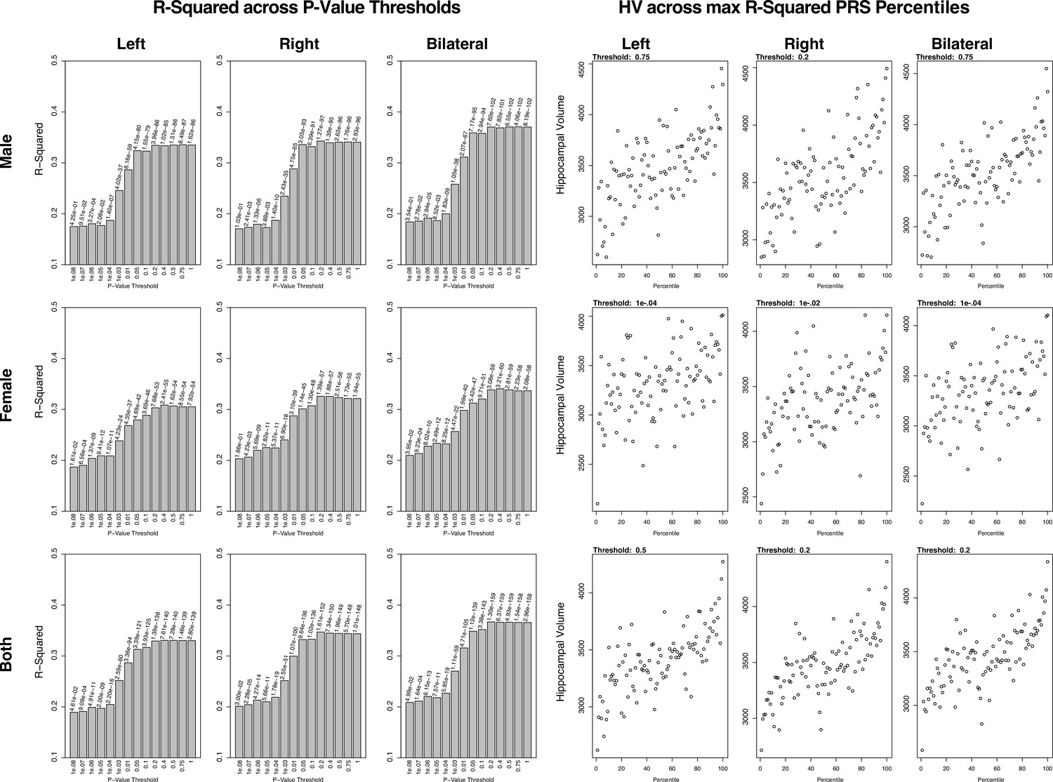
Summary of polygenic scores (PGSs) and models based on hippocampal volume (HV) genome-wide association study (GWAS) and Alzheimer’s Disease Neuroimaging Initiative (ADNI) samples.
The left set of graphs show the R2 of the regression models of polygenic risk score (PRS) across HV for the scores built across SNP p-value thresholds. In contrast to the graphs seen in the UK Biobank (UKB) samples, the R2 values for the most part increase with p-value threshold. The set of graphs on the right show the spread of HV across PGS percentiles, each at the score that had the highest R2 value from the corresponding left graph.
Figure 4 with 3 supplements
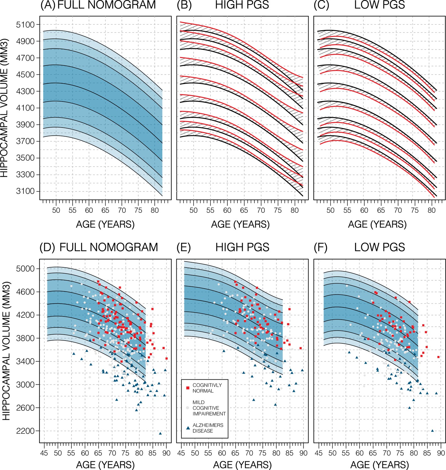
Genetically adjusted nomograms.
Results of genetic adjustment in bilateral male hippocampal volume (HV). (A, D) Nomograms of bilateral HV generated from all male UK Biobank (UKB) samples overlayed with male Alzheimer’s Disease Neuroimaging Initiative (ADNI) samples. Cognitively normal (CN) samples (red squares) centre around the 50th percentile, Alzheimer’s disease (AD) samples (turquoise triangles) lie mostly below the 2.5th percentile, and mild cognitive impairment (MCI) samples (grey circles) span both regions. (B, E) Nomograms generated using only high polygenic score (PGS) samples (top 30%) was shifted upwards (red lines) compared to the original (black lines) by an average of 50 mm3 (1.2% of mean HV). Plotting the high PGS ADNI samples (top 50%) slightly improves intra-group variance. (C, F) Similar results are seen in low PGS samples. Note, the black lines in panels (B, C) are the same as the nomogram in panel (A) and similarly the red lines in panel (B, C) are same as the nomogram in panels (E, F).
Figure 4—figure supplement 1
Genetically adjusted nomograms.
For all sub-figures, the black lines – from top to bottom – represent the 2.5%, 5%, 10%, 25%, 50%, 75%, 90%, 95%, and 97.5% quantiles respectively.
Figure 4—figure supplement 2
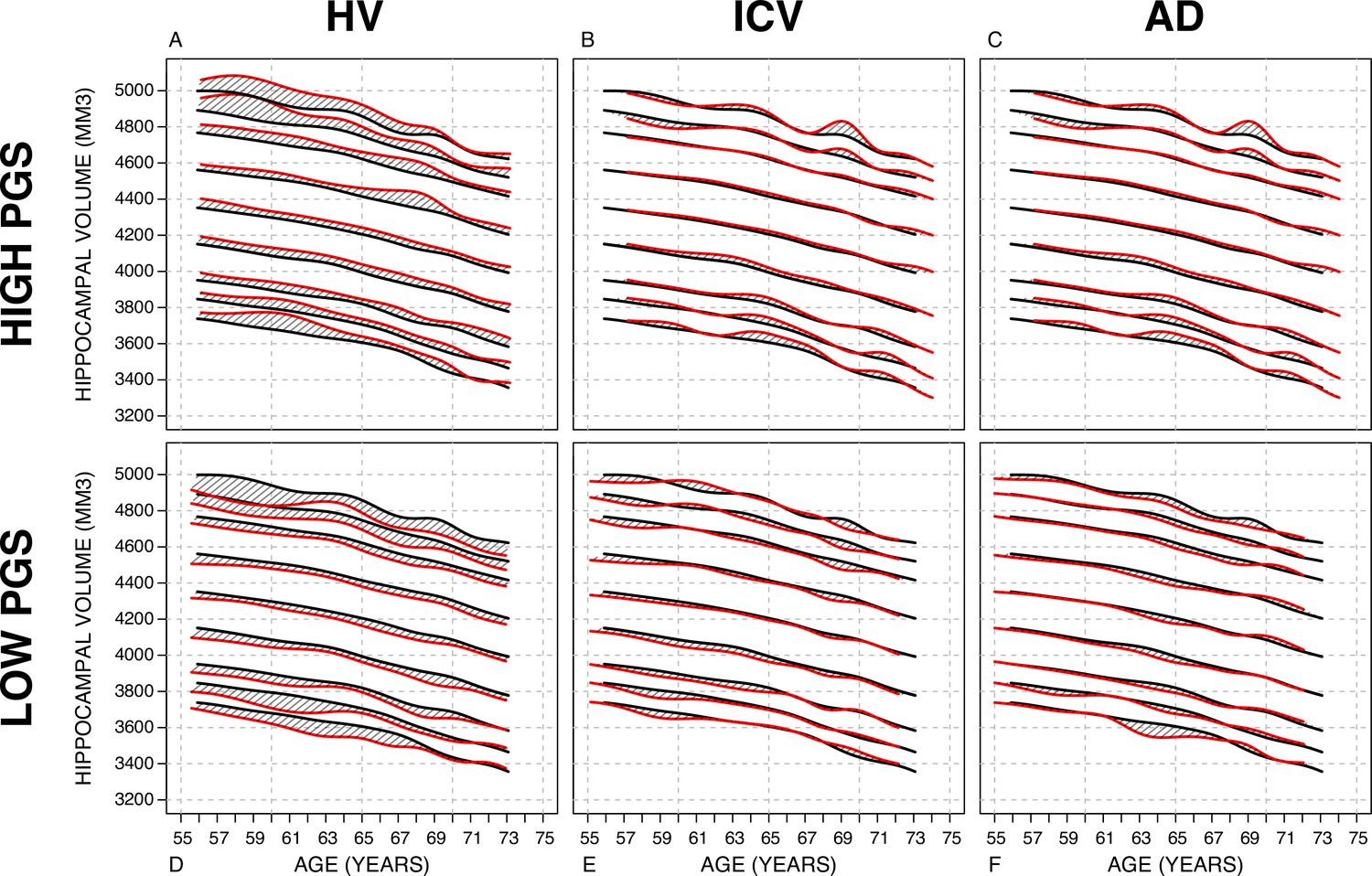
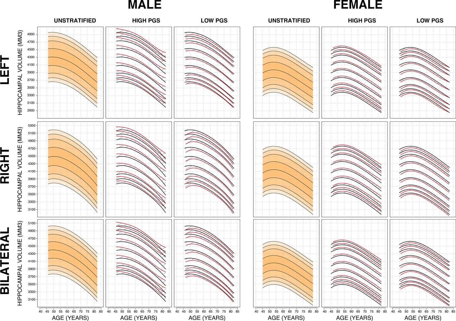
Nomograms generated with the sliding window method (SWM) by stratifying the sample set based on polygenic scores (PGSs).
Left column: PGS based on hippocampal volume (HV) genome-wide association study (GWAS). Middle column: PGS based on intracranial volume (ICV) GWAS. Right column: PGS based on Alzheimer’s disease (AD) GWAS. For all sub-figures, the black lines – from top to bottom – represent the 2.5%, 5%, 10%, 25%, 50%, 75%, 90%, 95%, and 97.5% quantiles, respectively.
Figure 4—figure supplement 3
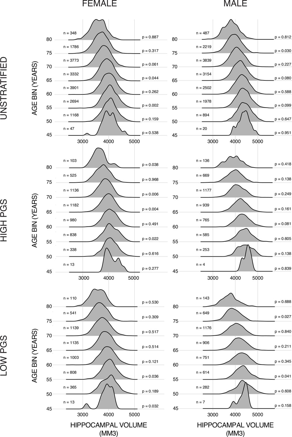
Training data ridge plots.
Histograms of bilateral hippocampal volume (HV) across the different subsets of the datasets. Samples are grouped in bins of 5 years. N is the number of samples in each set and p is the p-value from a Shapiro-Wilks test of normality. Typically, this test would indicate a non-Gaussian distribution with a p-value lower than 0.05 (0.001 corrected for 48 multiple tests in this case).
Figure 5
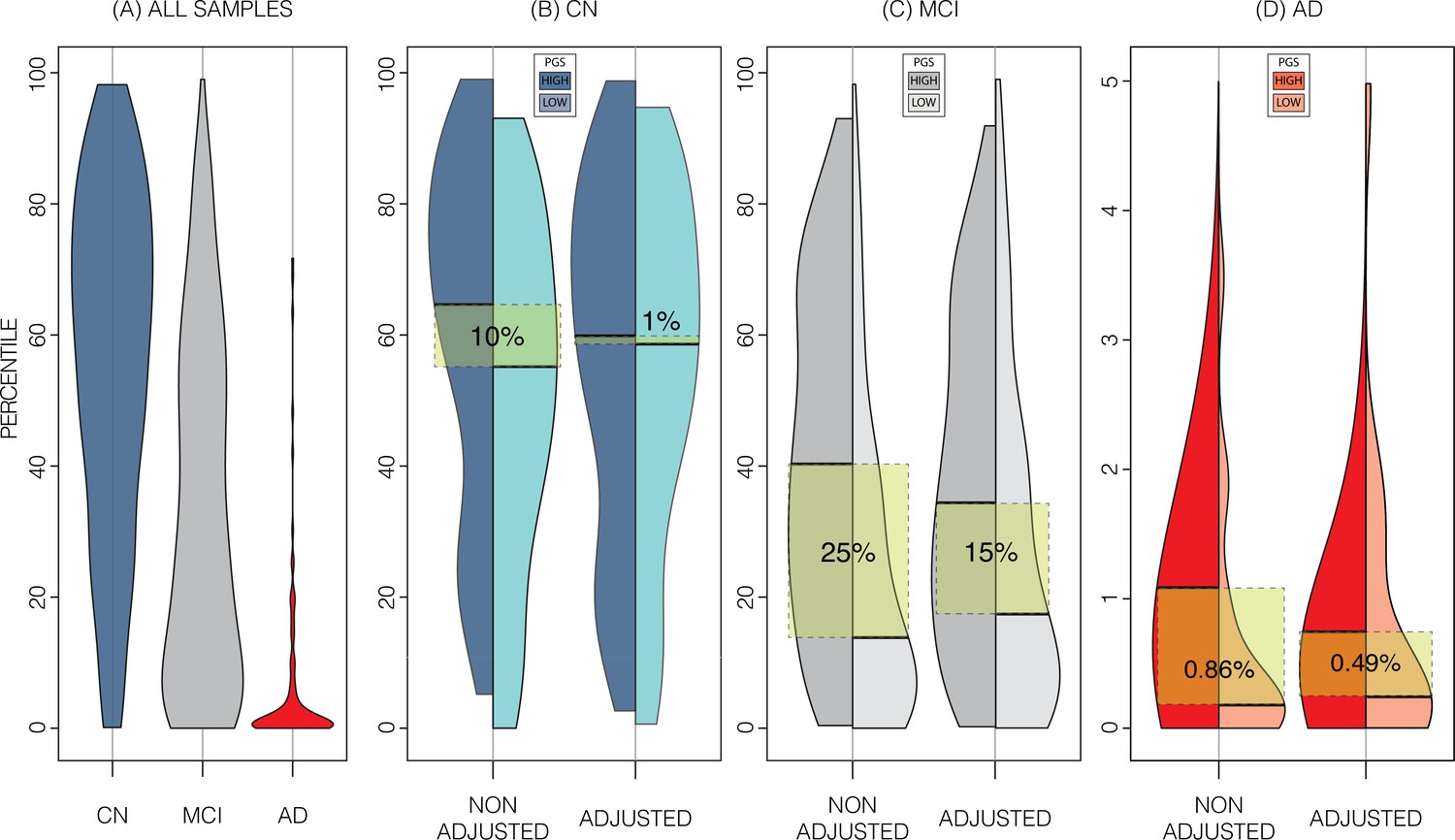
Alzheimer’s Disease Neuroimaging Initiative (ADNI) dataset percentiles in genetically adjusted/non-adjusted nomograms.
Plotting the percentile distribution of the different diagnostic groups across adjusted and non-adjusted nomograms reveals that genetic adjustment increases group cohesiveness. (A) The percentile distributions of the different diagnostic groups against the non-adjusted nomograms. (B) In cognitively normal (CN) samples for example, when plotting against the non-adjusted nomogram (left adjoined boxplots), the median percentile of the top 30% of samples (darker turquoise) was 65%, while the median for the lower 30% of samples (lighter turquoise) was 54%. When using the genetically adjusted nomogram instead (right adjoined boxplots), those median percentiles become 60% and 59% respectively, a 90% relative reduction. Similar results can be seen with mild cognitive impairment (MCI) (C) and Alzheimer’s disease (AD) (D) samples, with 60% and 56% relative reduction, respectively.
-
Figure 5—source data 1
Summary of average percentiles across ADNI strata and UKB nomograms.
- https://cdn.elifesciences.org/articles/78232/elife-78232-fig5-data1-v2.xlsx
Figure 6
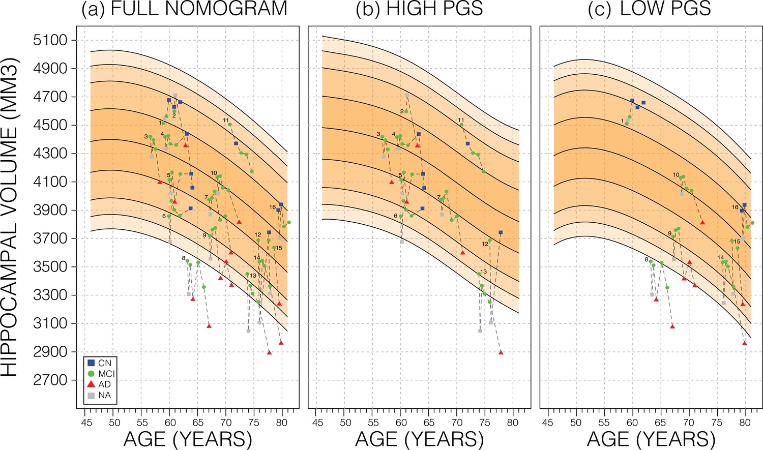
Longitudinal analysis.
A selection of mild cognitive impairment (MCI) samples longitudinal data plotted against nomograms of male mean hippocampal volume (HV). (a) All selected samples plotted against a non-adjusted nomogram. Lines connect visits of the same sample with diagnosis at each visit shown: cognitively normal (CN) as blue squares; MCI as green dots, Alzheimer’s disease (AD) as red triangles, and no diagnosis (NA) as grey squares. (b) Samples from (a) with high polygenic scores (PGS) plotted against a nomogram generated from high PGS CN samples in UK Biobank (UKB). (c) Equivalent result for low PGS samples from (a). For all sub-figures, the black lines – from top to bottom – represent the 2.5%, 5%, 10%, 25%, 50%, 75%, 90%, 95%, and 97.5% quantiles, respectively.
Tables
Table 1
Association between polygenic scores (PGSs) and hippocampal volume (HV).
Linear models were built for HV (left; right; bilateral) using PGS across cohorts (male; female; both) at three representative p-value thresholds (1E-7; 0.01; 1). p-Values of the slope were significant across all categories, with the lowest being associated with the threshold value of 1 in all but a single case (both/right). Variance explained (R2) increased from left to right to bilateral volumes and increased from female to male to both.
| Gender | PGS threshold | LEFT | RIGHT | BILATERAL | ||||||
|---|---|---|---|---|---|---|---|---|---|---|
| Slope(×10–2) | p-Value | R2 | Slope(×10–2) | p-Value | R2 | Slope(×10–2) | p-Value | R2 | ||
| FEMALE | 1E-7 | 10 | 1.8E-46 | 13% | 9.4 | 2.4E-45 | 14% | 11 | 1.4E-51 | 15% |
| 0.01 | 8.2 | 2.7E-26 | 13% | 7.6 | 1.0E-27 | 13% | 8.7 | 3.2E-30 | 14% | |
| 1 | 11 | 9.4E-54 | 13% | 9.62 | 1.5E-48 | 14% | 11 | 1.6E-57 | 15% | |
| MALE | 1E-7 | 8.2 | 1.4E-35 | 18% | 7.5 | 2.6E-35 | 18% | 9.2 | 4.1E-40 | 20% |
| 0.01 | 7.8 | 3.8E-29 | 18% | 6.8 | 3.8E-27 | 18% | 8.6 | 7.8E-32 | 20% | |
| 1 | 9.4 | 3.2E-48 | 18% | 8.0 | 4.7E-43 | 18% | 10 | 9.1E-52 | 20% | |
| BOTH | 1E-7 | 8.4 | 8.1E-90 | 25% | 7.9 | 6.4E-93 | 26% | 9.3 | 3.1E-103 | 28% |
| 0.01 | 7.4 | 9.3E-54 | 24% | 6.7 | 3.3E-53 | 26% | 8 | 2.3E-60 | 28% | |
| 1 | 9.6 | 2.1E-99 | 25% | 8.3 | 1.8E-89 | 26% | 10 | 7.5E-107 | 28% | |
-
Slope = beta coefficient for PGS in the linear mode; p-value for the slope; R2=variance explained by the linear model.
Table 2
Results of ANOVA tests of UK Biobank (UKB) hippocampal volume (HV) percentiles produced with genetically adjusted and unadjusted nomograms.
| SEX | STRATA | DF | SUM SQ | F-VALUE | p-VALUE |
|---|---|---|---|---|---|
| MEN | HIGH | 1 | 18,786 | 22.84 | 1.8E-06 |
| LOW | 1 | 16,407 | 19.96 | 8.04E-06 | |
| WOMEN | HIGH | 1 | 27,068 | 32.92 | 9.97E-09 |
| LOW | 1 | 30,103 | 36.94 | 1.28E-09 |
Additional files
Download links
A two-part list of links to download the article, or parts of the article, in various formats.
Downloads (link to download the article as PDF)
Open citations (links to open the citations from this article in various online reference manager services)
Cite this article (links to download the citations from this article in formats compatible with various reference manager tools)
Nomograms of human hippocampal volume shifted by polygenic scores
eLife 11:e78232.
https://doi.org/10.7554/eLife.78232


