A connectomics-based taxonomy of mammals
Figures
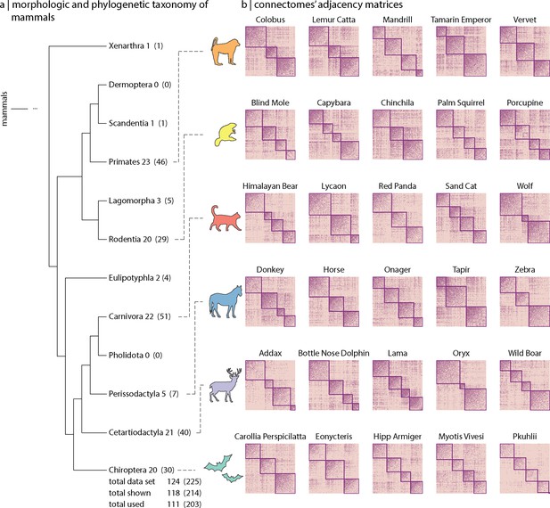
Mammalian MRI (MaMI) data set.
The MaMI data set encompasses high-resolution ex vivo structural and diffusion MRI scans of 124 animal species spanning 12 morphologically and phylogenetically defined taxonomic orders: Cetartiodactyla, Carnivora, Chiroptera, Eulipotyphla, Hyracoidea, Lagomorpha, Marsupialia, Perissodactyla, Primates, Rodentia, Scandentia, and Xenarthra. (a) Hierarchical relationships across 10 (out of the 12 included in the data set) morphological and phylogenetic taxonomic orders. Numbers outside the parenthesis correspond to the number of unique species within each order, and numbers inside the parenthesis correspond to the number of samples (including replicas). (b) Connectivity matrices for five randomly chosen sample species within each of the six orders included in the analyses (i.e. Cetartiodactyla, Carnivora, Chiroptera, Perissodactyla, Primates, and Rodentia). Only orders with at least five different species were included for the analyses. Nodes are organized according to their community affiliation obtained from consensus clustering applied on the connectivity matrix (see ‘Materials and methods’). Communities in (b) correspond to the partition for which the resolution parameter (Figure 1—figure supplement 1).

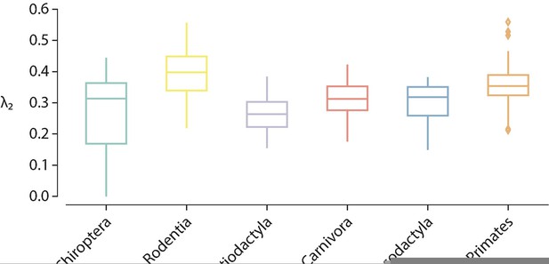
Modularity.
(a) Modularity as a function of resolution the resolution parameter , which controls for the size of the identified modules (see ‘Multi-resolution community detection’). (b) Modularity distributions for each taxonomic order ().
-
Figure 1—figure supplement 1—source data 1
List of animal species.
- https://cdn.elifesciences.org/articles/78635/elife-78635-fig1-figsupp1-data1-v2.zip
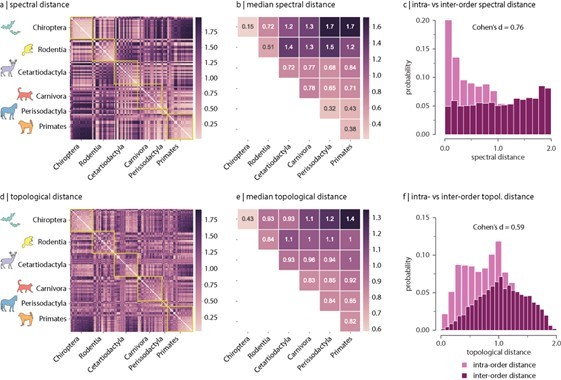
Spectral and topological distance between orders.
(a) Spectral distance between species-specific connectomes. Lower distances indicate greater similarity. Yellow outlines indicate morphologically and genetically defined orders. (b) Median spectral distance within and between all constituent members of each order. (c) Distribution of intra- and inter-order spectral distances. (d) Topological distance between species-specific connectomes. Lower distances indicate greater similarity. Yellow outlines indicate morphologically and genetically defined orders. (e) Median topological distance within and between all constituent members of each order. (f) Distribution of intra- and inter-order topological distances. Effect sizes in (c) and (f) are Cohen’s estimator corresponding to a two-sample Welch’s t-test (). Equivalent conclusions are drawn if common-language effect sizes from the two-sample Mann–Whitney U-test are used.

Laplacian eigenspectra.
Spectral plots were obtained by convolving the eigenspectrum of the normalized Laplacian matrix of the graph with a Gaussian kernel. The eigenvalues of the normalized Laplacian of the connectivity matrix, and their multiplicities, capture distinct topological properties of the graph (Banerjee and Jost, 2009; Banerjee and Jost, 2008; Newman, 2001; Grone et al., 1990; Grone and Merris, 1994; Das, 2004), thus acting like a spectroscopy of its underlying topology. More importantly, it has the advantage of situating graphs of different sizes and with non-homologous node correspondence in a common frame of reference in which they can be compared.
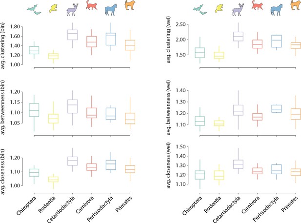
Distribution of local graph features across taxonomic orders.
Distributions of average local features are shown for each order. Features are normalized relative to a set of 1000 randomly rewired graphs that preserve the degree sequence and distribution of the nodes (Maslov and Sneppen, 2002). Features are computed for both the binary (left) and weighted (right) connectomes.
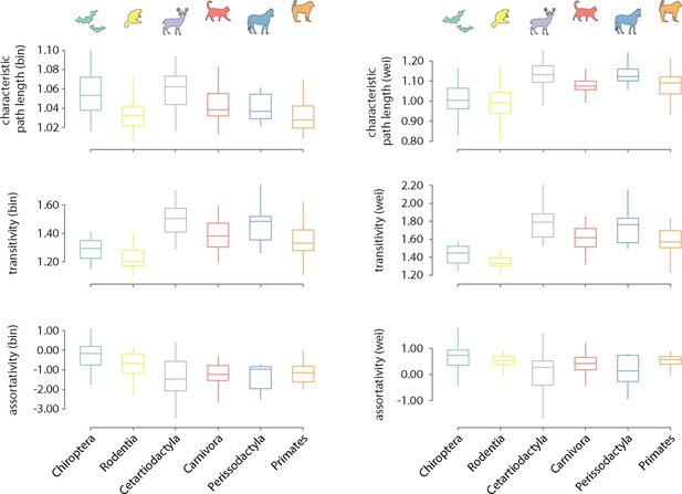
Distribution of global graph features across taxonomic orders.
Distributions of global features are shown for each order. Features are normalized relative to a set of 1000 randomly rewired graphs that preserve the degree sequence and distribution of the nodes (Maslov and Sneppen, 2002). Features are computed for both the binary (left) and weighted (right) connectomes.

Cumulative distribution of binary local graph features across taxonomic orders.
The cumulative distributions of individual features are shown for each individual sample within each order.

Cumulative distribution of weighted local graph features across taxonomic orders.
The cumulative distributions of individual features are shown for each individual sample within each order.
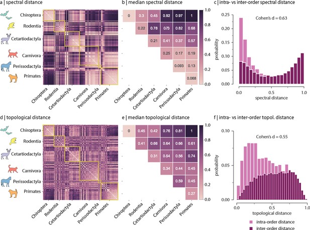
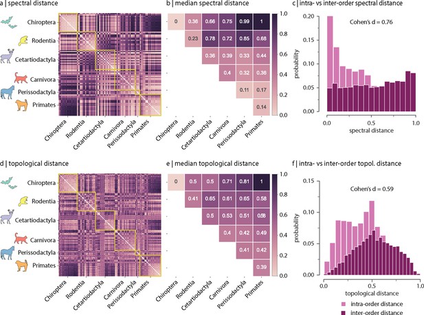
Effect of using replicated samples on the topological and spectral distance between orders.
All samples, including replicas, were used to estimate inter-species spectral and topological distance. (a) Spectral distance between species-specific connectomes. (b) Median spectral distance within and between all constituent members of each order. (c) Distribution of intra- and inter-order spectral distances. (d) Topological distance between species-specific connectomes. (e) Median topological distance within and between all constituent members of each order. (f) Distribution of intra- and inter-order topological distances. Effect sizes in (c) and (f) are Cohen’s estimator corresponding to a two-sample Welch’s t-test (). Equivalent conclusions are drawn if common-language effect sizes from the two-sample Mann-Whitney U-test are used.

Effect of (decreasing) parcellation resolution on the spectral and topological inter-species distance.
Results were replicated using a 100-node parcellation. (a) Spectral distance between species-specific connectomes. (b) Median spectral distance within and between all constituent members of each order. (c) Distribution of intra- and inter-order spectral distances. (d) Topological distance between species-specific connectomes. (e) Median topological distance within and between all constituent members of each order. (f) Distribution of intra- and inter-order topological distances. Effect sizes in (c) and (f) are Cohen’s estimator corresponding to a two-sample Welch’s t-test (). Equivalent conclusions are drawn if common-language effect sizes from the two-sample Mann-Whitney U-test are used.

Effect of (increasing) parcellation resolution on the spectral and topological inter-species distance.
Results were replicated using a 300-node parcellation. (a) Spectral distance between species-specific connectomes. (b) Median spectral distance within and between all constituent members of each order. (c) Distribution of intra- and inter-order spectral distances. (d) Topological distance between species-specific connectomes. (e) Median topological distance within and between all constituent members of each order. (f) Distribution of intra- and inter-order topological distances. Effect sizes in (c) and (f) are Cohen’s estimator corresponding to a two-sample Welch’s t-test (). Equivalent conclusions are drawn if common-language effect sizes from the two-sample Mann–Whitney U-test are used.
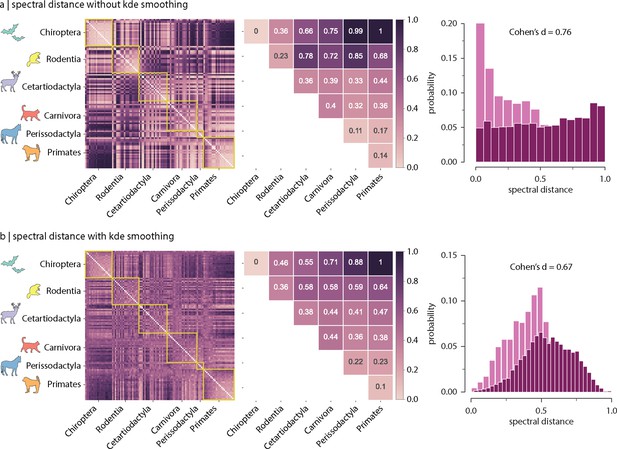
Effect of kernel density estimation (kde) on inter-species spectral distances.
To allow comparison with previous reports, Gaussian kde smoothing is applied to the Laplacian eigenspectrum of individual species, before estimating inter-species distances. Spectral distance with (a) and without (b) kernel density estimation smoothing. Left: inter-species spectral distance. Centre: median inter-species spectral distance. Right: intra- vs. inter-order spectral distance distributions. Effect sizes correspond to Cohen’s estimator from a two-sample Welch’s t-test ().
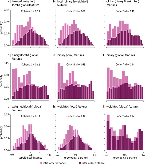
Contribution of network features.
Topological distance can be computed using different combinations of local and global, binary and weighted connectome features. Histograms show intra- and inter-order distance distributions when using (a) all (binary, weighted, local, and global), (b) all local (binary and weighted), (c) all global (binary and weighted), (d) all binary (local and global), (e) only binary local, (f) only binary global, (g) all weighted (local and global), (h) only weighted local, and (i) only weighted global features. Local features include (the average and standard deviation of) degree, clustering, betweenness, and closeness. Global features include characteristic path length, transitivity, and assortativity. For definitions, please see ‘Materials and methods.’ Effect sizes correspond to Cohen’s estimator from a two-sample Welch’s t-test. Equivalent conclusions are drawn if common-language effect sizes from a two-sample Mann–Whitney U-test are used. In all cases, the difference in the mean and median of intra- and inter-order distance distributions is statistically significant (). The same conclusions can be drawn after controlling for network density (Figure 3—figure supplement 6).
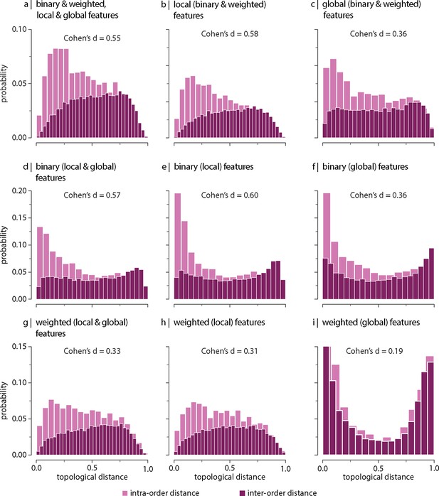
Effect of using replicated samples on the contribution of network features.
All samples, including replicas, were used to estimate inter-species topological distance. Topological distance can be computed using different combinations of local and global, binary and weighted connectome features. Histograms show intra- and inter-order distance distributions when using (a) all (binary, weighted, local, and global), (b) all local (binary and weighted), (c) all global (binary and weighted), (d) all binary (local and global), (e) only binary local, (f) only binary global, (g) all weighted (local and global), (h) only weighted local, and (i) only weighted global features. Local features include (the average and standard deviation of) degree, clustering, betweenness, and closeness. Global features include characteristic path length, transitivity, and assortativity. Effect sizes correspond to Cohen’s estimator from a two-sample Welch’s t-test. Equivalent conclusions are drawn if common-language effect sizes from a two-sample Mann–Whitney U-test are used. In all cases, the difference in the mean and median of intra- and inter-order distance distributions is statistically significant ().
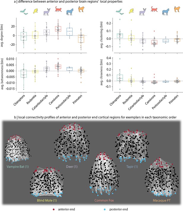
Changes in local topology along the anterior–posterior axis.
(a) Distribution across taxonomic orders of the difference in average local network topology between the 10% most anterior and the 10% most posterior brain regions (i.e. the anterior–posterior difference). Local features considered include: binary (average) degree, clustering, betweenness centrality and closeness. (b) Top 5% strongest connections of the 10% most anterior (red) and the 10% most posterior (blue) brain regions for exemplar species within each taxonomic order. Separate one-way ANOVAs were performed to compare the effect of taxonomic order on anterior–posterior differences in local: (i) degree: , , (ii) clustering: , , (iii) betweenness: , ; and (iv) closeness: , .
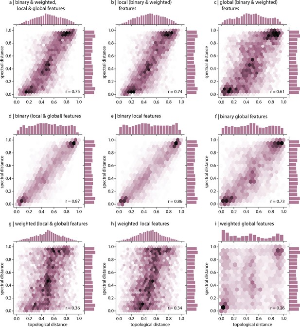
Relationship between spectral and topological distance.
Pearson’s correlation between inter-species distances computed using topological distance (abscissa) and spectral distance (ordinate). Correlations are shown for (a) all (binary, weighted, local, and global), (b) all local (binary and weighted), (c) all global (binary and weighted), (d) all binary (local and global), (e) only binary local, (f) only binary global, (g) all weighted (local and global), (h) only weighted local, and (i) only weighted global features.
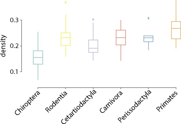
Network density.
Distribution of network density is shown for each taxonomic order. Connection density is estimated as the ration of existent connections to the total number of possible connections.

Controlling for network density.
Network density is regressed out from (a) binary local, (b) weighted local, (c) binary global and (d) weighted global topological features (see ‘Materials and methods’).
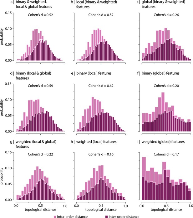
Contribution of network features after controlling for network density.
Network density is regressed out from topological features (see ‘Materials and methods’), and topological distance is computed using multiple local and global connectome features. Histograms show intra- and inter-order distance distributions when using (a) all (binary, weighted, local, and global), (b) all local (binary and weighted), (c) all global (binary and weighted), (d) all binary (local and global), (e) only binary local, (f) only binary global, (g) all weighted (local and global), (h) only weighted local, and (i) only weighted global features. Local features include (the average and standard deviation of) degree, clustering, betweenness, and closeness. Global features include characteristic path length, transitivity, and assortativity. For definitions please see ‘Materials and methods.’ Effect sizes correspond to Cohen’s estimator from a two-sample Welch’s t-test. Equivalent conclusions are drawn if common-language effect sizes from a two-sample Mann–Whitney U-test are used. In all cases, the difference in the mean and median of intra- and inter-order distance distributions is statistically significant ().

Taxonomic order separation in low-dimensional space.
Multidimensional scaling (MDS) with cosine distance is applied to (a) spectral and (b–j) topological features to generate a low-dimensional (2D) projection of the data set. MDS was implemented using the MDS function in the manifold module of the Scikit-learn Python package (Pedregosa et al., 2011). Details of the implementation can be found in the publicly available code repository. Specifically, MDS was applied to (a) the Laplacian eigenspectra, (b) all (binary, weighted, local, and global), (c) all local (binary and weighted), (d) all global (binary and weighted), (e) all binary (local and global), (f) only binary local, (g) only binary global, (h) all weighted (local and global), (i) only weighted local, and (j) only weighted global features. Local features include (the average and standard deviation of) degree, clustering, betweenness, and closeness. Global features include characteristic path length, transitivity, and assortativity. Each dot in the scatter plots represents a sample from a different order. Visual inspection of the 2D projections shows that, generally speaking, local features tend to provide a better class separation compared to global features.
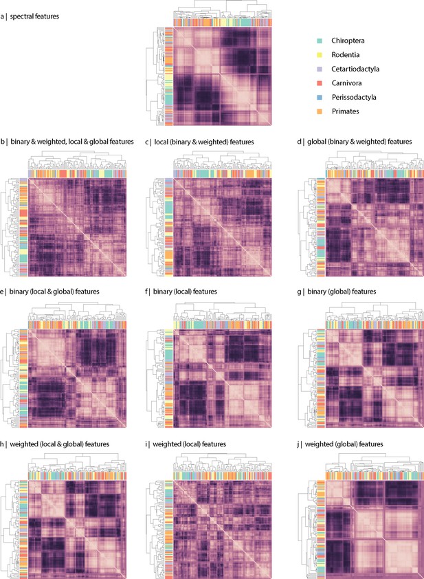
Connectome-based clustering of mammals.
Hierarchical clustering was applied to the (a) spectral and (b–j) topological distance matrices to assess the extent to which data-driven clustering of mammalian species recapitulates traditional taxonomies based on morphology and genetics. Hierarchical clustering was implemented using the hierarchy.linkage function in the cluster module of the Scipy Python package (Virtanen et al., 2020). Details of the implementation can be found in the publicly available code repository. Specifically, hierarchical clustering was applied to the inter-species distance matrix estimated using (a) the Laplacian eigenspectra, (b) all (binary, weighted, local, and global), (c) all local (binary and weighted), (d) all global (binary and weighted), (e) all binary (local and global), (f) only binary local, (g) only binary global, (h) all weighted (local and global), (i) only weighted local, and (j) only weighted global topological features. Local features include (the average and standard deviation of) degree, clustering, betweenness, and closeness. Global features include characteristic path length, transitivity, and assortativity. Each heat map represents an inter-species distance matrix. Coloured rectangles represent the order each sample belongs to. Visual inspection of the results shows that, generally speaking, local features tend to provide a clustering solution that resembles more traditional taxonomies.
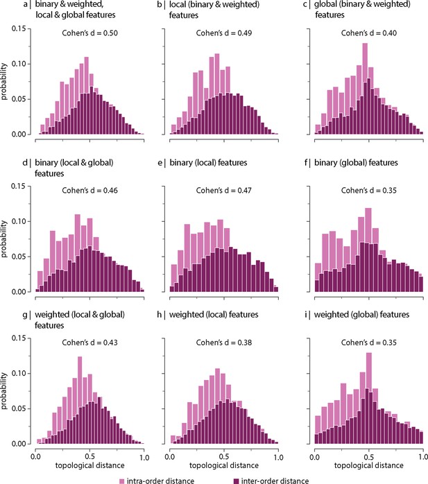
Effect of (decreasing) parcellation resolution on the contribution of topological network features.
Results were replicated using a 100-node parcellation. Topological distance can be computed using different combinations of local and global, binary and weighted connectome features. Histograms show intra- and inter-order distance distributions when using (a) all (binary, weighted, local, and global), (b) all local (binary and weighted), (c) all global (binary and weighted), (d) all binary (local and global), (e) only binary local, (f) only binary global, (g) all weighted (local and global), (h) only weighted local, and (i) only weighted global features. Local features include (the average and standard deviation of) degree, clustering, betweenness, and closeness. Global features include characteristic path length, transitivity, and assortativity. For definitions, please see ‘Materials and methods.’ Effect sizes correspond to Cohen’s estimator from a two-sample Welch’s t-test. Equivalent conclusions are drawn if common-language effect sizes from a two-sample Mann–Whitney U-test are used. In all cases, the difference in the mean and median of intra- and inter-order distance distributions is statistically significant ().

Effect of (increasing) parcellation resolution on the contribution of topological network features.
Results were replicated using a 300-node parcellation. Topological distance can be computed using different combinations of local and global, binary and weighted connectome features. Histograms show intra- and inter-order distance distributions when using (a) all (binary, weighted, local, and global), (b) all local (binary and weighted), (c) all global (binary and weighted), (d) all binary (local and global), (e) only binary local, (f) only binary global, (g) all weighted (local and global), (h) only weighted local, and (i) only weighted global features. Local features include (the average and standard deviation of) degree, clustering, betweenness, and closeness. Global features include characteristic path length, transitivity, and assortativity. For definitions, please see ‘Materials and methods.’ Effect sizes correspond to Cohen’s estimator from a two-sample Welch’s t-test. Equivalent conclusions are drawn if common-language effect sizes from a two-sample Mann–Whitney U-test are used. In all cases, the difference in the mean and median of intra- and inter-order distance distributions is statistically significant ().
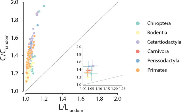
Conservation of small-world architecture.
Clustering coefficient vs. characteristic path length normalized relative to a set of 1000 randomly rewired graphs that preserve the degree sequence of the nodes (Maslov and Sneppen, 2002). For definitions of each graph measure, see ‘Materials and methods.’ Each data point represents a different animal species. Data points above the identity line are said to have small-world architecture. The inset on the right bottom corner is a zoom on the abscissa; dots correspond to the median and error bars correspond to the standard deviation across species within the same taxonomic order.
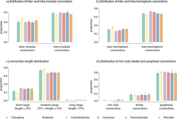
Contribution of edge types.
Mean proportion of (a) inter- and intra-modular connections, (b) inter- and intra-hemispheric connections, (c) short- (length ≤ 25%), medium- (25% < length ≤ 75%) and long-range connections (length ≥ 75%), and (d) rich-club (connecting two rich-club nodes), feeder (connecting one rich-club and one non-rich-club node) and peripheral (connecting two non-rich-club nodes) connections. Error bars indicate 95% confidence intervals.

Connection length distribution.
The connection length distributions of individual species for each taxonomic order.


