Optogenetics and electron tomography for structure-function analysis of cochlear ribbon synapses
- Molecular Architecture of Synapses Group, Institute for Auditory Neuroscience and InnerEarLab, University Medical Center Göttingen, Germany
- Center for Biostructural Imaging of Neurodegeneration, University Medical Center Göttingen, Germany
- Collaborative Research Center 889 "Cellular Mechanisms of Sensory Processing", Germany
- Institute for Auditory Neuroscience and InnerEarLab, University Medical Center Göttingen, Germany
- Auditory Neuroscience & Synaptic Nanophysiology Group, Max Planck Institute for Multidisciplinary Sciences, Germany
- Göttingen Graduate School for Neuroscience and Molecular Biosciences, University of Göttingen, Germany
- Faculty of Agriculture, South Westphalia University of Applied Sciences, Germany
- NanoTag Biotechnologies GmbH, Germany
- Institute of Neuro- and Sensory Physiology, University Medical Center Göttingen, Germany
- Multiscale Bioimaging: from Molecular Machines to Networks of Excitable Cells, Germany
- Synaptic Physiology of Mammalian Vestibular Hair Cells Group, Institute for Auditory Neuroscience and InnerEarLab, University Medical Center Göttingen, Germany
Figures
Figure 1 with 1 supplement
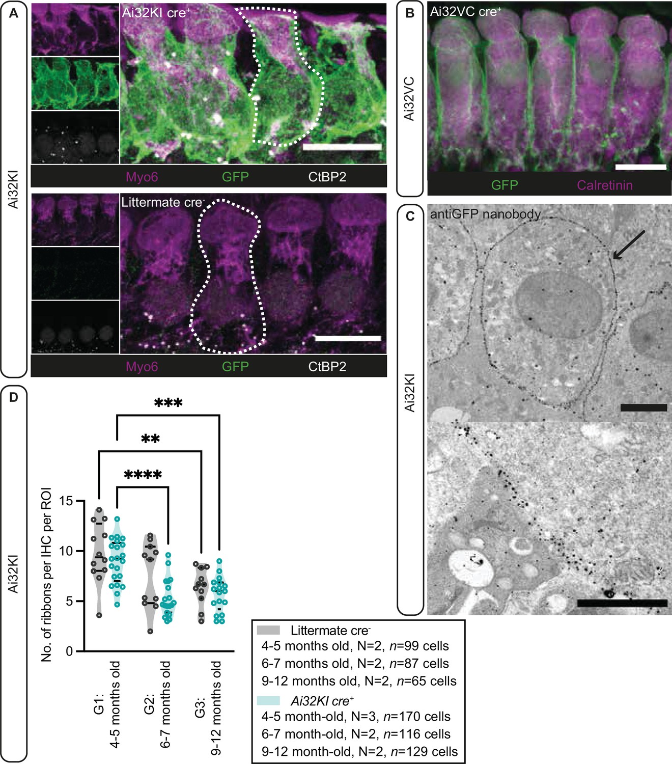
Plasma membrane expression of ChR2 in inner hair cells (IHCs).
(A) IHCs express ChR2 in the plasma membrane. Maximal projection of confocal Z-stacks from the apical turn of the anti-GFP labeled organ of Corti from a 4- to 5-month-old Ai32KI cre+ mice (upper panel) and its littermate control (WT) (lower panel). Myo6 (magenta) was used as counterstaining and CtBP2 labeling shows ribbons at the basolateral pole of IHCs (examples outlined). ChR2 expression (green) is observed along the surface of Ai32KI cre+ IHCs (upper panel) but not in WT IHCs (lower panel). Scale bar, 10 μm. (B) Maximal intensity projection of confocal Z-stacks from the apical coil of anti-GFP labeled Ai32VC cre+ IHCs. Calretinin immunostaining was used to delineate the IHC cytoplasm. Scale bar, 10 µm. (C) Pre-embedding immunogold labeling for electron microscopy was performed with a gold-coupled anti-GFP nanobody recognizing the EYFP of the ChR2 construct. A clear localization at the plasma membrane of IHCs is visible (arrow, upper panel). Scale bar, 2 μm. The magnified image of the membrane labeling is shown in the lower panel. Scale bar, 1 μm. (D) The average number of ribbons per IHC is similar between ChR2-expressing IHCs and WT IHCs. Both Ai32KI cre+ and WT mice showed a comparable decrease in the number of ribbons with age (**p<0.01, ***p<0.001, ****p<0.0001; two-way ANOVA followed by Tukey’s test for multiple comparisons). N=Number of animals. Violin plots show median and quartiles with data points overlaid.
Figure 1—figure supplement 1
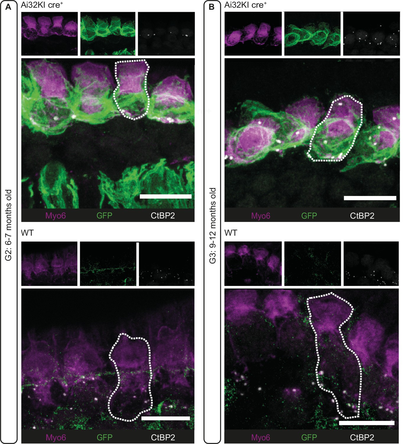
Long-term expression of ChR2 at inner hair cell (IHC) plasma membrane.
Maximal projection of confocal Z-stacks of (A) G2 (6- to 7-month-old mice) and (B) G3 (9- to 12-month-old mice) IHCs from the apical turn of organs of Corti from ChR2-expressing mice (Ai32KI cre+; upper panels) and their respective controls (WT; lower panels). Some IHCs are outlined with a dotted line. ChR2 expression at the membrane is visualized by GPF labeling (green). Myo6 (magenta) immunostaining was used to delineate the IHC and CtBP2 to visualize the ribbons (white). Ectopic GFP expression (A, upper panel) in spiral ganglion fibers is indicative of unspecific cre recombination (see Materials and methods). Scale bars, 10 µm.
Figure 2 with 1 supplement
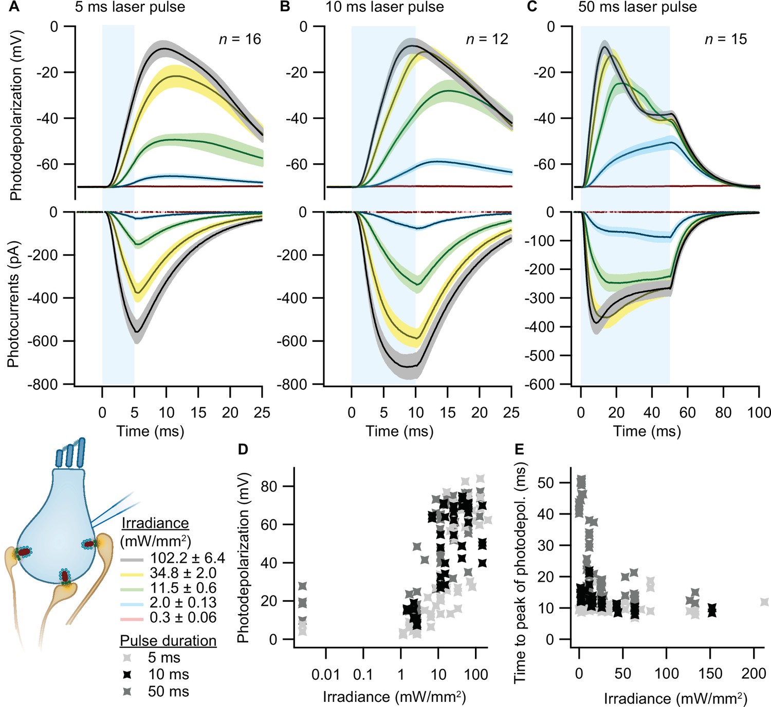
Optogenetic depolarization of inner hair cells (IHCs).
IHCs expressing ChR2 (Ai32VC cre+ and Ai32KI cre+) were optogenetically stimulated by 473 nm light pulses of increasing irradiance (mW/mm2; presented as mean ± SEM). (A–C) Average photocurrents (lower panel) and photodepolarizations (upper panel) of patch-clamped IHCs during 5 ms (A, ncells = 16, Nanimals = 7), 10 ms (B, ncells = 12, Nanimals = 4), and 50 ms (C, ncells = 15; Nanimals = 6) light pulses of increasing irradiances (color coded). Mean is displayed by the continuous line and ± SEM by the shaded area. (D–E) Peak of photodepolarization (D) and time to peak (E) obtained for increasing irradiances of different lengths (light gray 5 ms, black 10 ms, dark gray 50 ms).
Figure 2—figure supplement 1
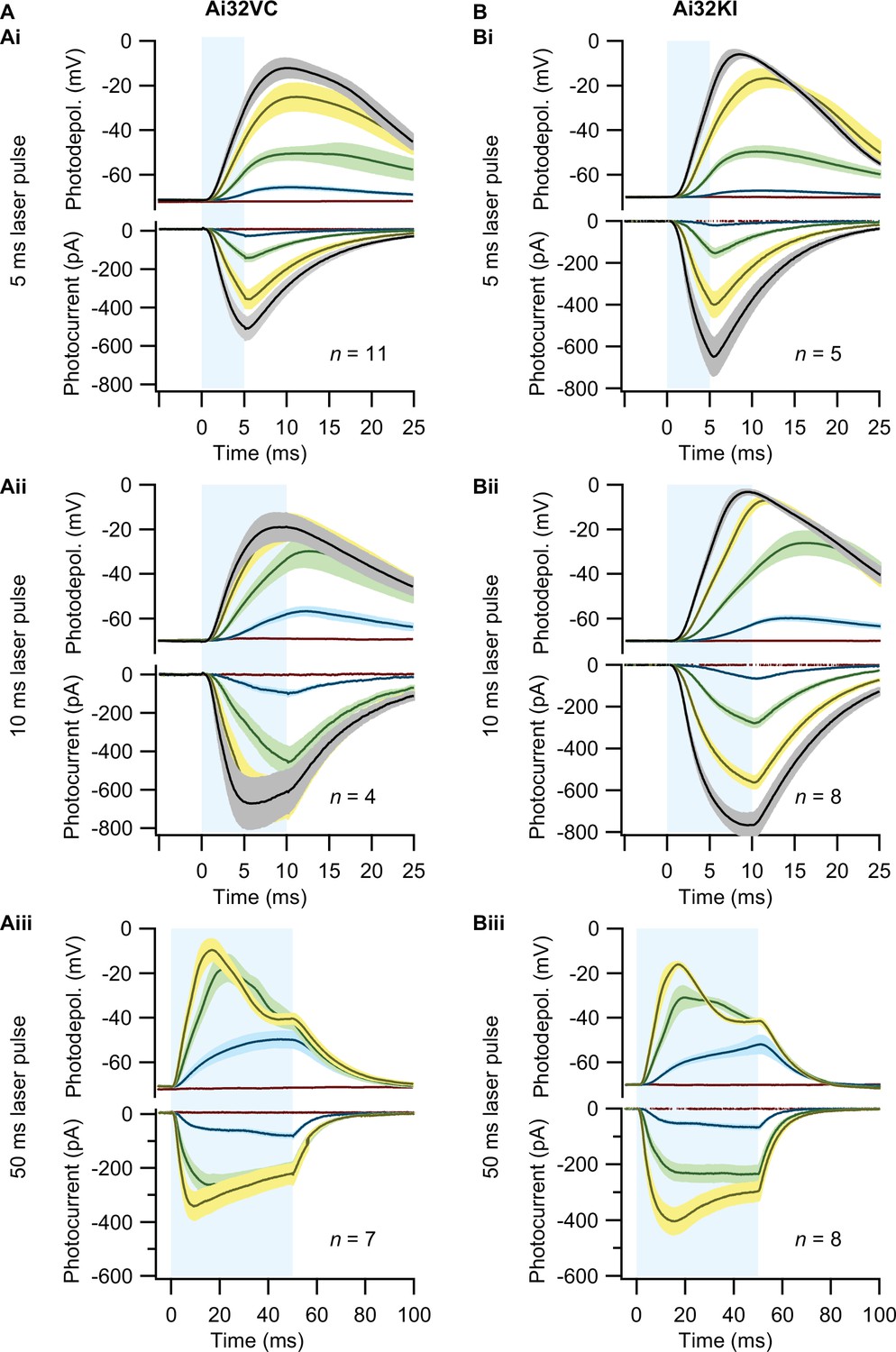
Comparison of optogenetic stimulation of inner hair cells (IHCs) from Ai32VC cre+ and Ai32KI cre+ mice.
IHCs expressing ChR2 (Ai32VC cre+ left and Ai32KI cre+ right) were optogenetically stimulated by 473 nm light pulses of increasing irradiance (mW/mm2). (A–C) Average photocurrents (lower panel) and photodepolarizations (upper panel) of patch-clamped IHCs during 5 ms (A), 10 ms (B), and 50 ms light pulses of increasing irradiances (color coded as in Figure 2). Mean is displayed by the continuous line and ± SEM by the shaded area. For 5 ms: nAi32VC=11, Nanimals Ai32VC=6; nAi32KI=5, Nanimals Ai32KI=1. For 10 ms: nAi32VC=4, Nanimals Ai32VC=1; nAi32KI=8, Nanimals Ai32KI=3. For 50 ms: nAi32VC=7, Nanimals Ai32VC=3; nAi32KI=8, Nanimals Ai32KI=3.
Figure 3 with 1 supplement

Opto-high-pressure freezing machine (HPM) setup and irradiance calculation for the HPM.
(A) Simplified illustration depicting the components of the external setup installed to control the light stimulation (irradiance and duration), to determine the time point of the freezing onset and command relay (blue, control unit) to the sensors (accelerometer [red, outside, AM], microphone [patterned blue, inside, M], pneumatic pressure sensor, green, inside, PS) to initiate the mechanical sensing process of the HPM100 (Source code 3). (B) Fiber – cartridge arrangement in the HPM100 with the fiber at an angle of 60° to the upper half-cylinder: Sample plane: black, fiber: gray, Light rays: red. Mechanical components of HPM100 are not shown. (C) Sample loading scheme. (D) Re-build chamber replica to enable irradiance calculation externally. (E) CCD image of the photodiode in the sample plane. (F) The spatial irradiance distribution with a peak irradiance of ~6 mW/mm2 at 80% intensity of the light-emitting diode (LED) was calculated using a self-written MATLAB routine intensityprofilcalculator.m (Source code 4). Depicted are pixel values in irradiance. The complete workflow for Opto-HPF is presented in Figure 3—figure supplement 1.
Figure 3—figure supplement 1
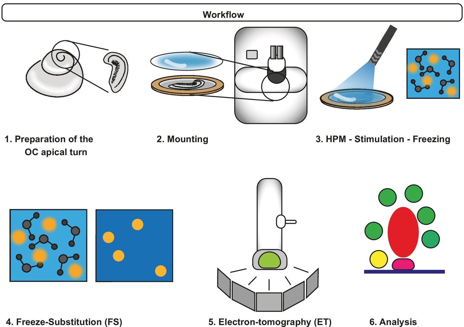
Workflow of Opto-HPF.
After dissection of the organ of Corti (OC), the sample is mounted and inserted in the high-pressure freezing machine (HPM). The blue light stimulation occurs in the HPM freezing chamber with subsequent freezing. Finally, freeze substitution is performed followed by electron tomography (ET) and data analysis.
Figure 4
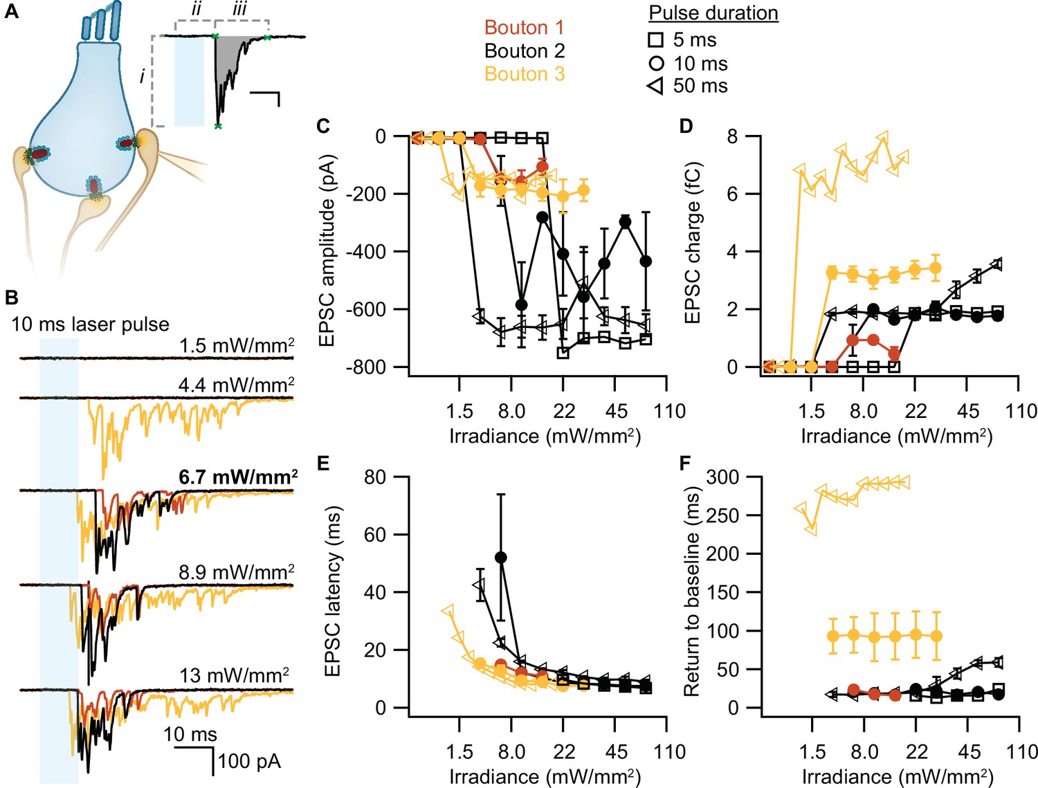
Optogenetically-triggered exocytosis at individual ribbon synapses.
(A) Excitatory postsynaptic currents (EPSCs) upon the optogenetic stimulation of Ai32VC cre+ inner hair cells (IHCs) were recorded using whole-cell patch-clamp of the contacting bouton. The response was quantified in terms of EPSC amplitude (i), charge (gray area), latency (ii), and return to baseline (iii) (Source code 2). Scale bar as in panel B. (B) Recorded EPSCs from three different postsynaptic boutons (different colors for boutons 1–3) in response to increasing light intensities. (C–F) Amplitude (C), charge (D), latency (E), and return to baseline (F) of the light triggered EPSCs to different light pulse durations (5 ms squares; 10 ms circles; 50 ms triangles). nboutons= 3, Nanimals= 2.
Figure 5
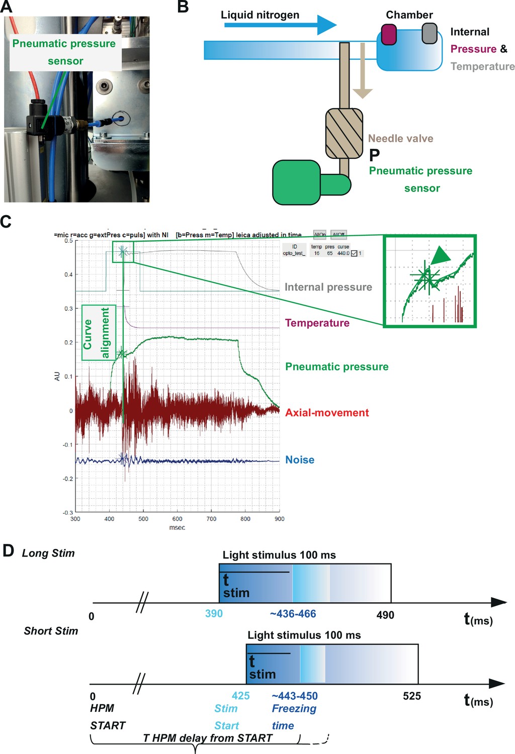
Correlating the sensor signals to internal pressure and temperature measured inside the high-pressure freezing machine (HPM).
(A) Pneumatic pressure sensor inside the HPM100. (B) Scheme of the localization of the pneumatic pressure sensor below the pneumatic needle valve, which allows LN2 influx in the chamber for freezing. (C) Depicted are the curves from the different sensors aligned by using the MATLAB GUI (Source code 5). The curves of the pressure build-up start and temperature corresponding decline are aligned to the steep drop in the pneumatic pressure curve (green arrowhead, inset). (D) The outline of the optical stimulation incorporated with HPF: 100 ms light pulse set to a 390 ms delay from HPM start resulted in a stimulation duration of 48–76 ms before freezing (‘LongStim’) and that set to a 425 ms delay from HPM start in a stimulation of 17–25 ms (‘ShortStim’).
Figure 6 with 2 supplements
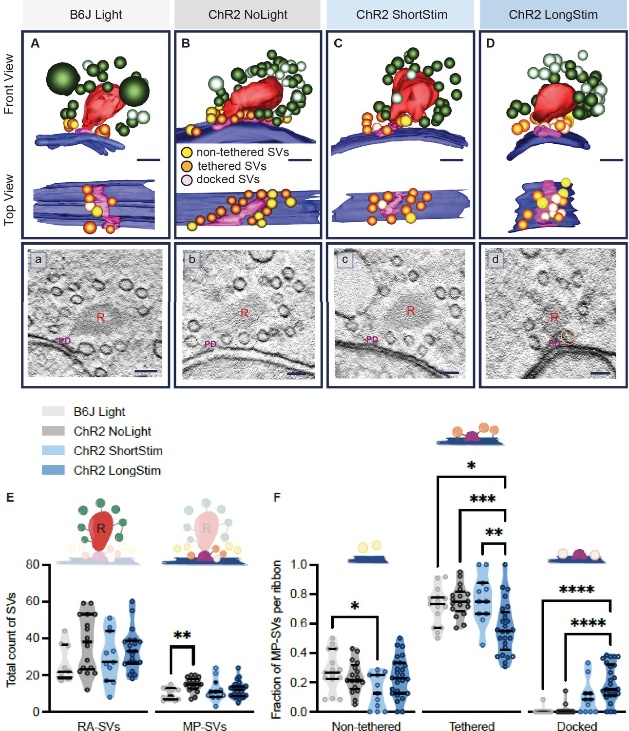
Functional active zone (AZ) states differ in their morphologically defined vesicle pools.
Representative tomographic 3D reconstructions of AZs at (A) B6J Light, (B) ChR2 NoLight, (C) ChR2 ShortStim, and (D) ChR2 LongStim conditions displayed in both front view (upper part of the panel) and top view (ribbon removed from the model, lower part of the panel). (a–d) Corresponding virtual sections of A–B. The AZ membrane is shown in blue, presynaptic density in pink (and indicated with PD), ribbons in red (and indicated with R), membrane-proximal (MP)-synaptic vesicles (SVs) (non-tethered in yellow, tethered in orange and docked in light pink), ribbon-associated (RA)-SVs (green, light green). Magnification ×12,000; scale bars, 100 nm. (E) Total count of SVs per pool (RA- and MP-SV pools), per ribbon. (F) The fraction of non-tethered, tethered, and docked MP-SVs per ribbon. Data are presented in mean ± SEM. *p<0.05, **p<0.01, ***p<0.001, and ****p<0.0001. Statistical test: one-way ANOVA followed by Tukey’s test (parametric data) and Kruskal-Wallis (KW) test followed by Dunn’s test (non-parametric data). MP-SV pool: B6J Light: nribbons = 15, Nanimals = 2. ChR2 NoLight: nribbons = 17, Nanimals = 4. ChR2 ShortStim: nribbons = 11, Nanimals = 1. ChR2 LongStim: nribbons = 26, Nanimals = 4. RA-SV pool: B6J Light: nribbons = 9, Nanimals = 1, ChR2 NoLight: nribbons = 17, Nanimals = 4. ChR2 ShortStim: nribbons = 11, Nanimals = 1. ChR2 LongStim: nribbons = 21, Nanimals = 3.
Figure 6—figure supplement 1
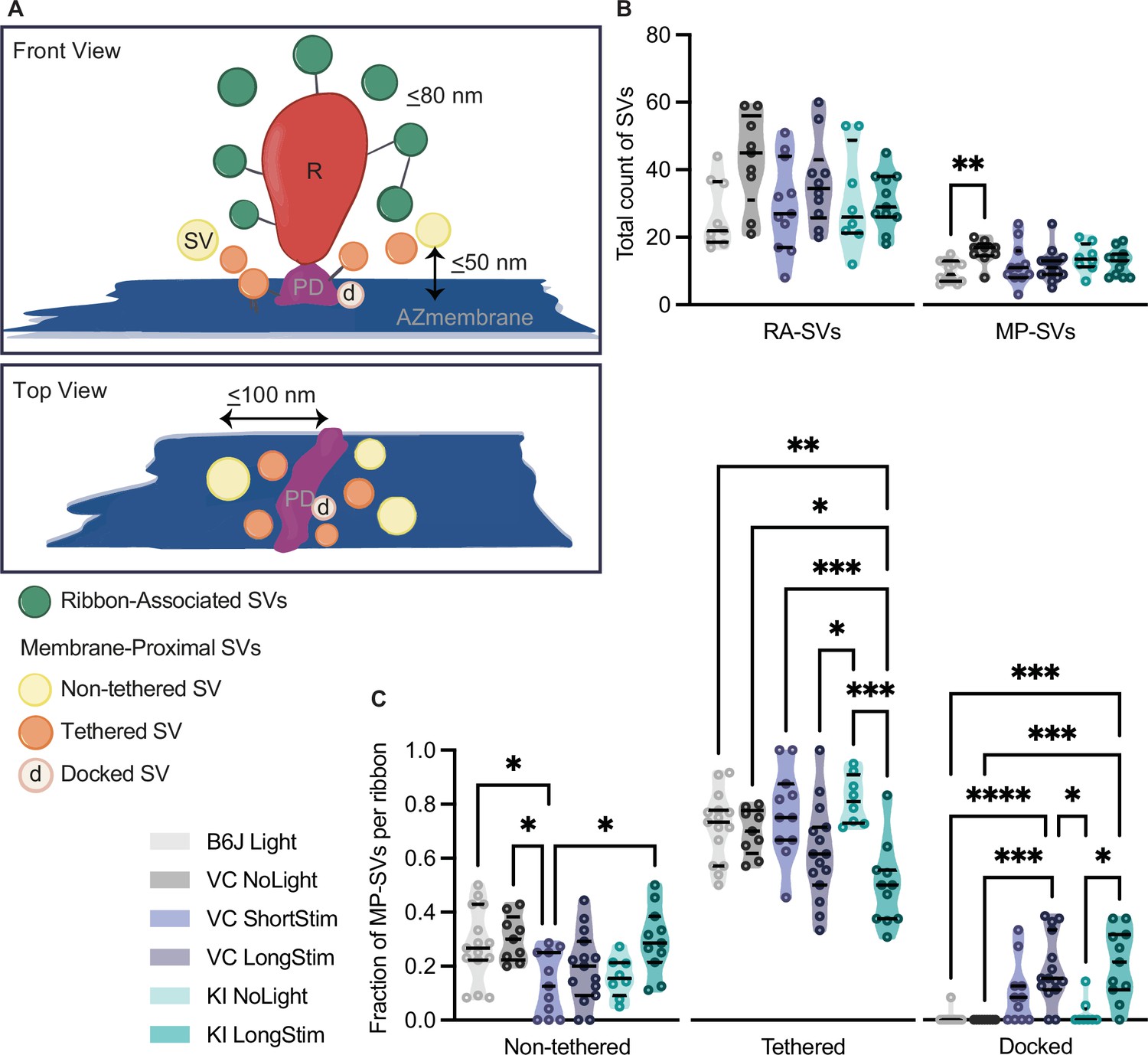
Analysis of morphologically defined vesicle pools for each genotype.
(A) Schematic illustration of a ribbon synapse (not drawn to scale) showing the parameters taken into account for the analysis of the different vesicle pools. Membrane-proximal (MP)-synaptic vesicles (SVs) constitute the first row of vesicles within 50 nm membrane-to-membrane distance from the active zone (AZ) membrane (blue) and 100 nm from the presynaptic density (PD, pink). Docked SVs are defined as vesicles in a distance of 0–2 nm to the AZ membrane. Non-tethered SVs are in yellow, tethered in orange, and docked in light pink. For ribbon-associated (RA)-SVs, vesicles (green) within 80 nm from the ribbon (R, in red) are included. (B) Total count of SVs per pool (RA- and MP-SV pools), per ribbon. (C) Fraction of non-tethered, tethered, and docked MP-SVs per ribbon for the controls as well as for Ai32VC ShortStim, Ai32VC LongStim, and Ai32KI LongStim. Data are presented in mean ± SEM. *p<0.05, **p<0.01, ***p<0.001, and ****p<0.0001. Statistical test: one-way ANOVA followed by Tukey’s test (parametric data) and Kruskal-Wallis (KW) test followed by Dunn’s test (non-parametric data). MP-SV pool: B6J LongStim: nribbons = 15, Nanimals = 2. Ai32VC NoLight: nribbons = 9, Nanimals = 2. Ai32VC ShortStim: nribbons = 11, Nanimals = 1. Ai32VC LongStim: nribbons = 15, Nanimals = 2. Ai32KI NoLight: nribbons = 8, Nanimals = 2. Ai32KI LongStim: nribbons = 11, Nanimals = 2. RA-SV pool: B6J LongStim: nribbons = 9, Nanimals = 1. Ai32VC NoLight: nribbons = 9, Nanimals = 2. Ai32VC ShortStim: nribbons = 11, Nanimals = 1. Ai32VC LongStim: nribbons = 10, Nanimals = 1. Ai32KI NoLight: nribbons = 8, Nanimals = 2. Ai32KI LongStim: nribbons = 11, Nanimals = 2.
Figure 6—figure supplement 2
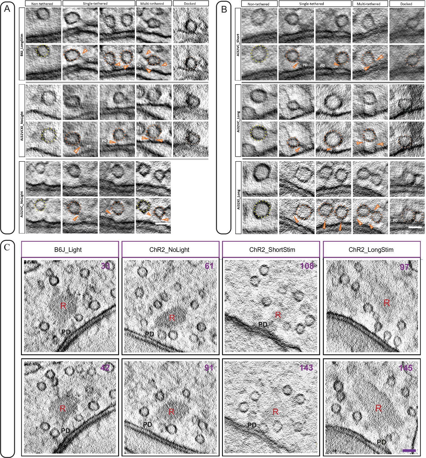
Different morphological sub-pools within the membrane-proximal (MP) pool at ribbon synapse active zone (AZ).
(A) Representative tomogram virtual sections show different morphological synaptic vesicle (SV) sub-pools in the MP-SV pool in our control conditions. Docked SVs are rare and for Ai32VC animals docked SVs were not observed in our no light control data set. (B) Representative examples showing different MP-SV morphological sub-pools upon short (upper panel) and long (middle and lower panel) light stimulation. The non-tethered SVs are in yellow dotted lines, single-tethered to the PD by arrowheads and docked SVs with peach dotted lines. (C) Depicted are additional virtual sections for each condition. The virtual section number is indicated in the upper right corner, the presynaptic density with PD and the ribbon with R. Scale bar in A, B, and C: 50 nm.
Figure 7 with 2 supplements
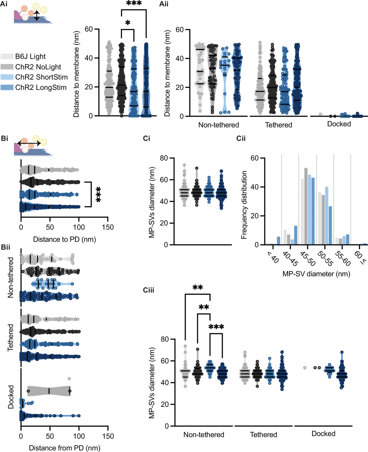
Membrane-proximal (MP)-synaptic vesicles (SVs) come closer to the active zone (AZ) membrane and the presynaptic density upon light stimulation.
(Ai) MP-SVs distance to the AZ membrane. (Aii) Distance of the sub-pools to the AZ membrane. (Bi) MP-SVs distance to the PD. (Bii) Distance of the sub-pools to the PD. (Ci) Diameter of MP-SVs quantified from the outer rim to the outer rim. (Cii) Frequency distribution of SV diameter of all MP-SVs. (Ciii) SV diameters of the sub-pools. Data are presented in mean ± SEM. *p<0.05, **p<0.01, ***p<0.001, and ****p<0.0001. Statistical test: one-way ANOVA followed by Tukey’s test (parametric data) and Kruskal-Wallis (KW) test followed by Dunn’s test (non-parametric data). B6J Light: nribbons = 15, nsv = 146, Nanimals = 2. ChR2 NoLight: nribbons = 17, nsv = 253, Nanimals = 4. ChR2 ShortStim: nribbons = 11, nsv = 132, Nanimals = 1. ChR2 LongStim: nribbons = 26, nsv = 311, Nanimals = 4.
Figure 7—figure supplement 1
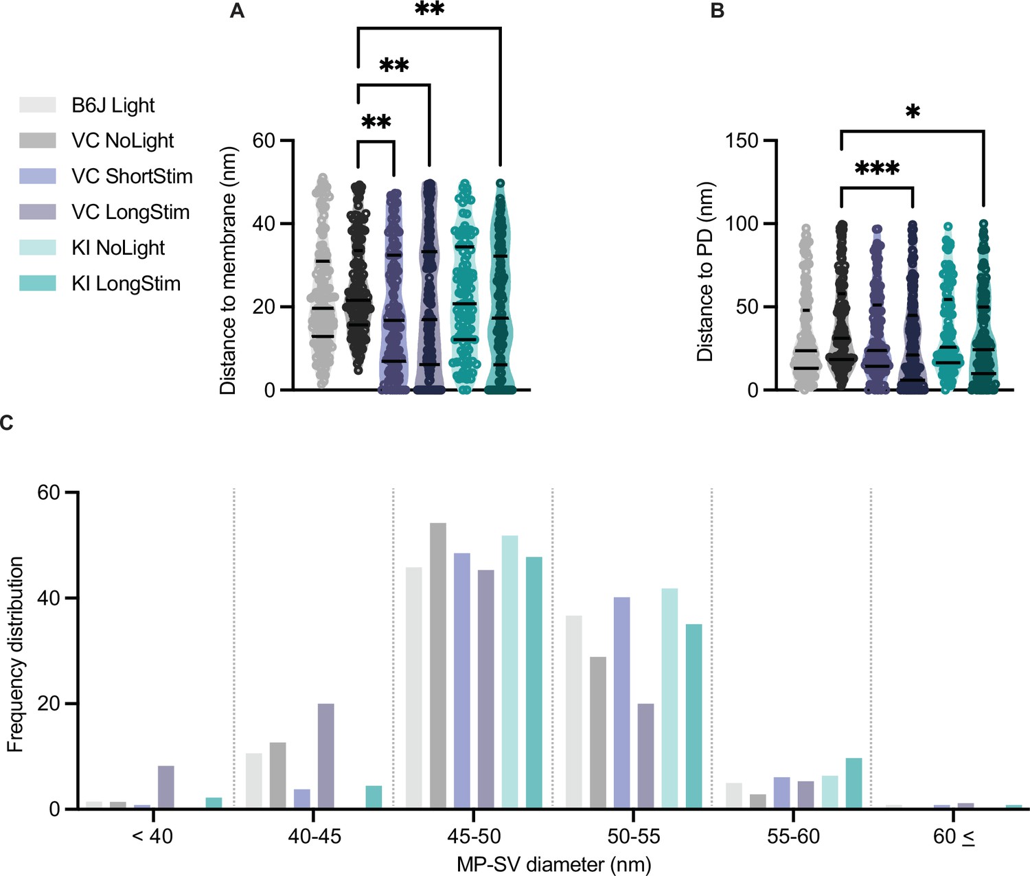
Distances of membrane-proximal (MP)-synaptic vesicles (SVs) to the active zone (AZ) membrane and the presynaptic density as well as their diameters.
(A) MP-SVs distance to the AZ membrane. (B) MP-SVs distance to the PD. (C) Frequency distribution of SV diameter of all MP-SVs. Data are presented in mean ± SEM. *p<0.05, **p<0.01, ***p<0.001, and ****p<0.0001. Statistical test: one-way ANOVA followed by Tukey’s test (parametric data) and Kruskal-Wallis (KW) test followed by Dunn’s test (non-parametric data). B6J LongStim: nribbons = 15, nsv = 146, Nanimals = 2. Ai32VC NoLight: nribbons = 9, nsv = 142, Nanimals = 2. Ai32VC ShortStim: nribbons = 11, nsv = 132, Nanimals = 1. Ai32VC LongStim: nribbons = 15, nsv = 174, Nanimals = 2. Ai32KI NoLight: nribbons = 8, nsv = 111, Nanimals = 2. Ai32KI LongStim: nribbons = 11, nsv = 137, Nanimals = 2.
Figure 7—figure supplement 2
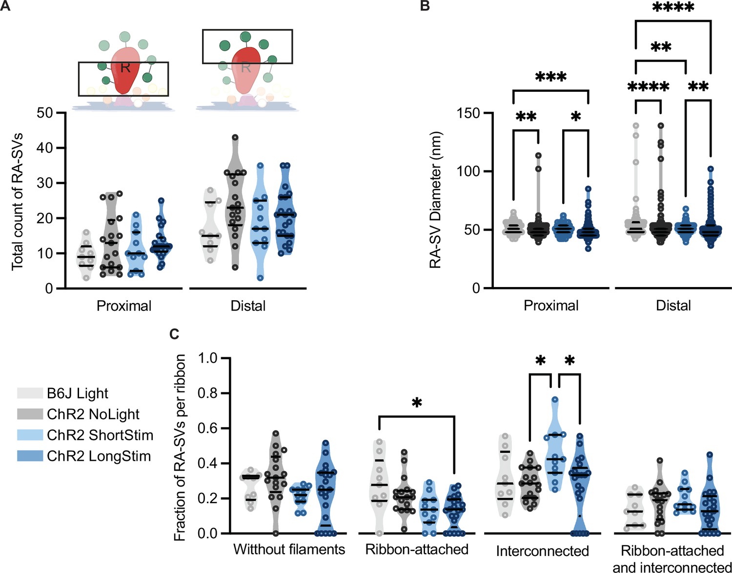
Analysis of morphologically defined ribbon-associated (RA)-synaptic vesicles (SVs).
(A) RA-SVs total count when divided into two ribbon halves – proximal vs. distal. The illustration above highlights the congruent group. (B) The diameter of proximal vs. distal RA-SVs. (C) The fraction of RA-SVs per ribbon divided into SVs without filaments, ribbon-attached, interconnected, and both ribbon-attached and interconnected. Data are presented in mean ± SEM. Statistical test: one-way ANOVA followed by Tukey’s test (parametric data) and Kruskal-Wallis (KW) test followed by Dunn’s test (non-parametric data). Significance is indicated by *p<0.05, **p<0.01, ***p<0.001, and ****p<0.0001. RA-SV pool: B6J LongStim: nribbons = 9, nsv = 238, Nanimals = 1. Ai32VC NoLight: nribbons = 9, nsv = 327, Nanimals = 2. Ai32VC ShortStim: nribbons = 11, nsv = 324, Nanimals = 1. Ai32VC LongStim: nribbons = 10, nsv = 362, Nanimals = 1. Ai32KI NoLight: nribbons = 8, nsv = 249, Nanimals = 2. Ai32KI LongStim: nribbons = 11, nsv = 338, Nanimals = 2.
Figure 8
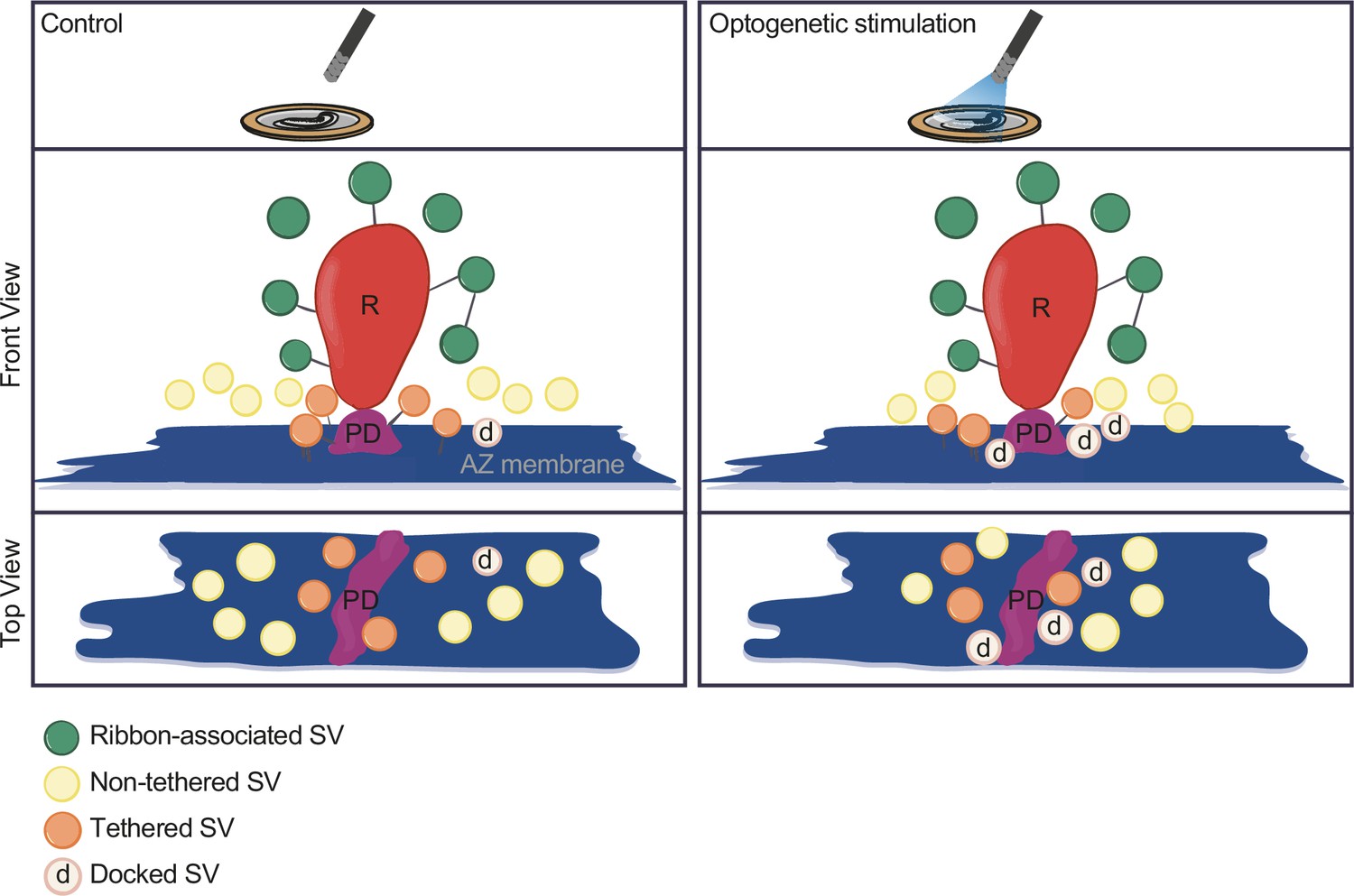
Summary.
Optogenetic stimulation of inner hair cells (IHCs) recruits synaptic vesicles (SVs) more tightly to the active zone (AZ) membrane and potentially closer to the Ca2+ channels. The proportion of docked SVs increased and tethered decreased upon stimulation duration, while the total count of membrane-proximal (MP)-SVs and ribbon-associated (RA)-SVs stayed stable. The distance of MP-SVs to the presynaptic density (PD) slightly decreased upon stimulation.
Author response image 1
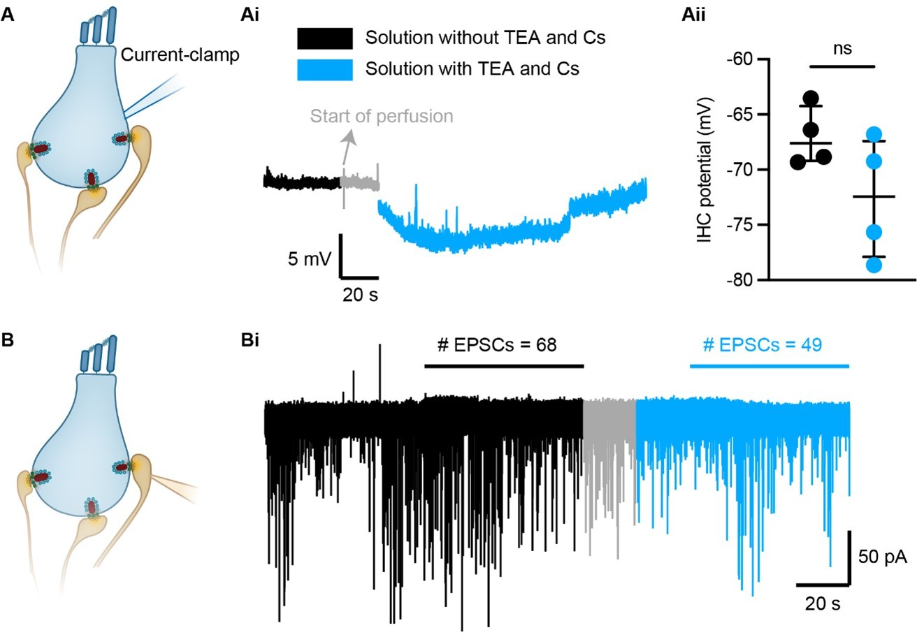
The IHC potential and spontaneous release does not change significantly in the presence of 20 mM TEA and 1mM Cs.
(A) The IHC potential was measured using perforated patch-clamp recordings in current clamp mode. Two different solutions, without and with 20 mM TEA and 1 mM CsCl, were quickly perfused (>100 mL/h) during the recordings. (Ai) The IHC potential was monitored during continuous recordings of 20 s. (Aii) There was no significant change in the IHC potential with the two solutions. The presence of TEA and Cs slightly hyperpolarized the IHC potential by 5.56 ± 1.615 mV (4 cells; p-value = 0.1250, Wilcoxon matched-pairs signed rank test). (B) Spontaneous EPSCs were recorded from individual afferent boutons using continuous ruptured patch-clamp recordings of 20 s. (Bi) We quantified the number of EPSCs occurring during one minute before the start of perfusion and during one minute after the bath solution has been exchanged.
Author response image 2
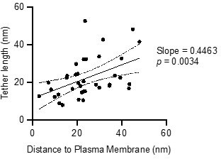
Correlation between tether length and the distance of a tethered SV to the plasma membrane.
Dataset from Chakrabarti et al. 2018, wild type under resting conditions.
Tables
Table 1
Ribbon counts in three different age groups of ChR2-expressing inner hair cells (IHCs) and their WT controls.
Data are presented as mean ± SEM. p-Values are calculated by two-way ANOVA followed by Tukey’s test for multiple comparisons. Results of the comparisons between age groups of the same genotype and between genotypes of the same age group are reported. Significant results are indicated with **p<0.01, ***p<0.001, and ****p<0.0001.
| N animals | N ROIs | ncells | Ribbon count (mean ± SEM) | Age comparison | Genotype comparison | |||
|---|---|---|---|---|---|---|---|---|
| p-Value | Test | p-Value | Test | |||||
| WT G1 | 2 | 12 | 99 | 9.82±0.87 | **, WT G1 vs. WT G3 | ns, WT G1 vs. Ai32KI cre+ G1 | ||
| 0.0077 | Two-way ANOVA | 0.9124 | Two-way ANOVA | |||||
| WT G2 | 2 | 11 | 87 | 7.60±0.99 | ns, WT G2 vs. WT G1 | ns, WT G2 vs. Ai32KI cre+ G2 | ||
| 0.2045 | Two-way ANOVA | 0.1046 | Two-way ANOVA | |||||
| WT G3 | 2 | 11 | 65 | 6.39±0.56 | ns, WT G3 vs. WT G2 | ns, WT G3 vs. Ai32KI cre+ G3 | ||
| 0.8179 | Two-way ANOVA | 0.9689 | Two-way ANOVA | |||||
| Ai32KI cre+ G1 | 3 | 21 | 170 | 8.97±0.48 | ****, Ai32KI cre+ G1 vs. Ai32KI cre+ G2 | |||
| <0.0001 | Two-way ANOVA | |||||||
| Ai32KI cre+ G2 | 2 | 19 | 116 | 5.32±0.43 | ns, Ai32KI cre+ G2 vs. Ai32KI cre+ G3 | |||
| 0.9968 | Two-way ANOVA | |||||||
| Ai32KI cre+ G3 | 2 | 17 | 129 | 5.69±0.42 | ***, Ai32KI cre+ G3 vs. Ai32KI cre+ G1 | |||
| 0.0005 | Two-way ANOVA | |||||||
Table 2
List of membrane-proximal (MP)-synaptic vesicle (SV) parameters showing the mean ± SEM values, N, n, p-values and the statistical tests applied.
Data are presented as mean ± SEM. Data was tested for significant differences by one-way ANOVA followed by Tukey’s test (parametric data) or Kruskal-Wallis (KW) test followed by Dunn’s test (non-parametric data). Significant results are indicated with *p<0.05; **p<0.01; ***p<0.001; and ****p<0.0001.
| B6J Light | ChR2 NoLight | ChR2 ShortStim | ChR2 LongStim | Adjusted p-value | Test | ||
|---|---|---|---|---|---|---|---|
| Nanimals | 2 | 4 | 1 | 4 | |||
| nribbons Total | 15 | 17 | 11 | 26 | |||
| nribbons Ai32VC | 9 | 11 | 15 | ||||
| nribbons Ai32KI | 8 | 0 | 11 | ||||
| nSV Total | 146 | 253 | 132 | 311 | |||
| nSV Non-tethered | 38 | 60 | 20 | 75 | |||
| nSV Tethered | 107 | 191 | 99 | 175 | |||
| nSV Docked | 1 | 2 | 13 | 61 | |||
| MP-SVs count | 9.73 | 14.88 | 12.00 | 11.96 | **; B6J Light vs. ChR2 NoLight | KW test – Dunn’s test | |
| ±0.796 | ±0.935 | ±1.844 | ±0.833 | 0.0028 | |||
| Fraction of non-tethered SVs | 0.28 | 0.23 | 0.14 | 0.24 | *; B6J Light vs. ChR2 ShortStim | ANOVA – Tukey’s test | |
| ±0.035 | ±0.026 | ±0.035 | ±0.026 | 0.0271 | |||
| Fraction of tethered SVs | 0.72 | 0.75 | 0.77 | 0.57 | *; B6J Light vs. ChR2 LongStim | ANOVA – Tukey’s test | |
| ±0.033 | ±0.025 | ±0.049 | ±0.034 | 0.0151 | |||
| ***; ChR2 LongStim vs. ChR2 NoLight | |||||||
| 0.0008 | |||||||
| **; ChR2 LongStim vs. ChR2 ShortStim | |||||||
| 0.002 | |||||||
| Fraction of docked SVs | 0.01 | 0.01 | 0.10 | 0.20 | ****; B6J Light vs. ChR2 LongStim | KW test – Dunn’s test | |
| ±0.006 | ±0.009 | ±0.034 | ±0.025 | <0.0001 | |||
| ****; ChR2 LongStim vs. ChR2 NoLight | |||||||
| <0.0001 | |||||||
| Fraction of tethered | Single PM tethered | 0.25 | 0.30 | 0.18 | 0.25 | n.s. | ANOVA – Tukey’s test |
| ±0.052 | ±0.039 | ±0.055 | ±0.036 | ||||
| Single PD tethered | 0.12 | 0.12 | 0.02 | 0.13 | n.s. | KW test – Dunn’s test | |
| ±0.046 | ±0.029 | ±0.013 | ±0.032 | ||||
| Interconnected | 0.02 | 0.02 | 0.04 | 0.05 | n.s. | KW test – Dunn’s test | |
| ±0.01 | ±0.009 | ±0.023 | ±0.029 | ||||
| Multiple tethered | 0.61 | 0.56 | 0.76 | 0.56 | n.s. | ANOVA – Tukey’s test | |
| ±0.068 | ±0.051 | ±0.048 | ±0.046 | ||||
| Distance to the membrane | All MP-SVs | 22.78 | 23.67 | 19.41 | 19.61 | ***; ChR2 LongStim vs. ChR2 NoLight | KW test – Dunn’s test |
| ±1.08 | ±0.776 | ±1.263 | ±0.876 | 0.0007 | |||
| *; ChR2 NoLight vs. ChR2 ShortStim | |||||||
| 0.0105 | |||||||
| Non-tethered | 32.42 | 31.81 | 31.32 | 30.06 | n.s. | KW test – Dunn’s test | |
| ±2.138 | ±1.655 | ±3.172 | ±1.481 | ||||
| Tethered | 19.56 | 21.36 | 19.51 | 21.94 | n.s. | KW test – Dunn’s test | |
| ±1.077 | ±0.789 | ±1.292 | ±0.982 | ||||
| Docked | 1.44 | 0.00 | 0.34 | 0.09 | Not tested: low n of docked SVs in control and NoLight conditions | ||
| ±0 | ±0 | ±0.18 | ±0.053 | ||||
| Distance to the PD | All MP-SVs | 31.88 | 37.61 | 32.96 | 30.13 | ***; ChR2 LongStim vs. ChR2 NoLight | KW test – Dunn’s test |
| ±2.144 | ±1.622 | ±2.192 | ±1.509 | 0.0001 | |||
| Non-tethered | 35.49 | 47.09 | 45.34 | 38.07 | 0.0502 | KW test – Dunn’s test | |
| ±4.386 | ±3.321 | ±3.654 | ±3.124 | ||||
| Tethered | 30.12 | 34.52 | 34.12 | 31.49 | n.s. | KW test – Dunn’s test | |
| ±2.426 | ±1.808 | ±2.571 | ±1.975 | ||||
| Docked | 83.27 | 48.46 | 5.06 | 16.43 | Not tested: low n of docked SVs in control and NoLight conditions | ||
| ±0 | ±35.88 | ±1.892 | ±2.876 | ||||
| Diameter of SVs | All MP-SVs | 49.00 | 48.67 | 49.17 | 48.05 | KW test – Dunn’s test | |
| ±0.442 | ±0.25 | ±0.352 | ±0.303 | ||||
| Non-tethered | 50.17 | 49.71 | 53.27 | 48.76 | **; B6J Light vs. ChR2 ShortStim | KW test – Dunn’s test | |
| ±1.061 | ±0.63 | ±0.835 | ±0.485 | 0.0093 | |||
| ***; ChR2 LongStim vs. ChR2 ShortStim | |||||||
| 0.0004 | |||||||
| **; ChR2 NoLight vs. ChR2 ShortStim | |||||||
| 0.0069 | |||||||
| Tethered | 48.55 | 48.29 | 48.06 | 47.76 | n.s. | KW test – Dunn’s test | |
| ±0.465 | ±0.259 | ±0.359 | ±0.419 | ||||
| Docked | 53.70 | 53.70 | 51.29 | 47.97 | Not tested: low n of docked SVs in control and NoLight conditions | ||
| ±0 | ±0 | ±0.845 | ±0.773 | ||||
Table 3
Comparison of the number of docked synaptic vesicles (SVs) from different studies under different stimulation paradigms.
| Condition/genotype | Publication | Number of tomograms | Average number of docked SVs/AZ | Total number of docked SVs |
|---|---|---|---|---|
| BL6 Light | This study | 15 | 0.07 | 1 |
| ChR2 NoLight | This study | 17 | 0.12 | 2 |
| ChR2 ShortStim | This study | 11 | 1.18 | 13 |
| ChR2 LongStim | This study | 26 | 2.35 | 61 |
| BL6 rest | Chakrabarti et al., 2018 | 7 | 0.14 | 1 |
| BL6 potassium stim | Chakrabarti et al., 2018 | 10 | 0.4 | 4 |
| BL6 rest | Kroll et al., 2020 | 10 | 0.2 | 2 |
| BL6 potassium stim | Kroll et al., 2020 | 9 | 0.22 | 2 |
Key resources table
| Reagent type (species) or resource | Designation | Source or reference | Identifiers | Additional information |
|---|---|---|---|---|
| Strain, strain background (Mus musculus) | Vglut3-Cre (VC) | Jung et al., 2015b; Vogl et al., 2016 | PMID:26034270 PMID:27458190 | Coding sequence for Cre inserted in start codon of Vglut3/Slc17a8 gene on BAC RP24-88H21 |
| Strain, strain background (Mus musculus) | Vglut3-Ires-Cre-KI (KI) | Lou et al., 2013; Vogl et al., 2016 | PMID:23325226; PMID:27458190 | Knock in of ires-Cre cassette 3 |
| Strain, strain background (Mus musculus) | B6.Cg-Gt(ROSA)26Sortm32(CAG-COP4*H134R/EYFP)Hze/J, common name: Ai32 | Madisen et al., 2012 | Strain #:024109, RRID: IMSR_JAX:024109 | |
| Strain, strain background (Mus musculus) | C57BL/6J | Jackson Laboratory | Strain #: 000664 RRID:IMSR_JAX:000664 | |
| Antibody | Chicken anti-GFP (polyclonal) | Abcam | Cat. #: ab13970; RRID: AB_300798 | IF; Concentrations used: 1:500 |
| Antibody | Rabbit anti-myo6 (polyclonal) | Proteus Biosciences | Cat. #: 25–6791; RRID: AB_10013626 | IF; Concentrations used: 1:200 |
| Antibody | Mouse anti-CtBP2 (monoclonal) | BD Biosciences | Cat. #: 612044; RRID: AB_399431 | IF; Concentrations used: 1:200 |
| Antibody | Mouse anti-neurofilament 200 (monoclonal) | Sigma | Cat. #: N5389; RRID: AB_260781 | IF; Concentrations used: 1:400 |
| Antibody | Rabbit anti-Vglut3 (polyclonal) | SySy | Cat. #: 135 203; RRID: AB_887886 | IF; Concentrations used: 1:300 |
| Antibody | Goat anti-chicken Alexa Fluor 488 (polyclonal) | Invitrogen | Cat. #: A11039; RRID: AB_2534096 | IF; Concentrations used: 1:200 |
| Antibody | AbberiorStar 580 goat-conjugated anti-rabbit (polyclonal) | Abberior | Cat. #: 2-0012-005-8; RRID: AB_2810981 | IF; Concentrations used: 1:200 |
| Antibody | AbberiorStar 635p goat-conjugated anti-mouse (polyclonal) | Abberior | Cat. #: 2-0002-007-5; RRID: AB_2893232 | IF; Concentrations used: 1:200 |
| Antibody | Goat anti-mouse Alexa Fluor 647 (polyclonal) | Invitrogen | Cat. #: A-21236; RRID: AB_2535805 | IF; Concentrations used: 1:200 |
| Antibody | Goat anti-rabbit Alexa Fluor 568 (unknown) | Thermo Fisher | RRID: AB_143157 | IF; Concentrations used: 1:200 |
| Sequence-based reagent | Ai32 recombinant_foward | This paper | PCR primers | 5’ – GTGCTGTC TCATCATTTTGGC – 3 |
| Sequence-based reagent | Ai32 recombinant_reverse | This paper | PCR primers | 5’ – TCCATAATCCATGGTGGCAAG – 3 |
| Sequence-based reagent | CGCT recombinant_foward | This paper | PCR primers | 5’ – CTGCTAACCATGTTCATGCC – 3‘ |
| Sequence-based reagent | CGCT recombinant_reverse | This paper | PCR primers | 5’ – TTCAGGGTCAGCTTGCCGTA – 3‘ |
| Software, algorithm | Patchers Power Tools | Igor Pro XOP (http://www3.mpibpc.mpg.de/groups/neher/index.php?page=software) | RRID: SCR_001950 | |
| Software, algorithm | ImageJ software | ImageJ (http://imagej.nih.gov/ij/) | RRID: SCR_003070 | |
| Software, algorithm | Fiji software | Fiji (http://fiji.sc) | RRID: SCR_002285 | |
| Software, algorithm | Imaris | Oxford Instruments (http://www.bitplane.com/imaris/imaris) | RRID:SCR_007370 | |
| Software, algorithm | Excel | Microsoft (https://microsoft.com/mac/excel) | RRID:SCR_016137 | |
| Software, algorithm | GraphPad Prism software | GraphPad Prism (https://graphpad.com) | RRID:SCR_002798 | |
| Software, algorithm | Igor Pro software package | Wavemetrics (http://www.wavemetrics.com/products/igorpro/igorpro.htm) | RRID: SCR_000325 | |
| Software, algorithm | SerialEM | Mastronarde, 2005 (https://bio3d.colorado.edu/SerialEM/) | PMID:16182563 | |
| Software, algorithm | 3dmod | Kremer et al., 1996 (https://bio3d.colorado.edu/imod/doc/3dmodguide.html) | PMID:8742726 | |
| Software, algorithm | IMOD | http://bio3d.colorado.edu/imod | RRID: SCR_003297 | Generating tomograms using the ‘etomo’ GUI of IMOD |
| Software, algorithm | Gatan Microscopy Suite | http://www.gatan.com/products/tem-analysis/gatan-microscopy-suite-software | RRID: SCR_014492 | Digital micrograph scripting |
| Software, algorithm | Patchmaster or Pulse | HEKA Elektronik, (http://www.heka.com/products/products_main.html#soft_pm) | RRID: SCR_000034 | |
| Software, algorithm | MATLAB | http://www.mathworks.com/products/matlab/ | RRID: SCR_001622 | |
| Others | IMARIS routine: Source code 1 | This paper | N/A | To analyze the number of ribbons per IHC. Related to Figure 1D |
| Others | IgorPro routine: OptoEPSCs (Source code 2) | This paper | N/A | For light-evoked EPSCs. Related to Figure 4C–F |
| Others | MATLAB routine: HPMacquire (Source code 3) | This paper | N/A | To control light pulse for Opto-HPF in a computer interface. Related to Figure 3A |
| Others | MATLAB routine: Intensityprofilecalculator (Source code 4) | This paper | N/A | For irradiance analysis. Related to Figure 3E |
| Others | MATLAB routine: HPManalyse (Source code 5) | This paper | N/A | For sensor data alignment. Related to Figure 5C |
Table 4
Genotypes, animal numbers, as well as the ages of the animals used in the experiments.
| Experiment | Genotype | Nanimals | n (cells/ribbon) | Age |
|---|---|---|---|---|
| Immunohistochemistry | Ai32KI cre+ | 3 | 170 cells | Group 1: 4–5 months |
| Ai32KI cre+ | 2 | 116 cells | Group 2: 6–7 months | |
| Ai32KI cre+ | 2 | 129 cells | Group 3: 9–12 months | |
| Immunohistochemistry | WT | 2 | 99 cells | Group 1: 4–5 months |
| WT | 2 | 87 cells | Group 2: 6–7 month | |
| WT | 2 | 65 cells | Group 3: 9–12 months | |
| Pre-embedding immunogold | Ai32KI cre+ | 1 | P17 | |
| Patch-clamp | Ai32VC cre+(fl/fl) | 7 | 17 cells | P14-17 |
| Ai32VC cre+(fl/+) | 5 | 5 cells | P14-17 | |
| Ai32KI cre+ | 3 | 21 cells | P16-20 | |
| Electron tomography MP-SVs | P14-20 | |||
| ShortStim | Ai32VC cre+ | 1 | 11 ribbons | |
| LongStim | Ai32VC cre+ | 2 | 15 ribbons | |
| LongStim | B6J | 2 | 15 ribbons | |
| LongStim | Ai32KI cre+ | 2 | 11 ribbons | |
| NoLight | Ai32VC cre+ | 2 | 9 ribbons | |
| NoLight | Ai32KI cre+ | 2 | 8 ribbons | |
| Electron tomography RA-SVs | P14-20 | |||
| ShortStim | Ai32VC cre+ | 1 | 11 ribbons | |
| LongStim | Ai32VC cre+ | 1 | 10 ribbons | |
| LongStim | B6J | 1 | 9 ribbons | |
| LongStim | Ai32KI cre+ | 2 | 11 ribbons | |
| NoLight | Ai32VC cre+ | 2 | 9 ribbons | |
| NoLight | Ai32KI cre+ | 2 | 8 ribbons |
Additional files
-
Supplementary file 1
List of clathrin-coated (CC) structures at the active zone (AZ).
Statistics could not be performed due to the rare abundance of CC structures at the AZ in our tomograms. The gray columns indicate CC structures intermingled with the membrane-proximal (MP)-synaptic vesicle (SV) pool.
- https://cdn.elifesciences.org/articles/79494/elife-79494-supp1-v2.docx
-
Supplementary file 2
List of ribbon-associated (RA)-synaptic vesicle (SV) parameters showing the mean ± SEM values, N, n, p-values and the statistical tests applied.
Data are presented as mean ± SEM. Data was tested for significant differences by one-way ANOVA followed by Tukey’s test (parametric data) or Kruskal-Wallis (KW) test followed by Dunn’s test (non-parametric data). Significant results are indicated with *p<0.05; **p<0.05; and ****p<0.0001.
- https://cdn.elifesciences.org/articles/79494/elife-79494-supp2-v2.docx
-
Supplementary file 3
Cutting planes of the analyzed ribbon synapses for each condition.
For each ribbon, we determined the cutting plane and classified it as either a cross-section, a longitudinal section, or a section in between both.
- https://cdn.elifesciences.org/articles/79494/elife-79494-supp3-v2.docx
-
Supplementary file 4
The range of virtual sections per condition.
To judge the size of the tomograms for each condition, we determined the number (and percentage) of tomograms with virtual sections in the most frequent range of 140–170. This range is usually around 50% for all conditions.
- https://cdn.elifesciences.org/articles/79494/elife-79494-supp4-v2.docx
-
MDAR checklist
- https://cdn.elifesciences.org/articles/79494/elife-79494-mdarchecklist1-v2.pdf
-
Source code 1
IMARIS custom plug-ins for the analysis of Figure 1D.
- https://cdn.elifesciences.org/articles/79494/elife-79494-code1-v2.zip
-
Source code 2
Igor Pro custom-written analysis (OptoEPSCs) of light-evoked excitatory postsynaptic currents (EPSCs) related to Figure 4C–F.
- https://cdn.elifesciences.org/articles/79494/elife-79494-code2-v2.zip
-
Source code 3
MATLAB scripts (HPMacquire) for the computer interface to control the light pulse for Opto-HPF.
Related to Figure 3A.
- https://cdn.elifesciences.org/articles/79494/elife-79494-code3-v2.zip
-
Source code 4
MATLAB script (Intensityprofilecalculator) for the analysis of the irradiance in Figure 3E.
- https://cdn.elifesciences.org/articles/79494/elife-79494-code4-v2.zip
-
Source code 5
MATLAB scripts (HPManalyse) for the alignment of the data obtained from the Opto-HPF sensors.
Related to Figure 5C.
- https://cdn.elifesciences.org/articles/79494/elife-79494-code5-v2.zip
Download links
A two-part list of links to download the article, or parts of the article, in various formats.
Downloads (link to download the article as PDF)
Open citations (links to open the citations from this article in various online reference manager services)
Cite this article (links to download the citations from this article in formats compatible with various reference manager tools)
Optogenetics and electron tomography for structure-function analysis of cochlear ribbon synapses
eLife 11:e79494.
https://doi.org/10.7554/eLife.79494


