Figures and data in Emergence of planar cell polarity from the interplay of local interactions and global gradients | eLife

Figures
Additional files

10 figures and 1 additional file

Figures

Figure 1

Download asset Open asset

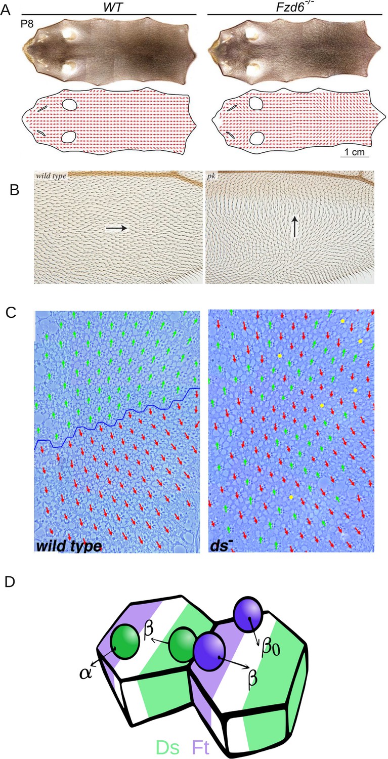
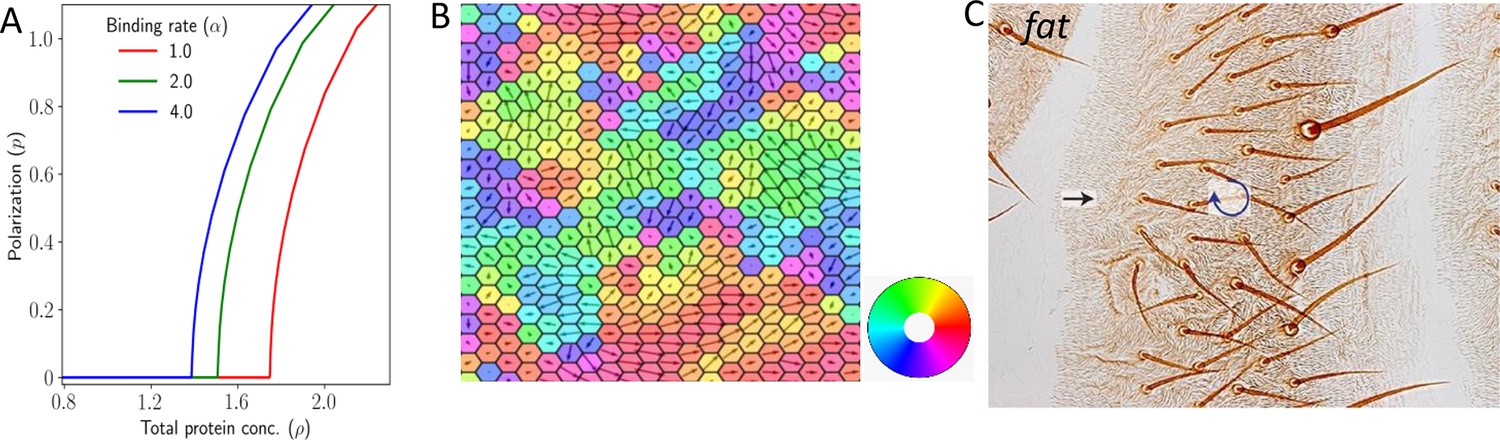
Introduction to planar cell polarity and the model.

Examples of PCP and its disruption in (A) mouse skin (reproduced from Figure 3A of Dong et al., 2018), (B) Drosophila melanogaster wing (reproduced from Figure 4G and H of Ambegaonkar and Irvine, 2015), and (C) Drosophila melanogaster eye leading to irregular ommatidial arrangement (reproduced from Figure S1A and B of Simon, 2004). In (C), green and red arrows represent ommatidial orientation. The blue line indicates the equator. (D) Schematic depicting the protein binding, unbinding kinetics, and heterodimer formation in a two-cell system. Ft (purple bead) and Ds (green bead) bind to the membrane with rate α and unbind with rate $β_{0}$ . The unbinding rate is reduced to $β$ if a heterodimer is formed by the presence of both proteins on the membrane. The green and purple shaded regions indicate higher concentrations of Ft and Ds at the cell membrane, respectively.

© 2018, The Company of Biologists Ltd. Panel A was reproduced from Figure 3A of Dong et al., 2018, with permission from The Company of Biologists Ltd.; permission conveyed through Copyright Clearance Center, Inc. It is not covered by the CC-BY 4.0 license and further reproduction of this panel would need permission from the copyright holder

© 2004, The Company of Biologists Ltd. Panel C was reprinted from Figure S1 A and B of Simon, 2004, with permission from The Company of Biologists Ltd.; permission conveyed through Copyright Clearance Center, Inc. It is not covered by the CC-BY 4.0 license and further reproduction of this panel would need permission from the copyright holder.

Figure 2 with 2 supplements

Download asset Open asset

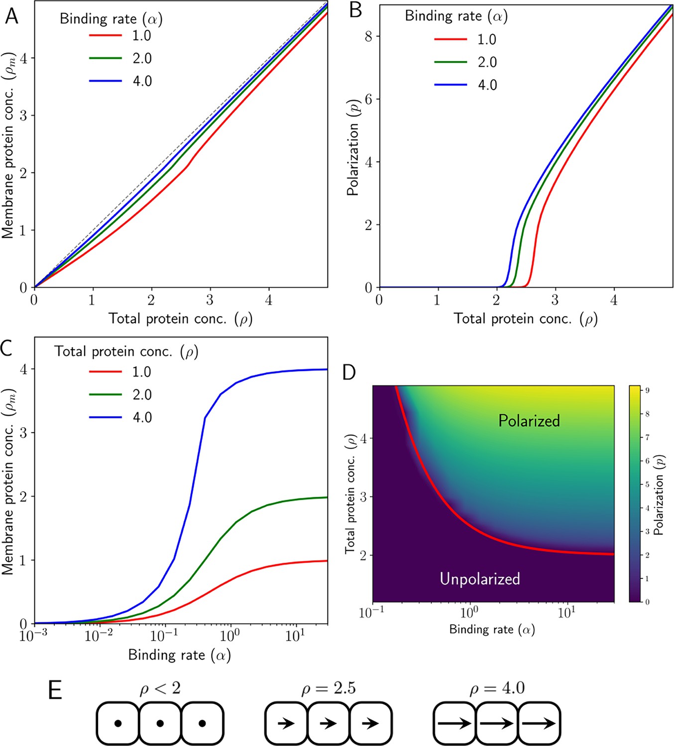
Emergence of polarity due to intercellular protein interactions in 1D.

(A) Membrane protein concentration of Ft and Ds ( $ρ_{m}$ ), and (B) polarization magnitude ( $p$ ) at the steady state against total protein concentration ( $ρ$ ). (C) Membrane protein concentration ( $ρ_{m}$ ) at steady state as a function of protein binding rate ( $α$ ) at different total protein concentrations ( $ρ$ ). (D) Phase diagram of polarization ( $p$ ) as a function of $α$ $ρ$ shows the existence of a polarized and unpolarised state. The red curve in (D) depicts the analytically obtained critical value in Equation 29. (E) Schematic representing cell polarization for different values of $ρ$ . Here, arrows represent the direction and magnitude of cell polarity.

Figure 2—figure supplement 1

Download asset Open asset

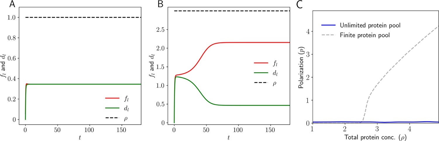
Dynamics in 1D: Level of Ft and Ds in the left and right side ( $f_{l}$ , $f_{r}$ , $d_{l}$ and $d_{r}$ ) of the tissue as a function of time.

(A) When the total protein concentration of Ft and Ds ( $ρ$ ) is below the critical value both proteins localize equally on both sides of the cell. (B) But when the total protein concentration of Ft and Ds ( $ρ$ ) is above the critical value, we observe that the proteins localize completely to one side of the tissue. (C) Membrane protein concentration and Polarization as a function of total protein concentration for the case where cells have an infinite pool of PCP proteins.

Figure 2—figure supplement 2

Download asset Open asset

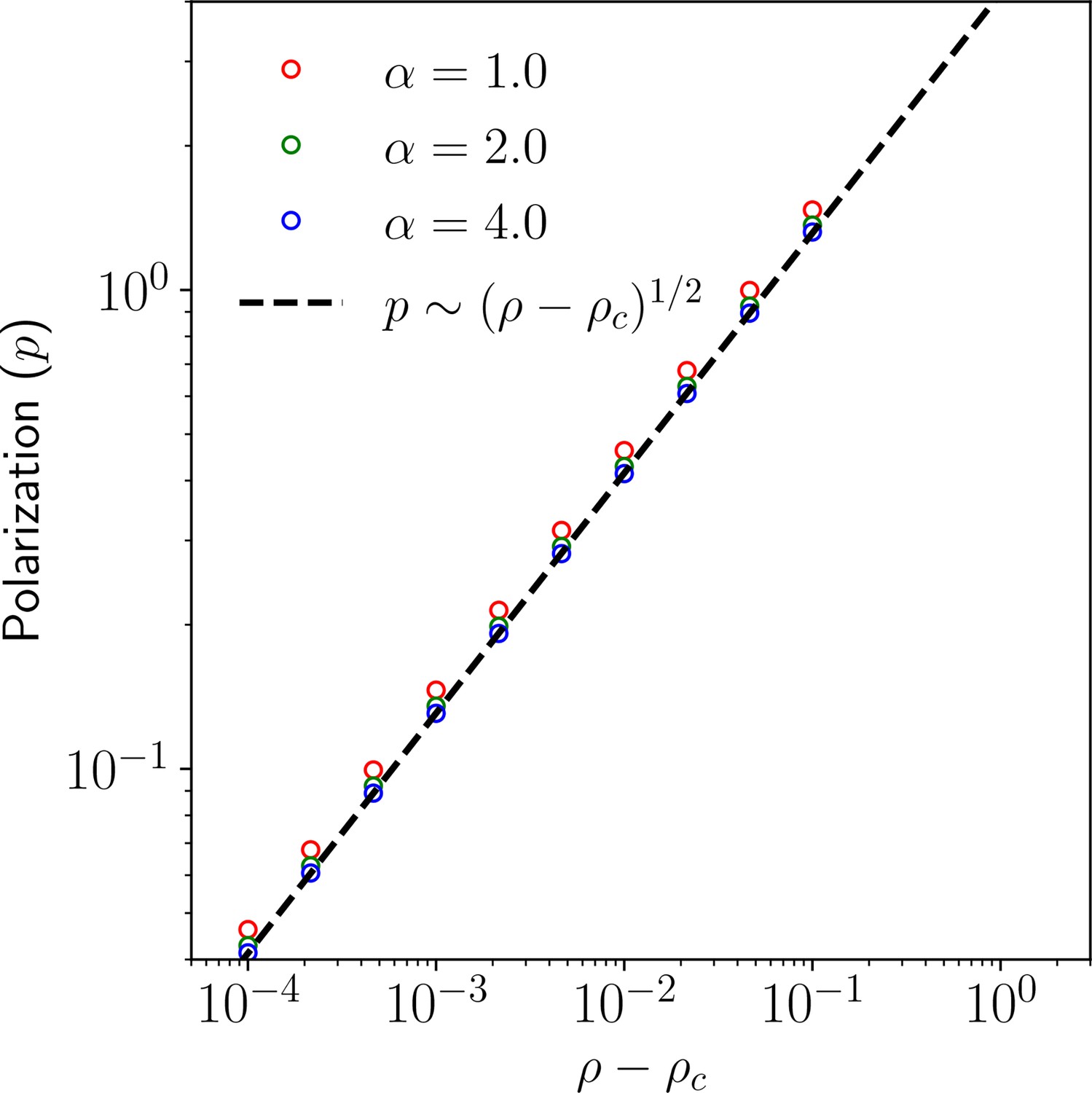
Polarization magnitude as a function of $Δ ρ = ρ - ρ_{c}$ for 1D.

Figure 3 with 1 supplement

Download asset Open asset

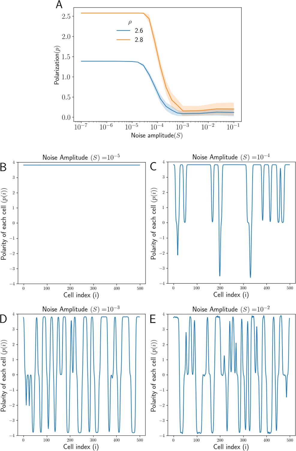
Effect of noise in total protein concentrations on polarization.

(A) Tissue Polarization $p$ as a function of noise $S$ for different values of mean protein levels $ρ$ . The shaded regions mark the standard deviations across the 50 simulations. (B–E) The polarity of each cell $p (i)$ in the tissue for four representative values of noise $S$ . For an increase in the noise in the protein levels, cells form patches of opposing polarizations, resulting in the loss of overall tissue polarity.

Figure 3—figure supplement 1

Download asset Open asset

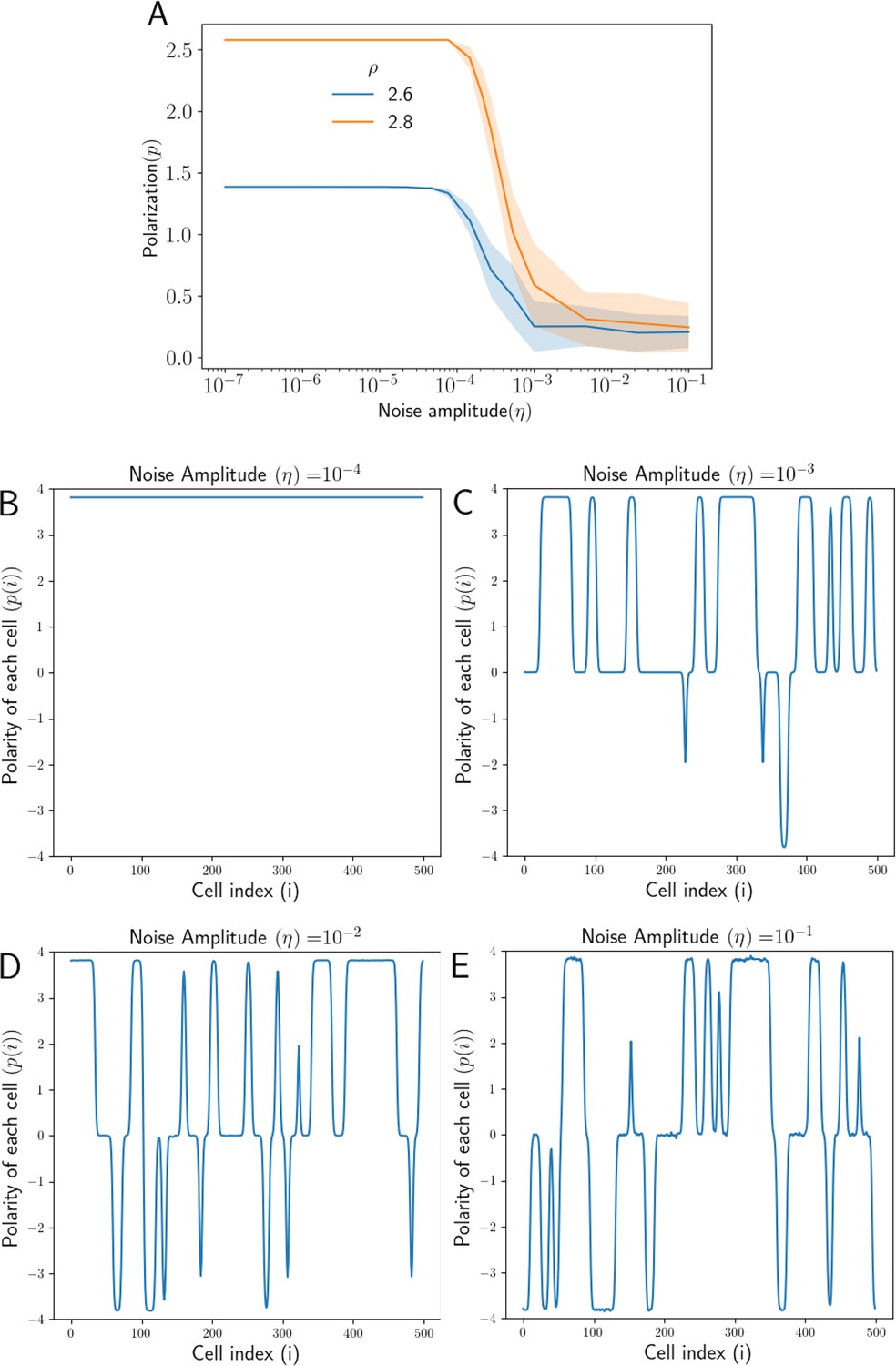
Effect of noise in protein kinetics on polarization.

(A) Overall Polarization ( $p$ ) as function of noise amplitude ( $η$ ) for different total protein concentrations ( $ρ$ ). (B) Polarity of each cell ( $p (i)$ ) in the tissue when the level of noise is negligible ( $10^{- 4}$ ). (C) Polarity of each cell ( $p (i)$ ) at a high amplitude of noise ( $η = 10^{- 3}$ ), some parts of the tissue are aligned in the opposite direction (D) At higher noise amplitude ( $η = 10^{- 2}$ ), the average polarity of the tissue reduces (E) At very high noise amplitude ( $η = 10^{- 1}$ ), the tissue loses overall polarization as different parts of the tissue are aligned in opposite directions.

Figure 4 with 4 supplements

Download asset Open asset

Polarization in 2D lattice in the absence of expression gradient.

(A) Polarization magnitude $| 𝐩 |$ as a function of total protein concentration $ρ$ . (B) A representative example of tissue polarization in the presence of static noise with $S = 10^{- 4}$ . (C) Experimental image showing swirling patterns in case of Ft mutants in Drosophila wing (reproduced from Figure 10A of Ambegaonkar and Irvine, 2015).

Figure 4—figure supplement 1

Download asset Open asset

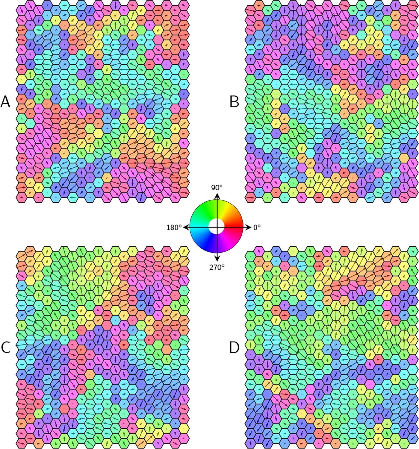
PCP patterns in the presence of static noise.

Four representative examples (A-D) of steady-state polarity patterns in the tissue for uniform protein expression levels with some static noise $S = 0.1$ .

Figure 4—figure supplement 2

Download asset Open asset

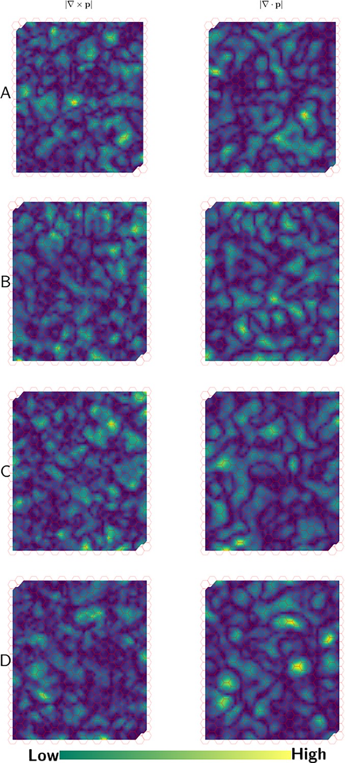
Quantification of asters and swirls in PCP.

(A-D) Magnitude of curl and divergence of the PCP field for the cases shown in Figure 4—figure supplement 1. High magnitudes of curl and divergence denote the centers of swirls and asters, respectively.

Figure 4—video 1

Download asset

posterframe for video — Time evolution videos of non-uniform polarization in 2D without gradient.

We added a static (time-independent) spatial noise to the total protein concentration. Swirling patterns and vortices are formed in the tissue.

Figure 4—video 2

Download asset

posterframe for video — Time evolution videos of polarization when additive white noise has been added to the protein kinetics equations.

We observe that the tissue gets polarized in a non-homogenous manner, and the polarization fluctuates over time.

Figure 5

Download asset Open asset

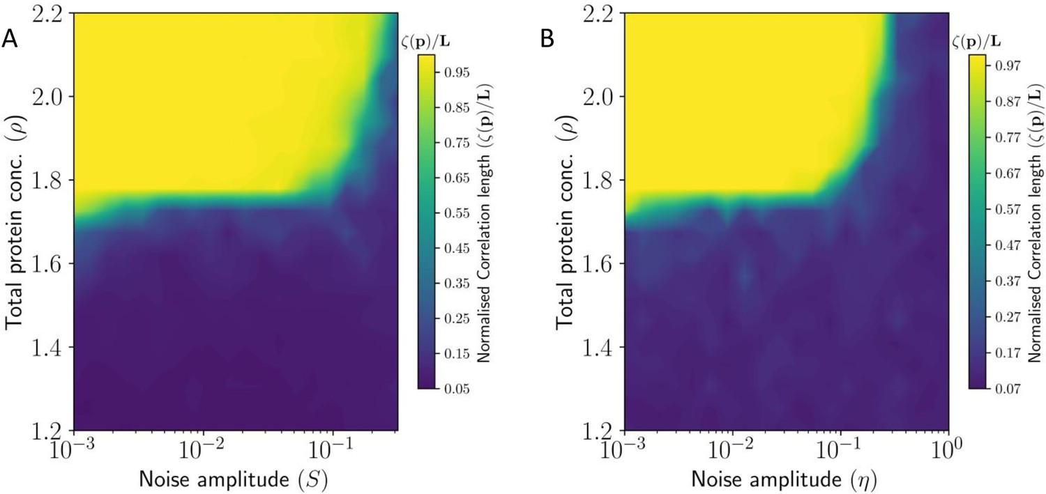
Heat Map showing correlation length $ζ$ of PCP in tissue as a function (A) static noise $S$ , and (B) dynamic noise $η$ , and total protein concentration $ρ$ .

Here the correlation length has been normalized by the system size $L$ .

Figure 6 with 1 supplement

Download asset Open asset

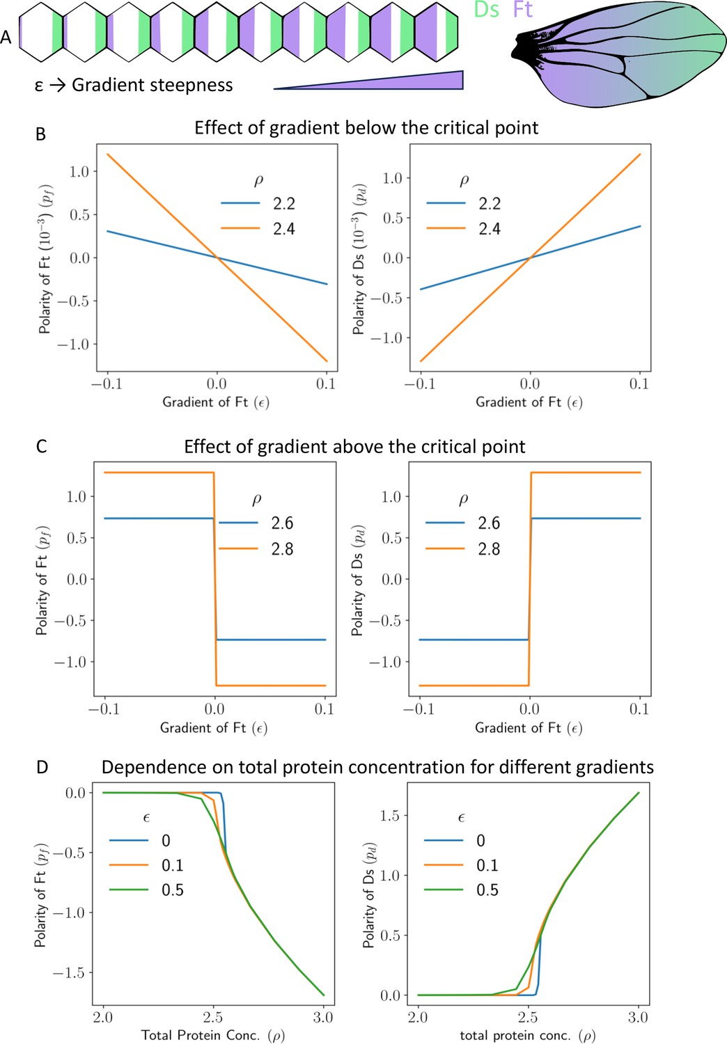
Gradient can polarize the tissue and decide its direction.

(A) Schematics showing expression gradient of Ft in 1D model (left), and an example Drosophila wing with gradient expression levels. (B) Polarity of Ft ( $p_{F t}$ ) and Ds ( $p_{D s}$ ) as a function of gradient of Ft ( $ϵ$ ), when total protein concentration ( $ρ$ ) is below the critical point. (C) Polarity of Ft ( $p_{F t}$ ) and Ds ( $p_{D s}$ ) as a function of gradient ( $ϵ$ ) when total protein concentration ( $ρ$ ) is above the critical point. (D) Polarity of Ft ( $p_{F t}$ ) and Ds ( $p_{D s}$ ) as a function of total protein concentration ( $ρ$ ) for different values of gradient ( $ϵ$ ).

Figure 6—figure supplement 1

Download asset Open asset

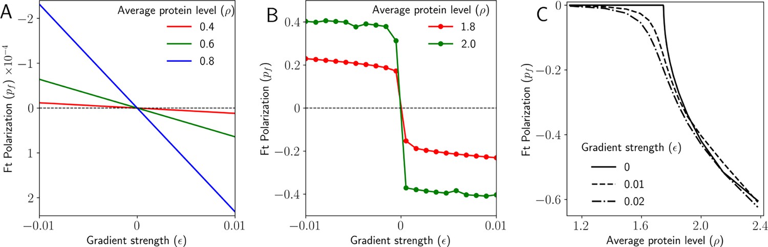
Gradient decides the direction and maintains polarization in 2D.

(A) Polarization of Ft ( $𝐩_{𝐟}$ ) as a function of the gradient of Ft ( $ϵ$ ) when the total protein concentration of Ft and Ds ( $ρ$ ) is below the critical point. (B) Polarization of Ft ( $𝐩_{𝐟}$ ) as a function of the gradient of Ft ( $ϵ$ ) when the total protein concentration of Ft and Ds ( $ρ$ ) is above the critical point. (C) Polarization of Ft ( $𝐩_{𝐟}$ ) as a function of total protein concentration of Ft and Ds ( $ρ$ ) for different values of the gradient of Ft ( $ϵ$ ).

Figure 7 with 1 supplement

Download asset Open asset

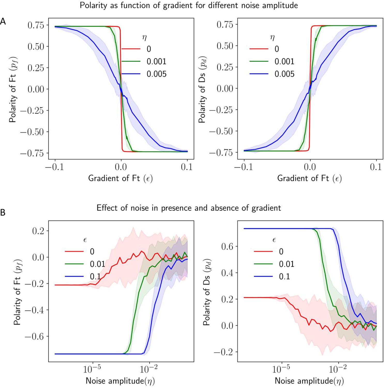
Effect of noise in protein kinetics on the polarization in the presence of gradient cue.

(A) Polarization of Ft ( $p_{f}$ ) and Ds ( $p_{d}$ ) as a function of gradient ( $ϵ$ ) with noise. (B) Polarization of Ft ( $p_{f}$ ) and Ds ( $p_{d}$ ) as a function of noise amplitude ( $η$ ) in the presence of expression gradient. In each panel, the solid lines and the shaded regions mark the average and standard deviations in the polarity over 50 simulations, respectively.

Figure 7—figure supplement 1

Download asset Open asset

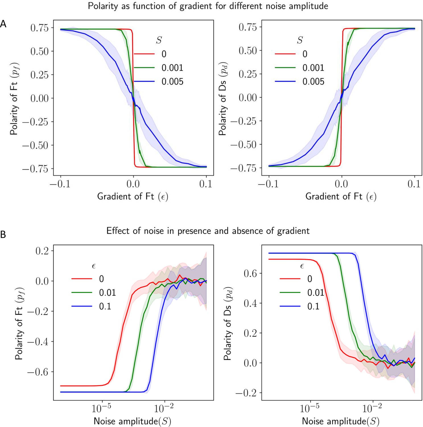
Effect of static spatial noise on the polarization in the presence of gradient cue.

(A) Polarization of Ft ( $p_{f}$ ) and Ds ( $p_{d}$ ) as a function of gradient ( $ϵ$ ) with noise. (B) Polarization of Ft ( $p_{f}$ ) and Ds ( $p_{d}$ ) as a function of noise amplitude ( $S$ ) in the presence of expression gradient. In each panel, the solid lines and the shaded regions mark the average and standard deviations in the polarity over 50 simulations.

Figure 8

Download asset Open asset

Deletion induces a polarity that decays exponentially.

(A) Ft polarization ( $p_{f}$ ) of each cell as a function of distance from the deletion boundary. (B) Decay length of polarization as a function of total protein concentration. (C) Polarization at different locations in the tissue relative to the deletion boundary.

Figure 9 with 1 supplement

Download asset Open asset

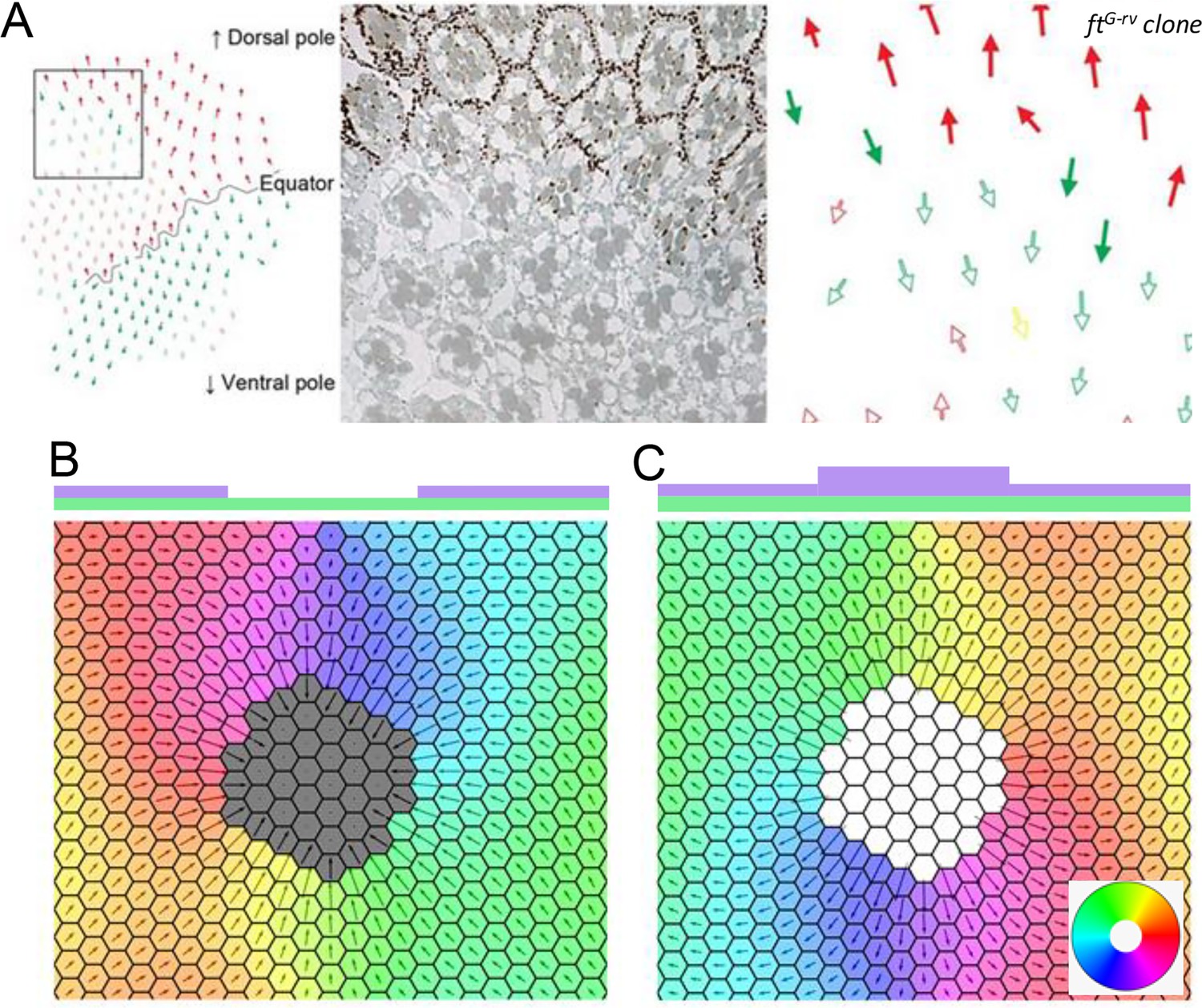
Deletion and upregulation in a 2D layer of tissue.

(A) Experimental images showing a reversal in polarity in Drosophila ommatidia in ft mutant clones (reproduced from Figure 2A of Sharma and McNeill, 2013). (B) Polarization when Ft is removed from a region of the tissue. (C) Polarization when Ft is up-regulated in a region of the tissue. The polygon colors in B and C denote the direction of polarization in each cell. Time evolution of polarization when one of the genes is deleted or upregulated from the circular region at the center of the tissue. The system gets polarized radially from the deletion region.

© 2013, The Company of Biologists Ltd. Panel A was reprinted from Figure 2 A of Sharma and McNeill, 2013, with permission from The Company of Biologists Ltd.; permission conveyed through Copyright Clearance Center, Inc. It is not covered by the CC-BY 4.0 license and further reproduction of this panel would need permission from the copyright holder.

Figure 9—video 1

Download asset

posterframe for video — Time evolution of polarization when one of the genes is deleted or upregulated from the circular region at the center of the tissue.

The system gets polarised radially from the deletion region.

Figure 10 with 1 supplement

Download asset Open asset

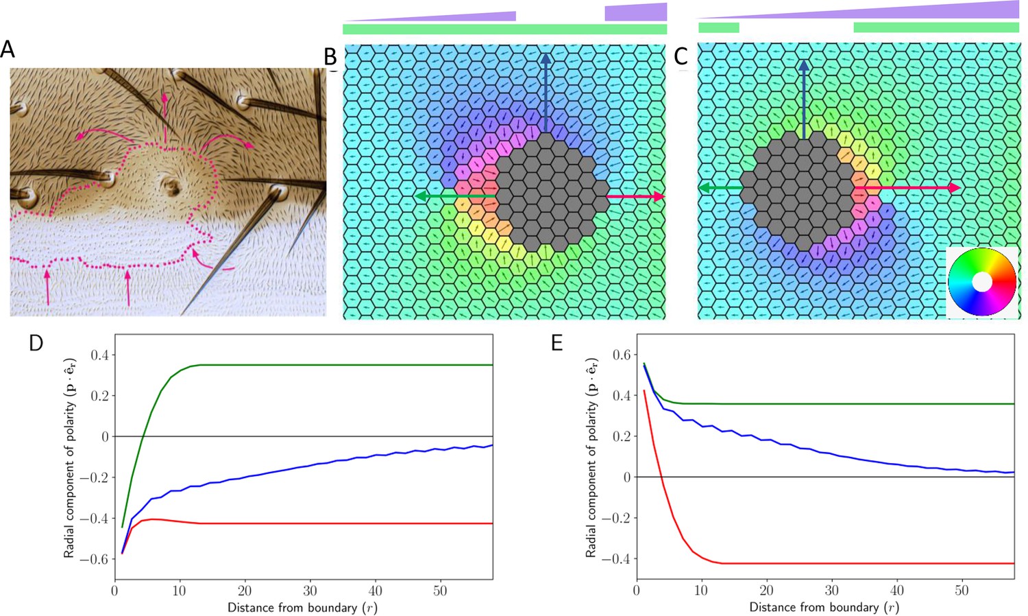
Deletion and gradient can explain domineering non-autonomy.

(A) Experimental image showing the effect of localized perturbation in pre-hairs on Drosophila wing (reproduced from Figure 6A of Chorro et al., 2022). (B) Cell polarization in the tissue in the presence of Ft gradient and its localized loss. (C) Cell polarization in the tissue when Ds has been removed locally while Ft is expressed in a gradient manner. The colors in B and C denote the direction of cell polarization. (D and E) Polarity in the radial direction as a function of distance from the deletion boundary. The color of the trajectory corresponds to the direction in which the arrows point in B (D) and C (E). Time evolution of polarization when one of the proteins is deleted from the central region of the tissue along with a gradient of Ft throughout the tissue.

Figure 10—video 1

Download asset

posterframe for video — Time evolution of polarization when one of the proteins is deleted from the central region of the tissue along with a gradient of Ft throughout the tissue.

The system now evolves with the combined effect of the gradient and the deletion. The cells near the deletion boundary are polarised depending on their distance from deletion boundary.

Additional files

MDAR checklist: https://cdn.elifesciences.org/articles/84053/elife-84053-mdarchecklist1-v2.docx
Download elife-84053-mdarchecklist1-v2.docx

Download links

A two-part list of links to download the article, or parts of the article, in various formats.

Downloads (link to download the article as PDF)

Open citations (links to open the citations from this article in various online reference manager services)

Mendeley

Cite this article (links to download the citations from this article in formats compatible with various reference manager tools)

Divyoj Singh
Sriram Ramaswamy
Mohit Kumar Jolly
Mohd Suhail Rizvi

(2024)

Emergence of planar cell polarity from the interplay of local interactions and global gradients

eLife 13:e84053.

https://doi.org/10.7554/eLife.84053

Sign up for email alerts

Privacy notice