Research Article

Diversity and evolution of cerebellar folding in mammals

Institut Pasteur, Université Paris Cité, Unité de Neuroanatomie Appliquée et Théorique, France
Centre for Health and Cognition, Bath Spa University, United Kingdom
Otto Hahn Group Cognitive Neurogenetics, Max Planck Institute for Human Cognitive and Brain Sciences, Germany
Institute of Neuroscience and Medicine, Brain & Behaviour (INM-7), Research Centre Jülich, FZ Jülich, Germany
Institute of Systems Neuroscience, Medical Faculty, Heinrich Heine University Düsseldorf, Germany
Université Lyon, Université Claude Bernard Lyon 1, CNRS, ENTPE, UMR 5023 LEHNA, France

Sep 22, 2023

https://doi.org/10.7554/eLife.85907

Open access
Copyright information

Figures
Tables
Additional files

12 figures, 3 tables and 4 additional files

Figures

Figure 1

Download asset Open asset

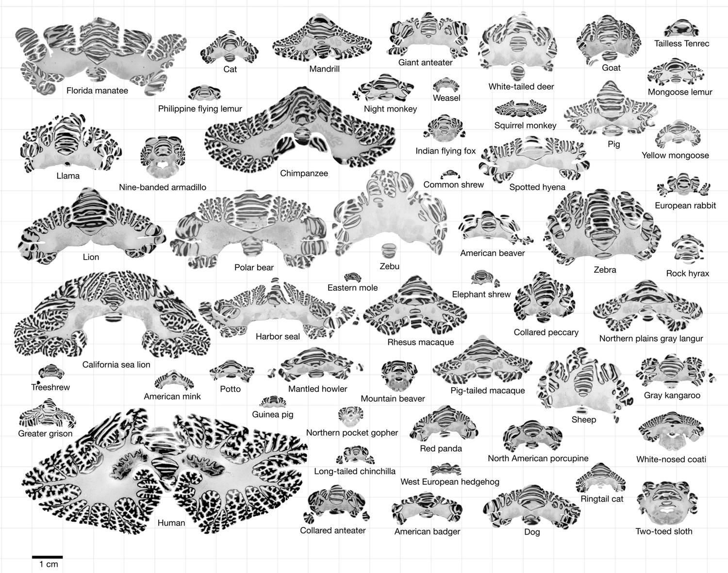
Data.

All coronal cerebellar mid-sections for the different species analysed, at the same scale. This dataset is available online for interactive visualisation and annotation: https://microdraw.pasteur.fr/project/brainmuseum-cb. Image available at https://doi.org/10.5281/zenodo.8020178.

Figure 2

Download asset Open asset

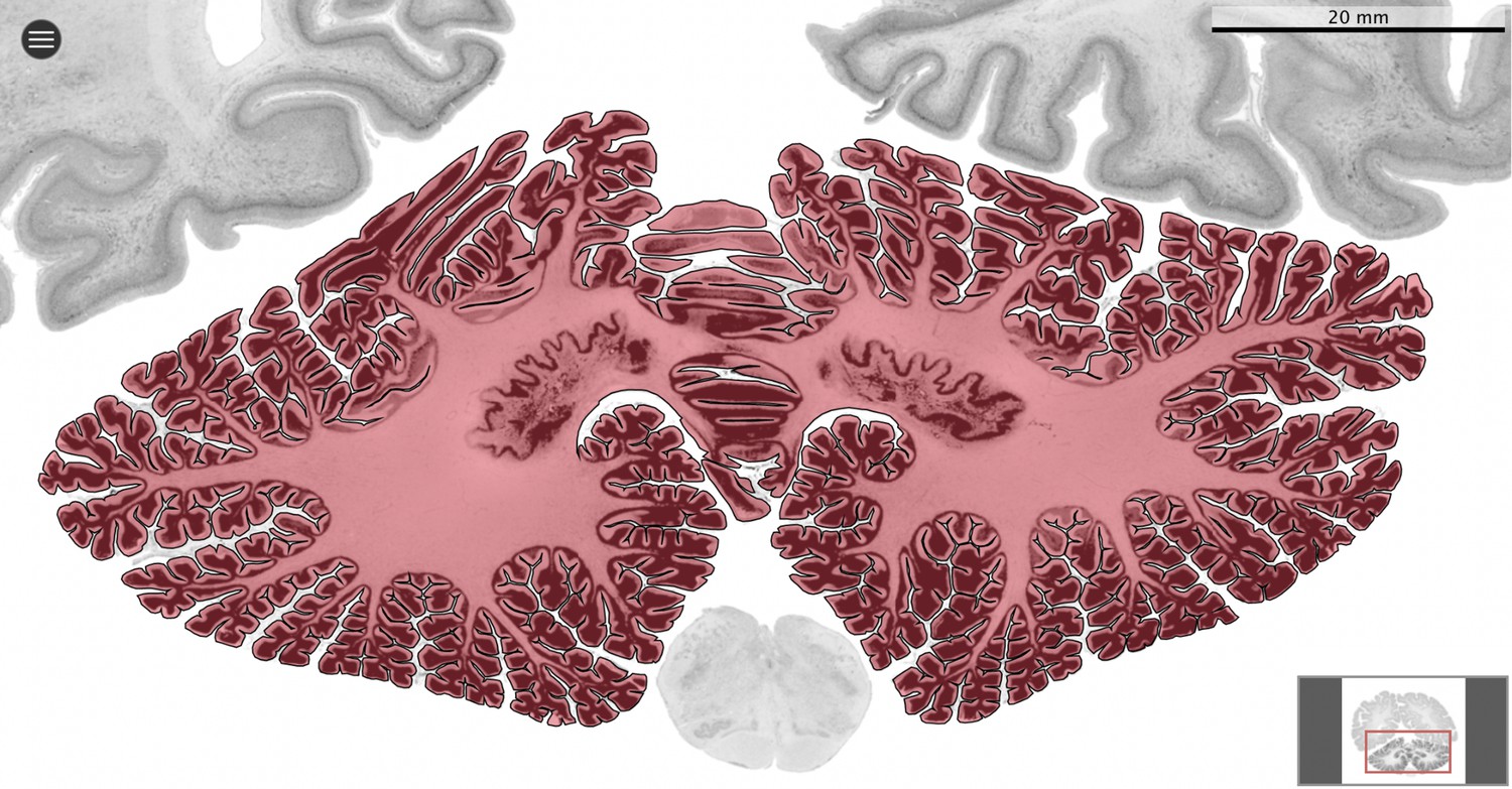
Segmentation.

All datasets were indexed in our collaborative Web application MicroDraw (https://microdraw.pasteur.fr) to interactively view and annotate the sections. The contour of the cerebellum was drawn manually using MicroDraw (black contour). The example image shows the human cerebellum from the BigBrain 20 µm dataset (Amunts et al., 2013).

Figure 3

Download asset Open asset

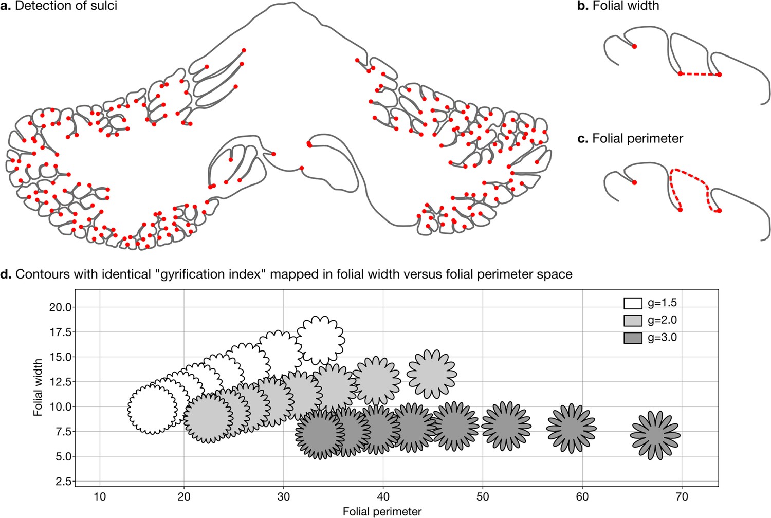
Detection of sulci and measurement of folial width and perimeter.

Sulci were automatically detected using mean curvature filtered at different scales (a). From this, we computed folial width (b) and folial perimeter (c). (d) Folial width and perimeter allow to distinguish folding patterns with the same gyrification index. The three rows of contours have the same gyrification index (top g=1.5, middle g=2.0, bottom g=3.0), however, the gyrification index does not allow distinguishing between contours with many shallow folds and those with few deep ones.

Figure 4

Download asset Open asset

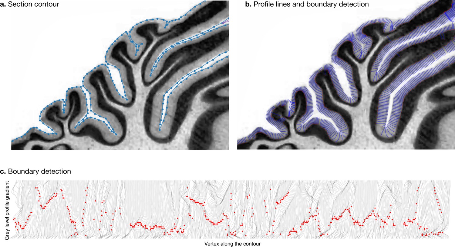
Measurement of molecular layer thickness.

The thickness of the molecular layer was measured automatically from the surface segmentation. (a) Zoom into a manually annotated surface contour. (b) Automatically computed profile lines. (c) Grey level profile gradients and border detection for the whole slice. Red dots indicate detected borders (maximum gradient).

Figure 5

Download asset Open asset

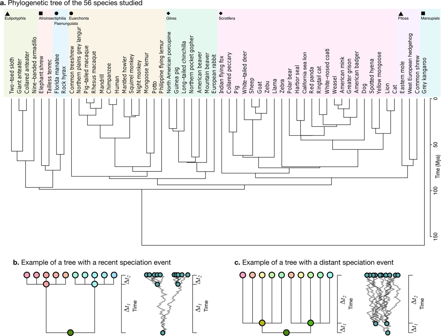
Phylogenetic tree.

(a) The phylogenetic tree for 56 species used in our study was downloaded from the TimeTree website (http://www.timetree.org, Kumar et al., 2017) and coloured in eight groups based on hierarchical clustering of the tree. (b) Not accounting for phylogenetic information can lead to misinterpretations of cross-species relationships. Consider the case of eight species descending from two recent ancestors as in the tree ( $Δ t_{2} ≪ Δ t_{1}$ , adapted from Felsenstein, 1985). Even if their phenotypes evolved randomly (Brownian motion [BM] process in the phenogram to the right), they will seem to be more similar within each group. (c) If the time of split from their common ancestor were more distant ( $Δ t_{2} ≫ Δ t_{1}$ ), this difference would not exist. Real phylogenetic trees embed a complex hierarchical structure of such relationships.

Figure 6 with 1 supplement

Download asset Open asset

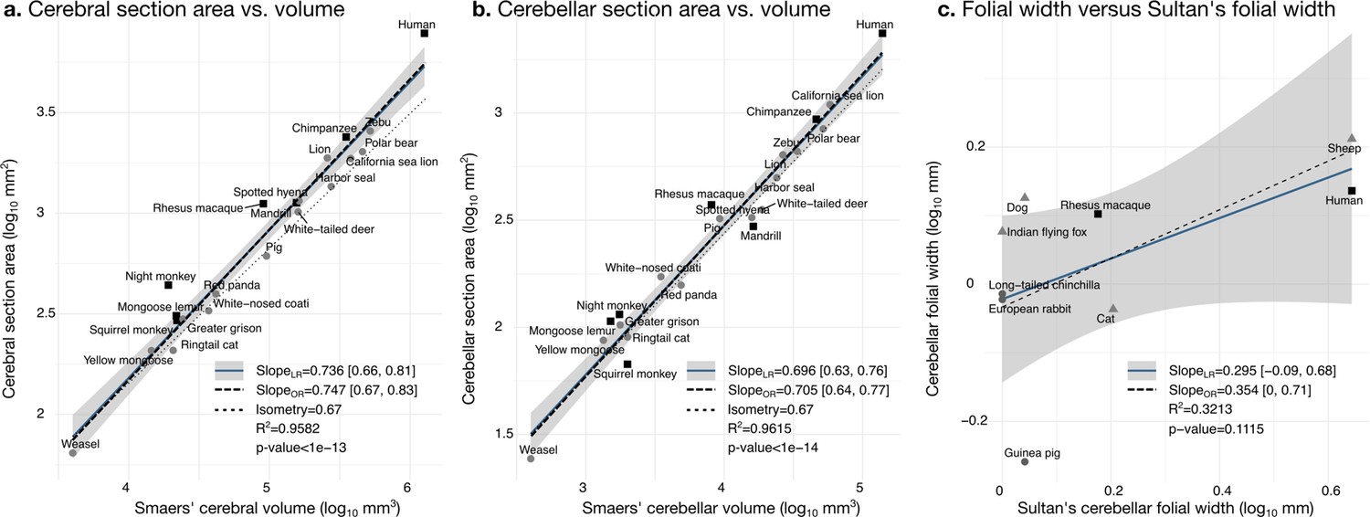
Validation of neuroanatomical measurements.

Comparison of our cortical section area measurement (a) and cerebellar section area (b) with volume measurements from Smaers et al., 2018. (c) Comparison of our folial width measurement with folial width from Sultan and Braitenberg, 1993. The folial width measurement reported by Sultan and Braitenberg, which may include several folia, do not correlate significantly with our measurements (two-tailed p=0.112). LR: linear regression with 95% confidence interval in grey. OR: orthogonal regression.

Figure 6—figure supplement 1

Download asset Open asset

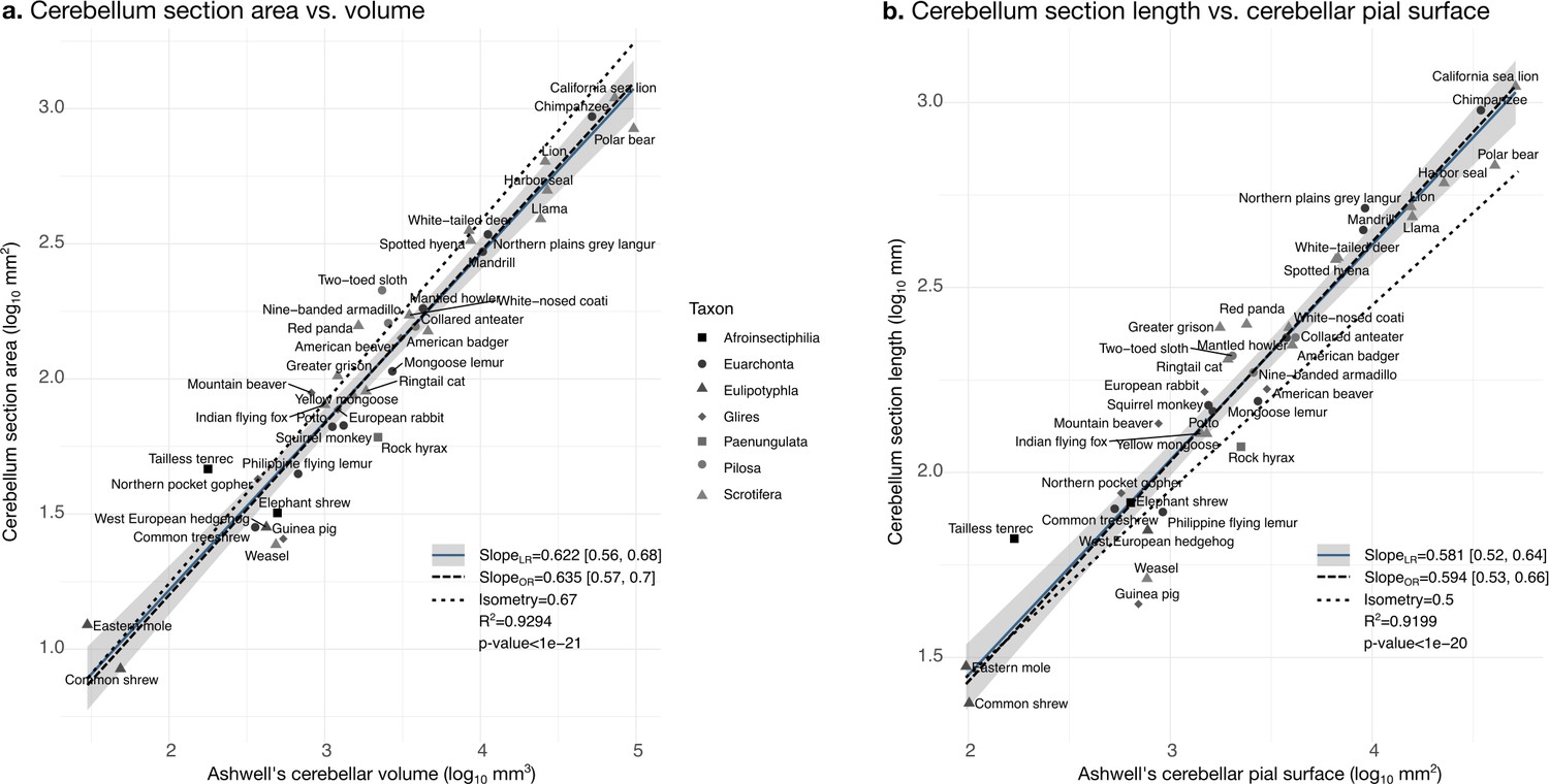
Validation of neuroanatomical measurements: correlation with measurements in Ashwell, 2020.

Comparison of our cerebellar section area measurement (a) and cerebellar section length (b) with cerebellar volume and surface measurements from Ashwell, 2020. Measurements correlate significantly (two-tailed p<1e-20). LR: linear regression with 95% confidence interval in grey. OR: orthogonal regression.

Figure 7

Download asset Open asset

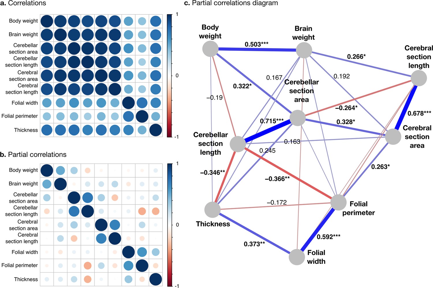
Correlation structure.

(a) Correlation matrix among all phenotypes (all values log₁₀ transformed). (b) Partial correlation matrix. (c) Graph representation of the strongest positive (red) and negative (blue) partial correlations. All correlations are conditional to phylogenetic tree data. Partial correlation significance is indicated by asterisks, *** for p<0.001, ** for p<0.01, * for p<0.05. Partial correlations without asterisks are not significant.

Figure 8

Download asset Open asset

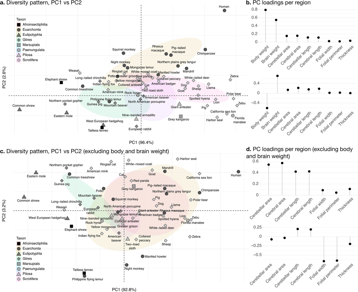
Phylogenetic principal component analysis.

Primates, and especially humans, show particularly large brains given their body size. (a) Pattern of neuroanatomical diversity (PC1 vs. PC2), including body and brain weight. (b) Loadings of the PC1 and PC2 axes displayed in panel a. (c) Pattern of neuroanatomical diversity (PC1 vs. PC2), excluding body and brain weight. (d) Loadings of the PC1 and PC2 axes displayed in panel c.

Figure 9

Download asset Open asset

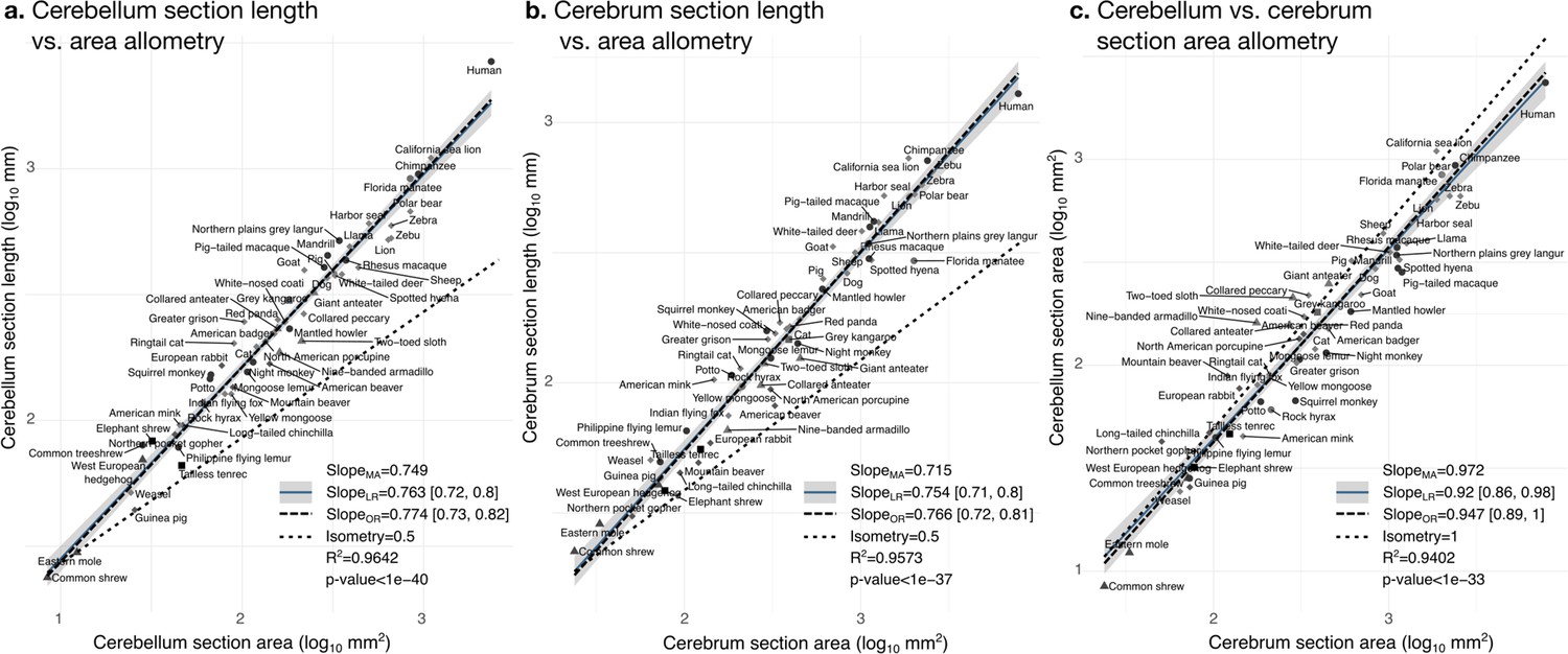
Cerebellum and cerebrum folding and allometry.

The cerebellar and cerebral cortices are disproportionately larger than their volumes, as shown by their hyper-allometry. The cerebellum is slightly but statistically significantly hypo-allometric compared to the cerebrum. (a) Allometry of cerebellum section length vs. cerebellum section area. (b) Allometry of cerebrum length vs. cerebrum section area. (c) Allometry of cerebellum section area vs. cerebrum section area. MA: multivariate allometry. LR: linear regression with 95% confidence interval in grey. OR: orthogonal regression.

Figure 10

Download asset Open asset

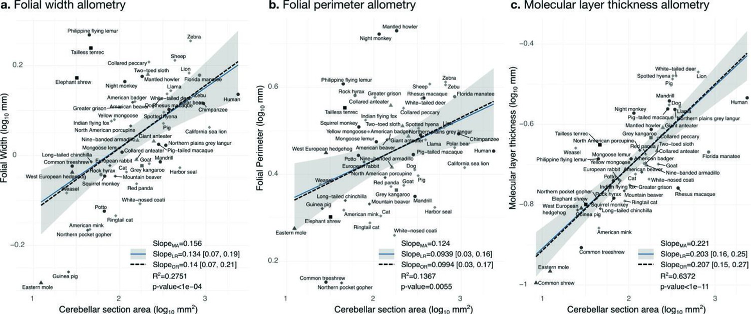
Allometry of folial width, perimeter, and molecular layer thickness.

The geometry of cerebellar folia and molecular layer thickness were largely conserved when compared with changes in total cerebellar size, as revealed by the small allometric slopes. (a) Allometry of folial width vs. cerebellar section area (two-tailed p<1e-5). (b) Allometry of folial perimeter vs. cerebellar section area (two-tailed p=0.005). (c) Allometry of the thickness of the molecular layer vs. cerebellar section area (two-tailed p<1e-12). MA: multivariate allometry. LR: linear regression with 95% confidence interval in grey. OR: orthogonal regression.

Figure 11

Download asset Open asset

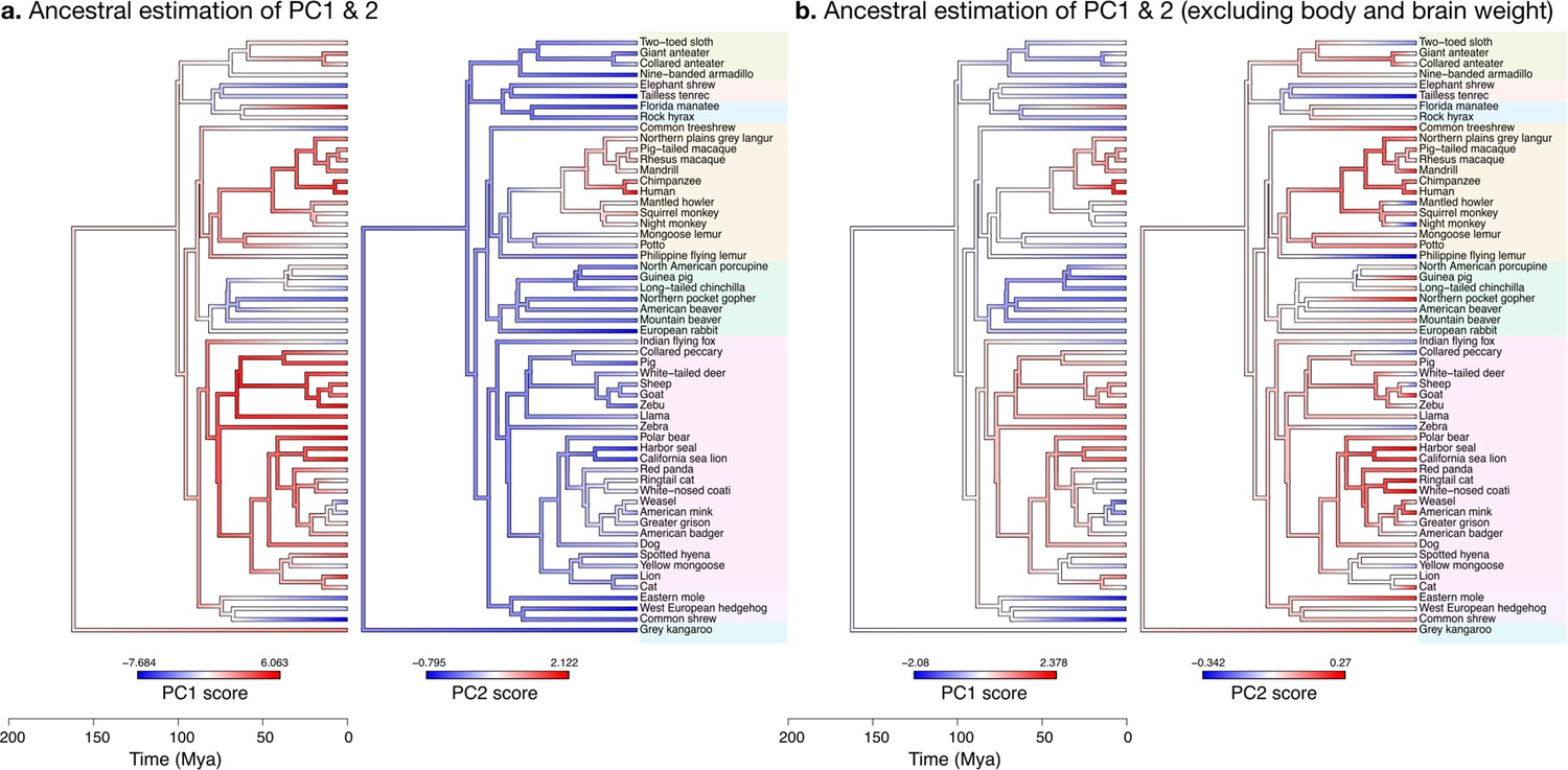
Estimation of ancestral neuroanatomical diversity patterns.

Our analyses show a concerted change in body and brain size, and specific increase in cerebral and cerebellar volume in primates concomitant with an increased number of smaller folia. (a) Ancestral estimation of PC1 and PC2 for neuroanatomical variables plus brain volume. PC1 captures 96.4% of the variance, PC2 captures 2.4%. (b) Ancestral estimation of PC1 and PC2 for neuroanatomical variables, without brain volume. PC1 captures 91.4% of phenotypic variance, PC2 captures 3.6%.

Author response image 1

Download asset Open asset

Statistical power for partial correlation analysis.

(a) Power to detect the observed effect size was computed using 1000 simulations. At each run a sample size varying from 20 to 100 species was generated with 9 variables using the observed variance-covariance matrix. We estimated our power to detect large, medium and small partial correlations. The simulations show that with N=56 species we had excellent power to detect large and medium partial correlations, and close to 80% power to detect small partial correlations. (b) Power would decrease if the allometry in our data were not as strong as it is, which makes our 9 variables strongly correlated instead of independent. For illustration, we modified the observed variance-covariance matrix to weaken its allometry: we took the square root of all eigenvalues, and scaled the resulting variance-covariance matrix so that its determinant would be the same as in the observed matrix. This results in a less anisotropic, more “spherical” variance-covariance matrix. As expected, statistical power decreases (however, it is still ~90% for large partial correlations). Code for the simulations was uploaded to the accompanying GitHub repository.

Tables

Table 1

Definition of the variables used in the current study and their sources.

Variable name	Definition	Source
Cerebellar section area	Area of the cerebellar mid-section (mm²)	Measured
Cerebellar section length	Perimeter around the cerebellar pial surface of mid-section (mm)	Measured
Folial width (cerebellum)	Euclidean distance between the two flanking sulci of a folium, averaged for all folia in the mid-section (mm; Figure 3b)	Measured
Folial perimeter (cerebellum)	Perimeter along the cerebellar pial surface between the two flanking sulci of a folium, averaged for all folia in the mid section (mm; Figure 3c)	Measured
Thickness (cerebellum)	Thickness of the molecular layer for the cerebellar mid section, averaged from the lengths profile lines that bisect the molecular layer from its border with the pial surface to its border with the granular surface (mm; Figure 4)	Measured
Cerebral section area	Area of the cerebral mid-section (mm²)	Measured
Cerebral section length	Perimeter around the cerebral pial surface of mid-section (mm)	Measured
Brain weight	Weight of the whole brain, including cerebrum and cerebellum (g)	Ballarin et al., 2016; Burger et al., 2019; Smaers et al., 2021
Body weight	Weight of the whole body (g)	Ballarin et al., 2016; Burger et al., 2019; Smaers et al., 2021
Cerebellar volume	Volume of the entire cerebellum, estimated from 2D histological sections or MRI (mm³)	Smaers et al., 2018
Cerebral volume	Volume of the entire cerebrum, estimated from 2D histological sections or MRI (mm³)	Smaers et al., 2018
Sultan’s folial width	Length of a cerebellar fold in a cross-section orthogonal to the fold axis: each fold may contain several individual folia	Sultan and Braitenberg, 1993

Table 2

Ranking of phylogenetic comparative models.

Results based on the Akaike information criterion corrected for small sample sizes (AICc). The best fit to the data (smallest AICc value) was obtained for the Ornstein-Uhlenbeck model.

Ranking	Model	AICc	Log-likelihood
1	Ornstein-Uhlenbeck (OU)	−360.64	252.48
2	Early burst (EB)	−254.03	188.89
3	Brownian motion (BM)	−227.73	174.62

Table 3

Multivariate allometry pattern.

The pattern is represented by the loadings of each measurement in the first principal component (PC1, same as Figure 8b). Allometric slopes for each pair of variables can be obtained by dividing their loadings. For example, the slope for the cerebellum section length versus cerebellum section area reported in Figure 9a is 0.1138/0.1519 ~ 0.749.