Multisensory integration operates on correlated input from unimodal transient channels
Figures
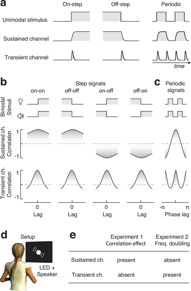
Sustained vs. transient channels.
(a) Responses of sustained and transient channels to onset and offset step stimuli, and periodic signals comprising sequences of onsets and offsets. Note that while the sustained channels closely follow the intensity profile of the input stimuli, transient channels only respond to changes in stimulus intensity, and such a response is always positive, irrespective of whether stimulus intensity increases or decreases. Therefore, when presented with periodic signals, while the sustained channels respond at the same frequency as the input stimulus (frequency following), transient channels respond at a frequency that is twice that of the input (frequency doubling). (b) Synchrony as measured from cross-correlation between pairs of step stimuli, as seen through sustained (top) and transient (bottom) channels (transient and sustained channels are simulated using Equations 1; 10, respectively). Note how synchrony (i.e., correlation) for sustained channels peaks at zero lag when the intensity of the input stimuli changes in the same direction, whereas it is minimal at zero lag when the steps have opposite polarities (negatively correlated stimuli). Conversely, being insensitive to the polarity of intensity changes, synchrony for transient channels always peaks at zero lag. (c) Synchrony (i.e., cross-correlation) of periodic onsets and offset stimuli as seen from sustained and transient channels. While synchrony peaks once (at zero phase shift) for sustained channels, it peaks twice for transient channels (at zero and pi radians phase shift), as a consequence of its frequency-doubling response characteristic. (d) Experimental apparatus: participants sat in front of a black cardboard panel with a circular opening, through which audiovisual stimuli were delivered by a white LED and a loudspeaker. (e) Predicted effects of experiments 1 and 2 depending on whether audiovisual integration relies on transient or sustained input channels. The presence of the effects of interest in both experiments or the lack thereof indicates an inconclusive result, not interpretable in the light of our hypotheses.
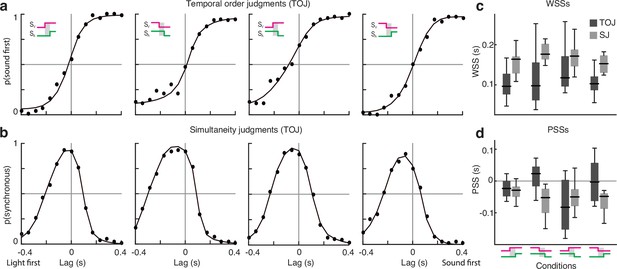
Experiment 1: results.
(a) Responses in the temporal order judgment (TOJ) task and psychometric fits (averaged across participants) for the four experimental conditions. (b) Responses in the simultaneity judgment (SJ) task and psychometric fits (averaged across participants) for the four experimental conditions. Each dot in (a, b) corresponds to 80 trials. (c) Window of subjective simultaneity for each condition and task. (d) Point of subjective simultaneity for each condition and task.
-
Figure 2—source data 1
Data of the temporal order judgment (TOJ) task.
- https://cdn.elifesciences.org/articles/90841/elife-90841-fig2-data1-v1.zip
-
Figure 2—source data 2
Data of the simultaneity judgment (SJ) task.
- https://cdn.elifesciences.org/articles/90841/elife-90841-fig2-data2-v1.zip
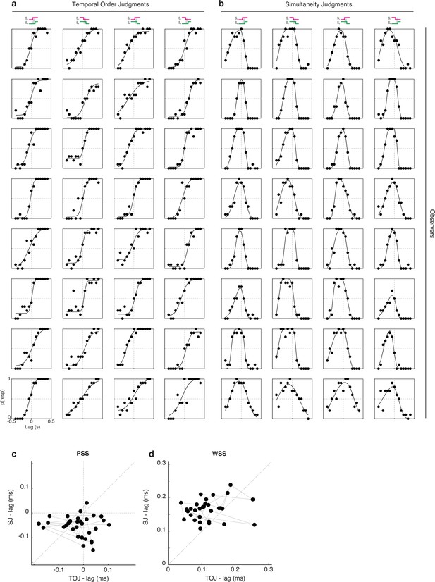
Results and psychometric fits of experiment 1.
Data from different observers are represented in different rows. (a) represents the data of the temporal order judgment (TOJ) task. (b) represents the data of the simultaneity judgment (SJ) task. The icons on top represent the different conditions. Each dot corresponds to 10 trials. (c) represents the scatterplot of the point of subjective simultaneity (PSS) measured with the TOJ plotted against the PSS measured with the SJ. (d) represents the scatterplot of the window of subjective simultaneity (WSS) measured with the TOJ plotted against the PSS measured with the SJ. Each dot in (c, d) represents the PSS or WSS from one condition and observer (i.e., there are four dots for each observer, one per condition); datapoints from the same participant are linked by a gray line.
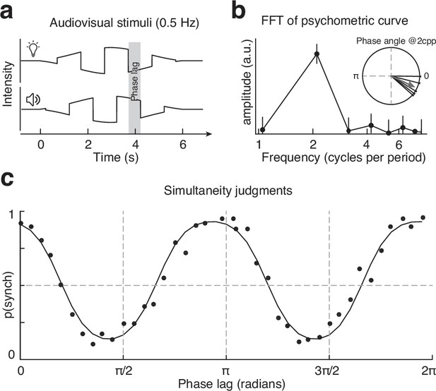
Experiment 2: stimuli and results.
(a) Schematic representation of the periodic stimuli. (b) Frequency domain representation of the psychometric function: note the amplitude peak at two cycles per period. Errorbars represent the 99% CIs. The inset represents the phase angle of the two cycles per period frequency component for each participant (thin lines) and the average phase (arrow). (c) Results of experiment 2 and psychometric fit, averaged across all participants. Each dot corresponds to 75 trials.
-
Figure 3—source data 1
Data of the simultaneity judgment (SJ) task.
- https://cdn.elifesciences.org/articles/90841/elife-90841-fig3-data1-v1.zip
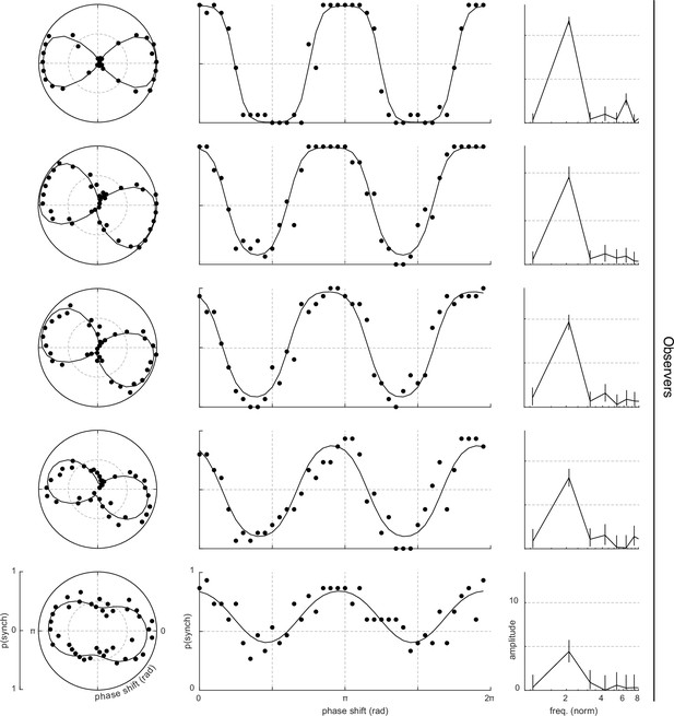
Results and psychometric fits of experiment 2.
Data from different observers are represented in different rows. The first four columns represent the data in polar coordinates, whereas the second column represent the same dataset in Cartesian coordinates. The counter-clockwise rotation of the polar psychometric functions indicates that maximum perceived synchrony across the senses occurs when vision changes slightly before audition. Each dot corresponds to 15 trials. The last column represents the psychometric curve in the frequency domain: note the peak at 2 cpp in every participant, indicating the frequency-doubling effect. The errorbars in the last column represent the 99% CIs.
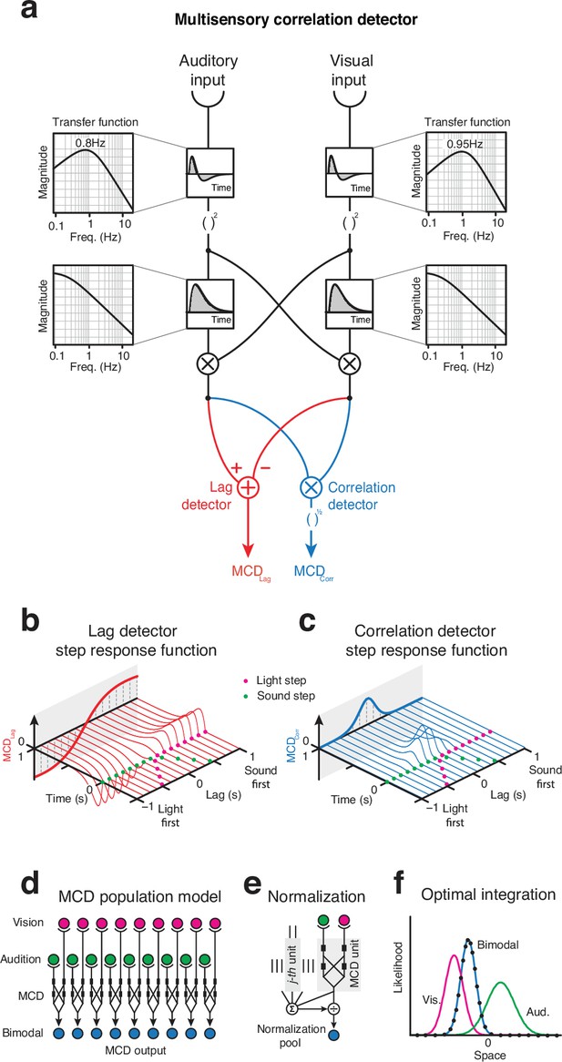
Multisensory correlation detector (MCD) model.
(a) Model schematics: the impulse-response functions of the channels are represented in the small boxes, and call-outs represent the transfer functions. (b) Lag detector step responses as a function of the lag between visual and acoustic steps. (c) Correlation detector responses as a function of the lag between visual and acoustic steps. (d) Population of MCD units, each receiving input from spatiotopic receptive fields. (e) Normalization, where the output of each unit is divided by the sum of the activity of all units. (f) Optimal integration of audiovisual spatial cues, as achieved using a population of MCDs with divisive normalization. Lines represent the likelihood functions for the unimodal and bimodal stimuli; dots represent the response of the MCD model, which is indistinguishable from the bimodal likelihood function.

Multisensory correlation detector (MCD) simulations of experiments 1 and 2.
(a) Schematics of the observer model, which receives input from one MCD unit to generate a behavioral response. The output of the MCD unit is integrated over a given temporal window (whose width depends on the duration of the stimuli) and corrupted by late additive noise before being compared to an internal criterion to generate a binary response. Such a perceptual decision-making process is modeled using a generalized linear model (GLM), depending on the task, the predictors of the GLM were either (Equation 8) or (Equation 9). (b) Responses for the temporal order judgment (TOJ) task of experiment 1 (dots) and model responses (red curves). (c) Responses for the simultaneity judgment (SJ) task of experiment 1 (dots) and model responses (blue curves). (d) Experiment 2 human (dots) and model responses (blue curve). (e) Scatterplot of human vs. model responses for both experiments.
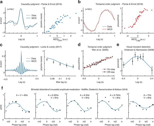
Multisensory correlation detector (MCD) simulations of published results.
(a) Results of the causality judgment task of Parise and Ernst, 2016. The left panel represents the empirical classification image (gray) and the one obtained using the MCD model (blue). The right panel represents the output of the model plotted against human responses. Each dot corresponds to 315 responses. (b) Results of the temporal order judgment task of Parise and Ernst, 2016. The left panel represents the empirical classification image (gray) and the one obtained using the MCD model (red). The right panel represents the output of the model plotted against human responses. Each dot corresponds to 315 responses. (c) Results of the causality judgment task of Locke and Landy, 2017. The left panel represents the empirical classification image (gray) and the one obtained using the MCD model (blue). The right panel represents the effect of maximum audiovisual lag on perceived causality. Each dot represents on average 876 trials (range = [540, 1103]). (d) Results of the temporal order judgment task of Wen et al., 2020. Squares represent the onset condition, whereas circles represent the offset condition. Each dot represents ≈745 trials. (e) Results of the detection task of Andersen and Mamassian, 2008, showing auditory facilitation of visual detection task. Each dot corresponds to 336 responses. (f) Results of the audiovisual amplitude modulation detection task of Nidiffer et al., 2018, where the audiovisual correlation was manipulated by varying the frequency and phase of the modulation signals. Each dot represents ≈140 trials. The datapoint represented by a star corresponds to the stimuli displayed in Figure 6—figure supplement 5.
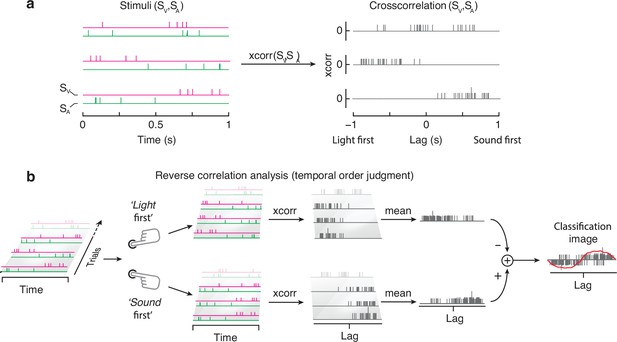
Stimuli and reverse correlation analyses of Parise and Ernst, 2016.
(a) represents three pairs of audiovisual stimuli (left) and their cross-correlation (right). (b) shows a schematic representation of the reverse correlation analyses. Adapted from Figure 2 of Parise and Ernst, 2016.

Stimuli of Locke and Landy, 2017.
Three example pairs of audiovisual stimuli, and their cross-correlogram. Note how the stimuli vary in both terms of temporal rate (i.e., total number of clicks and flashes) and audiovisual correlation (with the bottom one being fully correlated).
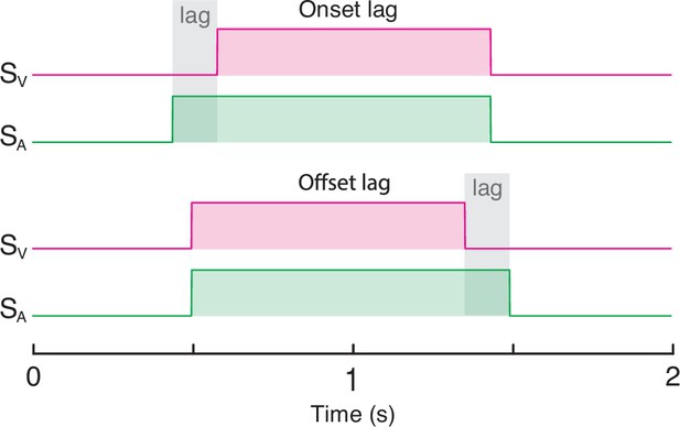
Stimuli of Wen et al., 2020.
Stimuli consisted of rectangular temporal envelopes, with a variable audiovisual lag either at the onset (top) or offset (bottom). The amount of audiovisual lag varied across trials, following a staircase procedure.

Stimuli of Andersen and Mamassian, 2008.
Stimuli consisted of on-steps, with a parametrical manipulation of the lag between vision and audition, determined using the method of constant stimuli.
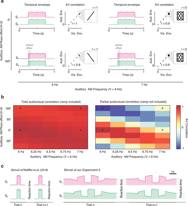
Stimuli of Nidiffer et al., 2018.
Stimuli consisted of a sinusoidal amplitude modulation over a pedestal intensity (a). The pedestal had a 10 ms linear ramp at onset and offset. While the visual sinusoidal amplitude modulation was constant throughout the experiment (frequency = 6 Hz, zero phase offset), the auditory amplitude modulation varied in both frequency (from 6 Hz to 7 Hz, in five steps) and phase offset (from 0 to 360°, in eight steps). Next to each pair of stimuli, we represent the scatterplot of the visual and auditory envelopes, which highlight the audiovisual correlation. The call-out boxes zoom in on the correlation between the audiovisual sinusoidal amplitude modulation (excluding the linear onset and offset ramps), whereas the main scatterplots also display the ramps. (b) represents the audiovisual Pearson correlation for all the stimuli used by Nidiffer et al. The left panel shows the total audiovisual correlation, which was calculated while also including the onset and offset ramps; the right panel represents the partial correlation, calculated by only considering the sinusoidal amplitude modulation (i.e., the area inside the call-outs in a) without considering the onset and offset linear ramps as done in Nidiffer et al., 2018. Note that once the ramps are included in the analyses, all audiovisual stimuli are strongly correlated (with only minor differences across conditions). The stars in the correlation matrices mark the cells corresponding to the four stimuli represented in (a), and the datapoints represented by a star in Figure 5f. (c) displays a comparison between the stimuli used by Nidiffer et al., 2018 and our experiment 2. Both the time axis (abscissa) and the intensity envelope (ordinate) are here drawn to scale. Although both experiments consist of stimuli with periodic amplitude modulations, there are key important differences. First off, while between two consecutive trials the visual and auditory stimuli were completely off in Nidiffer, in our study the pedestal was always present (without any interruptions across consecutive trials). That introduces transients in Nidiffer’s study both at the beginning and the end of each stimulus, which are absent in our stimuli. The relative magnitude of such transients to the comparatively low depth of amplitude modulation (of the sinusoidal component) is the ultimate reason for the absence of frequency doubling in Nidiffer et al., 2018. In our study, transients at the beginning and end of each trial are prevented by playing a constant pedestal stimulus level across trials, and by applying a Gaussian envelope to the depth of our square-wave modulation. Additionally, it is important to stress the obvious difference in the duration and frequency of the stimuli used in the two studies. Specifically, our stimuli were 12 times longer than the stimuli of Nidiffer, but the frequency of amplitude modulation of our study was about 12 times lower (varying depending on the various conditions of Nidiffer et al.). Finally, note the difference in the depth of amplitude modulation across the two experiments.
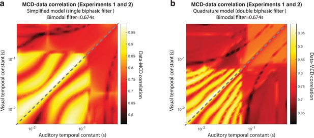
Effect of unimodal temporal constants on the goodness of fit (Pearson correlation) between the multisensory correlation detector (MCD) model and the data from our experiments 1 and 2.
(a) represents the simplified model, with a single biphasic temporal filter. (b) represents the full model, with unimodal temporal filters in quadrature pairs.

Effect of previous trial.
Psychometric surfaces for Experiments 1 and 2 plotted against the lag in the current vs. the previous trial. While psychophysical responses are strongly modulated by the lag in the last trial (horizontal axis), they are relatively unaffected by the lag in the previous trial (vertical axis).
Tables
Sample size of the datasets modeled and analyzed in the present study.
Two of the datasets listed here (i.e., experiment 1 and Parise and Ernst, 2016) consisted of two tasks, each tested on the same pool of observers. The last row represents the total number of observers and trials, the average number of trials per participant, and the average correlation between multisensory correlation detector (MCD) simulations and human data. Note how the revised MCD tightly replicated human responses in all of the datasets included in this study, despite major differences in stimuli, tasks, and sample sizes of the individual studies (see last column).
| Dataset | Task | Number of observers | Number of trials | Trials for observer | MCD-data correlation |
|---|---|---|---|---|---|
| Experiment 1 | Simultaneity judgment | 8 | 4800 | 600 | 0.99 |
| Temporal order judgment | 4800 | 600 | 0.99 | ||
| Experiment 2 | Simultaneity judgment | 5 | 3000 | 600 | 0.98 |
| Parise and Ernst, 2016 | Causality judgment | 5 | 9300 | 1860 | 0.98 |
| Temporal order judgment | 9300 | 1860 | 0.99 | ||
| Locke and Landy, 2017 | Causality judgment | 10 | 7200 | 720 | 0.99 |
| Wen et al., 2020 | Temporal order judgment | 57 | 22,337 | ≈392 | 0.97 |
| Andersen and Mamassian, 2008 | Transient detection | 13 | 2352 | ≈181 | 0.91 |
| Nidiffer et al., 2018 | Modulation detection | 12 | 5604 | 467 | 0.89 |
| Overall | 110 | 68,693 | ≈624 | 0.97 |
Results of Friedman test and Bayesian repeated measures ANOVA for experiment 1.
Four separate Friedman tests were used to assess whether the four experimental conditions differed in terms of point of subjective simultaneity (PSS) and window of subjective simultaneity (WSS) in the temporal order judgment (TOJ) and simultaneity judgment (SJ) tasks. The first column represents the variables, the second the value and the degrees of freedom (in brackets), and the third the p-value. Given that we ran four tests on the same dataset, statistical significance should be computed by comparing the p-value against a Bonferroni-adjusted alpha level of 0.0125 (i.e., 0.05/4). The last column represents the Bayes factor BF01 in favor of the null hypothesis as calculated using Bayesian repeated measures ANOVA using the statistical software JASP (JASP Team 2024; version 0.18.3) with the default settings. Together with the Friedman test, the present analyses provide further converging evidence for the lack of meaningful differences across the two tasks and four conditions of experiment 1.
| Friedman test | Bayesian ANOVA | ||
|---|---|---|---|
| (df) | p-Value | BF01 | |
| PSS (TOJ) | 6.15 (3) | 0.1045 | 2.833 |
| PSS (SJ) | 2.85 (3) | 0.4153 | 2.237 |
| WSS (TOJ) | 2.55 (3) | 0.4663 | 2.570 |
| WSS (SJ) | 5.55 (3) | 0.1357 | 1.452 |
Additional files
-
MDAR checklist
- https://cdn.elifesciences.org/articles/90841/elife-90841-mdarchecklist1-v1.docx
-
Source code 1
MATLAB implementations of the MCD model and the quadrature MCD model.
- https://cdn.elifesciences.org/articles/90841/elife-90841-code1-v1.zip


