Figures and data in Heterozygote advantage can explain the extraordinary diversity of immune genes | eLife

Figures
Additional files

10 figures and 1 additional file

Figures

Figure 1

Download asset Open asset

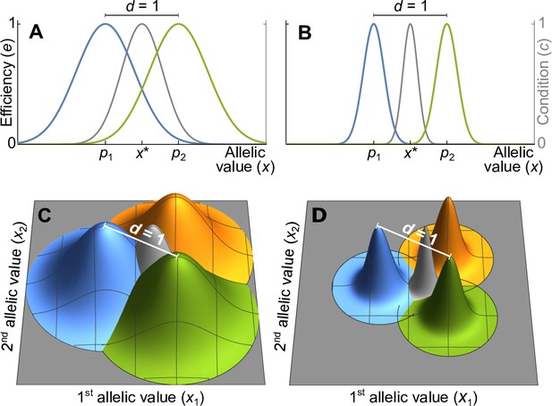
Efficiency against two pathogens (coloured lines in A–B) and three pathogens (coloured cones in C–D) as a function of allelic values $x$ .

Efficiencies are modeled with Gaussian functions with pathogen optima at equal distances $d = 1$ (indicated by $p_{1}$ and $p_{2}$ in A, B). The width of the Gaussian functions, which determine how severely pathogens affect hosts with suboptimal major histocompatibility complex (MHC) molecules, is given by the virulence parameter $v$ . With high virulence ( $v = 7$ , narrow Gaussians in B, D), alleles away from the optima have a low efficiency, while for a low virulence ( $v = 2.5$ , wide Gaussians in A, C) efficiency is higher. Grey lines and cones give the condition $c$ of homozygote individuals. The generalist allele, maximising condition, is located at the centre with equal distance to all pathogen optima (indicated by $x^{*}$ in A, B).

Figure 2

Download asset Open asset

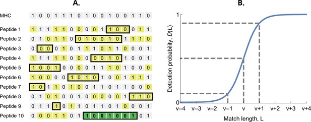
Detection probability in the bit-string model.

(A) Major histocompatibility complex (MHC) bit-string matching against a pathogen with $n_{p e p} = 10$ peptides. Yellow indicates a match between MHC and peptide bits. The longest consecutive match per peptide ( $L$ ) is indicated with a black box. The longest match over all peptides occurs for the last peptide, marked in green, with match length $L = 7$ . (B) Detection probability for peptides as a function of match length $L$ (Equation 2 with $a = \log (9)$ ). The dashed lines indicate, from left to right, 10%, 50%, and 90% detection probability.

Figure 3

Download asset Open asset

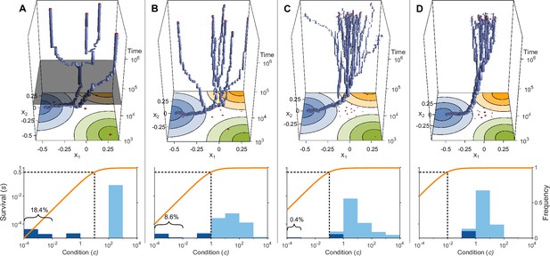
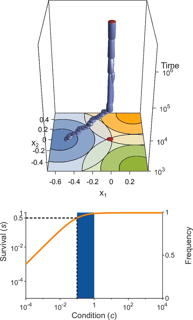
Evolution of allelic values under the Gaussian model in the presence of three pathogens (arranged as in Figure 1D) for four different values of the survival half-saturation constant $K$ (A: $K = 10$ , B: $K = 1$ , C: $K = 0.1$ , D: $K = 0.01$ ; dashed line in lower panel).

The top panel shows individual-based simulations. The two horizontal axes give the two allelic values $x = (x_{1}, x_{2})$ that characterise an allele, while the vertical axis shows evolutionary time. The thickness of the blue tubes is proportional to allele frequencies. Allelic values at the last generation are projected as red dots on the top as well as on the bottom plane. Coloured circles represent the contour lines of the Gaussian efficiency functions $e_{k} (x)$ as shown in Figure 1D. In all simulations, gradual evolution leads towards the generalist allele $x^{*} = (0, 0)$ and branching occurs in its neighbourhood, as predicted by our analytical derivations (Appendix ‘The evolutionarily singular point’). In (A) there are three consecutive branching events with the second branching event marked by the grey plane ( $n_{e} = 4.0$ ; for details regarding $n_{e}$ , see the legend of Figure 4). (B and C) show that, as $K$ decreases, the number of branching events increases, resulting in more coexisting alleles ( $n_{e} = 7.8$ and $n_{e} = 16.5$ , respectively). Finally, (D) reveals that, as $K$ decreases even further such that already low condition values result in high survival, the number of branching events decreases again, resulting in a set of alleles closely clustered around the generalist allele ( $n_{e} = 10.2$ ). The bottom panel shows survival $s$ as a function of condition $c$ as defined by Equation 5 on a log-log scale (orange line, left vertical axis) and the frequencies of individual conditions at the final generation (dark blue bars for homozygotes and light blue bars for heterozygotes, right vertical axis; conditions from 0 to $10^{- 4}$ are incorporated into the first bar). These panels show that increased allelic diversity results in a lower proportion of homozygote individuals, which have lower survival. Other parameter values: $v = 7$ , $N = 2 \times 10^{5}$ , $μ = 10^{- 6}$ , and $δ = 0.016$ .

Figure 4

Download asset Open asset

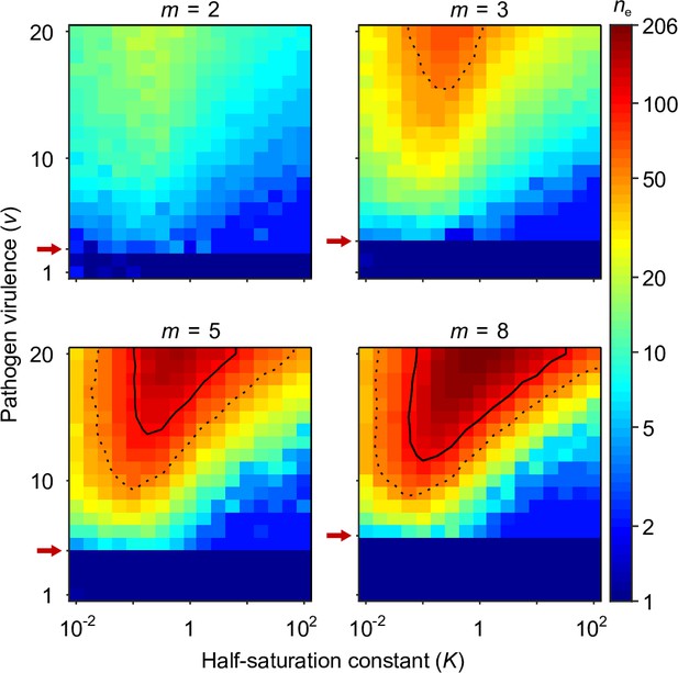
Number of coexisting alleles under the Gaussian model for $m$ pathogens as a function of pathogen virulence $v$ and the survival half-saturation constant $K$ .

Figures are based on a single individual-based simulation per pixel and run for 10⁶ generations, assuring that the equilibrium distribution of alleles is reached. Results are reported in terms of the effective number of alleles $n_{e}$ , which is a conservative measure for the number of alleles, discounting for rare alleles present at mutation-drift balance (see Appendix ‘Eﬀective number of alleles’). The clear pattern in the figures indicates a high degree of determinism in the simulations. Using population size $N = 10^{5}$ and per capita mutation probability $μ = 5 \times 10^{- 7}$ , the expected $n_{e}$ under mutation-drift balance alone equals 1.2 (see Appendix ‘Eﬀective number of alleles’). Dashed and solid lines give the contours for $n_{e} = 50$ and $n_{e} = 100$ , respectively. Red arrows indicate $v = 2 \sqrt{m}$ , the threshold for polymorphism to emerge from branching (Equation A46). Accordingly, simulations in the dark blue area result in a single abundant allele with $n_{e}$ close to one. Other parameters: expected mutational step size $δ = 0.03$ .

Figure 5

Download asset Open asset

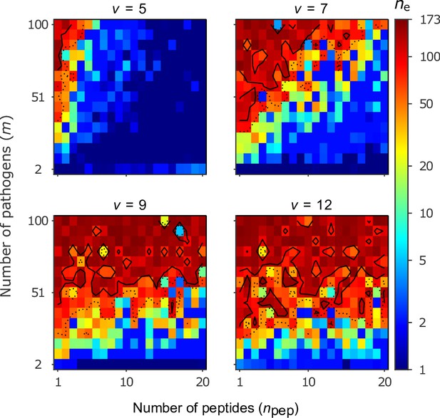
Number of coexisting alleles for the bit-string model for four values of virulence $v$ as a function of the number of pathogens $m$ (increased in steps of 7) and the number of peptides per pathogen $n_{p e p}$ .

Figures are based on a single individual-based simulation per pixel and run for 10⁶ generations. Results are reported in terms of the effective number of alleles $n_{e}$ , which discounts for rare alleles present at mutation-drift balance (see Appendix ‘Eﬀective number of alleles’). Using population size $N = 10^{5}$ and per capita mutation probability $μ = 5 \times 10^{- 6}$ , the expected $n_{e}$ under mutation-drift balance alone equals 3. Dashed and solid lines give the contours for $n_{e} = 50$ and $n_{e} = 100$ , respectively. Evolution started from populations monomorphic for a random allele, and run for $2 \times 10^{6}$ generations, assuring that the equilibrium distribution of alleles is reached. Other parameters: half-saturation constant $K = 1$ .

Figure 6

Download asset Open asset

A simulation run showing the evolution of allelic diversity under the bit-string model in the presence of $m = 12$ pathogens.

(A) shows the number of alleles $n$ and the effective number of alleles $n_{e}$ as a function of time (on a log-log scale). (B–D) give survival $s$ as a function of condition $c$ as defined by Equation 5 on a log-log scale (orange line, left vertical axis) and the distribution of conditions at three time points (B $t = 100$ , C $t = 3900$ , D $t = 10^{6}$ ; vertical green dashed lines in A), with dark blue bars for homozygotes and light blue bars for heterozygotes (right vertical axis; conditions from 0 to $10^{- 4}$ are incorporated into the first bar, and conditions from 10⁴ and greater are incorporated in the last bar). This shows that as allelic diversity increases, the frequency of homozygotes with low survival decreases. The black dashed lines indicate the value of $K = 1$ . Other parameter values: $v = 7$ , $m = 12$ , $n_{p e p} = 3$ , $N = 10^{5}$ , $μ = 5 \times 10^{- 6}$ .

Appendix 2—figure 1

Download asset Open asset

Evolution of allelic values in the presence of three pathogens.

This figure is analogous to Figure 3 (see that legend for details) but with wider Gaussians ( $v = 2.5$ , as in Figure 1C). As a consequence, the condition for evolutionary branching ( $v > 2 \sqrt{m}$ ) is not fulfilled and the evolutionary dynamics result in a monomorphic population consisting essentially of only the generalist allele $x^{*} = (0, 0)$ . This result is independent of the half-saturation constant $K$ , here chosen to be $K = 10$ .

Appendix 4—figure 1

Download asset Open asset

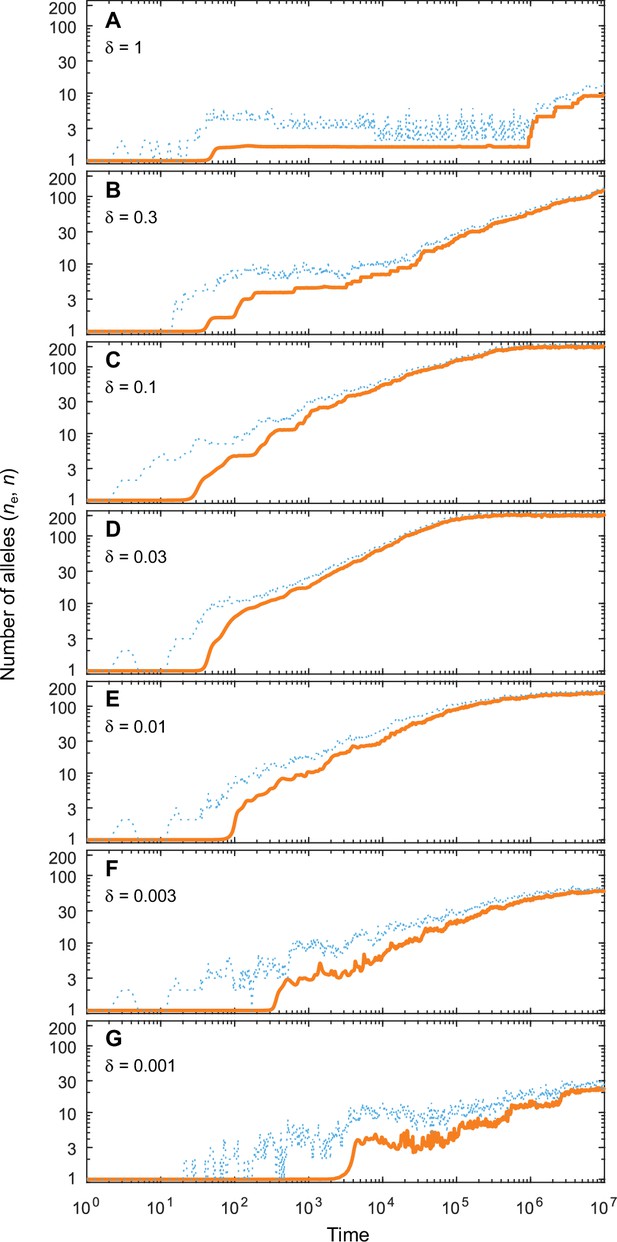
Number of coexisting alleles as they emerge in individual-based simulations for different expected mutational step sizes $δ$ and eight pathogens ( $m = 8$ ).

Parameters are chosen such that up to 200 alleles can evolve ( $K = 0.5$ , $v = 20$ ; see bottom right panel in Figure 4 in the main text). Solid orange lines and dotted blue lines give the effective number $n_{e}$ and the absolute number $n$ of alleles, respectively. The number of alleles increases fastest and saturates earliest for an intermediate expected mutational step size of $δ = 0.03$ (D; pathogen vectors are $1 / δ = 1 / 0.03 \approx 30$ average mutational steps apart) as used in Figure 4. Decreasing the average mutational step size slows down the build-up of allelic diversity (E–G). In the extreme case shown in G (pathogen vectors are 1/0.001 = 1000 average mutational steps apart), the evolutionary dynamics is strongly limited by the rate of phenotypic change due to the small step size and the number of alleles after 10⁷ time steps has reached only 10% the number reached in D. Increasing the average mutational step size also slows down the build-up of allelic diversity (A–C). In the extreme case shown in A (pathogen vectors are 1.25 average mutational steps apart), the evolutionary dynamics are strongly limited by the very large proportion of maladapted mutants. Other parameters (as in Figure 4): $N = 10^{5}$ , $μ = 5 \times 10^{- 7}$ .

Appendix 5—figure 1

Download asset Open asset

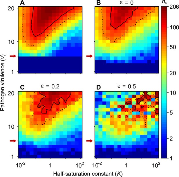
Number of coexisting alleles for eight pathogens as a function of pathogen virulence $v$ and the half-saturation constant $K$ for symmetrically (A) and non-symmetrically placed pathogen vectors (B–D).

Figures are based on a single individual-based simulation per pixel and run for 10⁶ generations, assuring that the equilibrium distribution of alleles is reached. (A) shows results for equally spaced pathogen vectors and isotropic functions $e_{k}$ (Equation A14). It is identical to the bottom right panel in Figure 4 and shown here for comparison. (B–D) show the result for increasing perturbations from symmetry. In (B), pathogen vectors are placed randomly (see Section ‘Random placement of pathogen vectors’ for details) while the functions $e_{k}$ are kept rotationally symmetric. In (C) and (D), additionally to the non-symmetric placement of pathogen vectors, the functions $e_{k}$ are independently perturbed from rotational symmetry (see Appendix ‘Random covariance matrices for the pathogen efficiencies’ for details). In (C) the deviations from rotational symmetry are moderate, while in (D) they are strong. Note that in (B–D) pathogen vectors are no longer at a constant distance 1, but instead have the mean variance calculated from the pathogen optima corresponds to the variance of symmetrically placed pathogens optima with distance 1. Results are reported in terms of the effective number of alleles $n_{e}$ , which discounts for alleles arising from mutation-drift balance (see Appendix ‘Effective number of alleles’). Dashed and solid lines give the contours for $n_{e} = 50$ and $n_{e} = 100$ , respectively. Red arrows indicate $v = 2 \sqrt{8}$ , the minimal value for polymorphism to emerge from branching under full symmetry (Equation A46). Accordingly, simulations in the dark blue area result in a single abundant allele with $n_{e}$ close to one. Other parameters: population size $N = 10^{5}$ , per capita mutation probability $μ = 5 \times 10^{- 7}$ , expected mutational step size $δ = 0.03$ .

Appendix 6—figure 1

Download asset Open asset

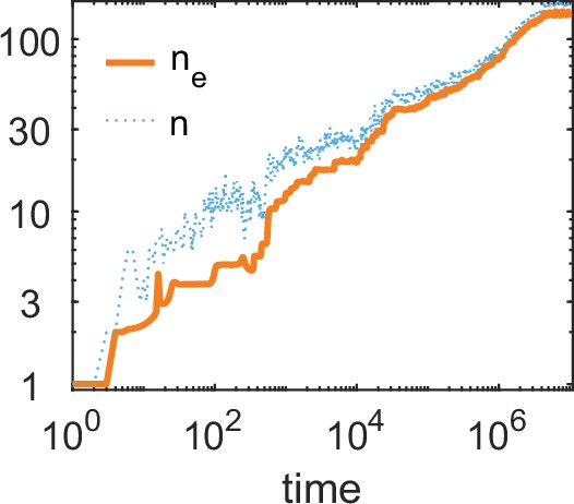
The number of alleles $n$ and the effective number of alleles $n_{e}$ as a function of time (on a log-log plot) for a simulation run of our bit-string model.

Parameters values: $N = 10^{5}$ and $μ = 5 \times 10^{- 6}$ . Other parameters as in Borghans et al., 2004: $v = 7$ , $m = 50$ , $n_{p e p} = 20$ .

Additional files

MDAR checklist: https://cdn.elifesciences.org/articles/94587/elife-94587-mdarchecklist1-v2.pdf
Download elife-94587-mdarchecklist1-v2.pdf

Download links

A two-part list of links to download the article, or parts of the article, in various formats.

Downloads (link to download the article as PDF)

Article PDF

Open citations (links to open the citations from this article in various online reference manager services)

Mendeley

Cite this article (links to download the citations from this article in formats compatible with various reference manager tools)

Mattias Siljestam
Claus Rueffler

(2024)

Heterozygote advantage can explain the extraordinary diversity of immune genes

eLife 13:e94587.

https://doi.org/10.7554/eLife.94587

Sign up for email alerts

Privacy notice